Ultra-short-term PV power prediction using optimal ELM and improved variational mode decomposition

The development of photovoltaic (PV) power forecast technology that is accurate is of utmost importance for ensuring the reliability and cost-effective functioning of the power system. However, meteorological factors make solar energy have strong intermittent and random fluctuation characteristics, which brings challenges to photovoltaic power prediction. This work proposes, a new ultra-short-term PV power prediction technology using an improved sparrow search algorithm (ISSA) to optimize the key parameters of variational mode decomposition (VMD) and extreme learning machine (ELM). ISSA’s global search capability is enhanced by levy flight and logical chaotic mapping to search the optimal number of decomposition and penalty factor of VMD, and VMD adaptively decomposes PV power into sub-sequences with different center frequencies. Then ISSA is used to optimize the initial weight and threshold of ELM to improve the prediction performance of ELM, the optimized ELM predicts each subsequence and reconstructs the prediction results of each component to obtain the final result. Furthermore, isolated forest (IF) and Spearman correlation coefficient (SCC) are respectively used in the data preprocessing stage to eliminate outliers in the original data and determine appropriate input features. The prediction results using the actual data of solar power plants show that the proposed model can effectively mine the key information in the historical data to make more accurate predictions, and has good robustness to various weather conditions.

1 Introduction

Due to the significant increase in global energy demand, traditional energy is facing great challenges such as a lack of resources and environmental pollution (Kumari and Toshniwal, 2021), finding new energy substitutes and improving energy conversion efficiency are the important work of researchers at present (Liu et al., 2021a). Making full use of solar energy is of great significance in reducing fossil energy consumption (Liu et al., 2022). PV power, uses the photovoltaic effect to convert solar energy into electric energy (Liu et al., 2021b), a distributed source of renewable, clean, and flexible energy, is crucial in supplying the world’s rising demand for clean energy (Li et al., 2020). It is imperative to vigorously develop new energy power represented by solar energy and promote the grid connection of a high proportion of renewable energy to build a new power system (Qu et al., 2021). The International Energy Agency estimates that by the end of 2021, there will be 942 GW of cumulative installed PV capacity worldwide, an increase of 22.8% from 2020 (Huang et al., 2022). However, issues including intermittent penetration, voltage spike, reverse power flow, and voltage harmonic distortion brought on by the unpredictability of PV output have gotten worse as the amount of PV in the electrical system has increased (Shivashankar et al., 2016), which greatly affects the stability of power system operation and dispatching capability, making the grid increasingly demanding the PV system’s timely dependability and security (Wang et al., 2022a).

PV power prediction may estimate future output power based on historical data, which is useful for real-time power grid dispatching, minimizing the quality improvement of PV grid connection, and achieving greater economic and social benefits (Ahmed et al., 2020). As a result, several academics started concentrating on ways to increase the precision of PV output prediction.

Four categories of PV power forecasting techniques can be established based on various prediction time scales: short-, medium-, long-, and ultra-short-term (UST) (Voyant et al., 2017). The UST forecast usually considers PV output in the next 1 min to 1 h, which is used for the power smoothing process, PV storage control, and real-time power dispatching monitoring (Rodríguez et al., 2022). The short-term forecast’s time frame is several hours, and prediction results can be used in short-term economic load dispatching and power system operation (Das et al., 2018). For medium- and long-term predictions, the days or weeks are often the time scale employed; these forecasting technologies are mostly used for dispatching and power production planning of PV power plants (Akhter et al., 2019). Because solar power has a high degree of randomness, it is difficult for existing methods to capture the rapid fluctuations of PV power in a short time, especially in unconventional weather conditions (Wang et al., 2015). Therefore, the focus of current research is on short- and ultra-short-term prediction (Li et al., 2021).

At present, there are two main types of solar power forecast technology: physical models and data-driven models (Schinke-Nendza et al., 2021). The former needs to use the detailed geographic information and specific equipment parameters of the PV power station, combine the numerical weather prediction (NWP), and calculate the prediction results according to the formula. The modeling process is relatively complex and is greatly affected by the model parameters (Wang et al., 2019). The data-driven methods use an intelligent algorithm to study the function mapping between the input data and the solar power, which is characterized by high prediction accuracy and strong robustness (Sohani et al., 2022). Some researchers use data-driven models to enhance the precision of solar energy prediction in light of the recent rapid growth of data mining and artificial intelligence technology (Yagli et al., 2019). Among them, artificial neural networks (ANN) related technologies are popular because of their strong non-linear fitting ability (Lu et al., 2021).

The research on improving the prediction accuracy of solar power mainly focuses on two aspects, one is to establish a more reliable and accurate prediction model. For example, in Zhang et al. (2019), spatial similarity and temporal correlation were used to analyze similar time-varying patterns that may occur in PV systems at different locations, and a Bayesian neural network is used for solar power prediction, which has better application performance than many baseline methods. In Ko et al. (2022), by adding hidden layers, the convolutional neural network (CNN) model’s capacity for feature extraction was enhanced, but it also brought huge computational challenges while improving the prediction accuracy. In Agga et al. (2021), to extract PV features, CNN and long short-term memory (LSTM) network are combined with higher accuracy when compared to a solo CNN or LSTM.

Additionally, by applying the meta-heuristic algorithm to optimize the neural network’s parameters, the model’s ability to predict outcomes can be enhanced. Common meta-heuristic algorithms include particle swarm optimization (PSO), gray wolf optimization (GWO), whale optimization algorithm (WOA), etc. In Tu et al. (2022), regression neural network (GRNN) accuracy is increased via GWO optimization. In Xu et al. (2022), WOA was used to improve the super parameters of bidirectional LSTM (BILSTM). Finally, the prediction effect of BILSTM was significantly improved after WOA optimization.

Compared with traditional neural networks, rapid learning and a simple model structure are advantages of ELM, but the initial parameters have a significant impact on the prediction outcomes (Du et al., 2022). In An et al. (2021), Zhang et al. (2022), the performance of the ELM prediction is optimized using sparrow search algorithm (SSA) to lower the uncertainty caused by the input weights and thresholds. The findings demonstrate that SSA outperforms the traditional PSO meta-heuristic technique in terms of optimization impact, but SSA is still prone to settle for the local optimal solution during the search phase. In Jia et al. (2021), the search step of SSA is optimized by using Levy flight, but the initial position distribution of SSA population still limits its global search ability.

Another aspect of improving prediction performance is to use better methods to preprocess the original data. Because solar power is highly non-linear and non-stationary, when the original data is employed as the model input features, it is difficult for the forecasting model to extract important information from the historical data, especially in periods with large meteorological fluctuations. For this reason, Some researchers develop numerous models to determine the specific changing features of each subsequence after breaking down the original PV sequence using frequency domain decomposition technology (Sulandari et al., 2020). Many well-liked signal decomposition techniques were reported, such as wavelet decomposition (WD), empirical mode decomposition (EMD), ensemble empirical mode decomposition (EEMD) (Wang et al., 2022b), etc.

In Wang D. et al. (2022), EMD was employed to lessen the series’ non-stationarity. However, there was mode aliasing in the decomposition process of EMD, which would interfere with the final prediction results. In Zhu A. et al. (2022), wind power is predicted by complementary ensemble empirical mode decomposition (CEEMD), WOA, and Elman neural networks, which reduces the phenomenon of mode aliasing in the decomposition process of EMD and EEMD, and further improves the prediction performance. In Lu et al. (2022), VMD and weighted replacement entropy (WPE) were used to extract key factors of historical data as model inputs, and good prediction results were achieved on multiple wind farm datasets.

VMD can effectively avoid mode aliasing and has good anti-interference performance for time series with large noise, the effect of processing non-linear signals has been proven to be superior to EMD and its improved methods (Xie et al., 2018). But VMD requires manually preset penalty factor $\alpha$ and the number of decomposition $K$, which may affect the prediction accuracy (Zhang et al., 2020).

Based on the above analysis, this study improved the traditional SSA, optimized the parameters of VMD and ELM using ISSA, and built a new hybrid PV output forecasting model. The following summarizes this paper’s primary contributions.

1. Levy flight optimizes the step size of each SSA search to enhance the ability of SSA to jump out of local optimum. In addition, Logistic chaotic mapping makes the initial position distribution of sparrow more uniform, it avoids that some areas cannot be searched due to the random setting of the initial position. The combination of these two methods can simultaneously improve the individual search distance and the overall search range, thus improving the global search ability of SSA.

2. ISSA decreases the signal loss in the decomposition process, making subsequence prediction easier by optimizing the VMD’s decomposition number and penalty factor while avoiding the randomness of the experience setting.

3. In order to further enhance the ELM’s predictive performance, ISSA is also employed to tune the initial weight and threshold.

4. SCC is employed to identify the meteorological characteristics that have a strong correlation with solar power, and in order to prevent irrelevant characteristics and aberrant data from interfering with the prediction results, the IF algorithm is used to identify outliers.

5. A hybrid forecasting technique is proposed. The data from the DKASC PV experiment center in Australia is used for prediction, and the suggested model’s excellent performance is demonstrated by comparing its prediction outcomes to those of existing models under various weather situations.

The rest components of the work were organized as follows: Section 2 introduces the basic methods used in this study, including VMD, ELM, SSA, and the proposed improvement strategy for SSA. Section 3 shows ISSA’s optimization process for VMD and ELM, as well as the basic framework for the model. Section 4 displays the test’s outcomes and analysis.

2 Materials and methods

2.1 Variational modal decomposition

VMD was proposed in 2013 as a non-recursive signal decomposition technology (Dragomiretskiy and Zosso, 2013), which decomposes the non-stationary signal to intrinsic mode functions (IMF) by iteratively finding the variational model’s optimal solution. Although VMD suppresses the end effect and modal aliasing of traditional frequency domain decomposition technology, it needs to be set in advance $\left(K,\alpha \right)$ Parameters. The decomposition procedure of VMD is presented below:

1. Set the decomposition $K$ number, take the original signal then break it down into IMF sequences. In the decomposition process, the goal function is the minimum total of the frequency bandwidths of each IMF, and the requirement is that the original signal is equal to the total of all IMF sequences.

$\left\{\begin{array}{l}\underset{\left(u_k,w_k\right)}{\mathit{min}}\left\{{\displaystyle \sum _{k=1}^K}{\partial }_t\left[\left(\delta \left(t\right)+\frac{j}{\pi t}\right)*u_k\left(t\right)\right]e^{-j{\omega }_k{t}_2^2}\right\}\\ s.t.{\displaystyle \sum _{k=1}^K}{u}_k\left(t\right)=f\left(t\right)\end{array}\right.(1)$

Where $\delta \left(t\right)$ obeys Dirac distribution; $u_k\left(t\right)$ is the corresponding IMF after decomposition; $w_k$ is the center frequency of $u_k\left(t\right)$; $*$ represents a convolution operation.

2. Set penalty factor $\alpha$, using Lagrange multipliers $\lambda$ transforming the above constrained variational problem into an unconstrained problem.

$L\left(u_k,{\omega }_k,\lambda \right)=\alpha {\displaystyle \sum _{k=1}^k}\parallel {{\partial }_t\left\{\left[\delta \left(t\right)+\frac{j}{\pi t}\right]*u_k\left(t\right)\right\}\cdot e^{-j{\omega }_{k}t}\parallel }_2^2+{\parallel f\left(t\right)-{\displaystyle \sum _{k=1}^k}{u}_k\left(t\right)\parallel }_2^2+⟨\lambda \left(t\right),f\left(t\right)-{\displaystyle \sum _{k=1}^k}{u}_k\left(t\right)⟩(2)$

3. Solve the unconstrained problem in Equation 2 using the multiplier alternating direction method (ADMM), iteratively update $u_k$ and ${\omega }_k$:

${\widehat{u}}_k^{n+1}\left(\omega \right)=\frac{\widehat{f}\left(\omega \right)-{{\displaystyle \sum }}_{i\ne k}{\widehat{u}}_i\left(\omega \right)+\frac{\widehat{\lambda }\left(\omega \right)}{2}}{1+2\alpha {\left(\omega -{\omega }_k\right)}^2}(3)$

${\omega }_k^{n+1}=\frac{{\int }_0^{\infty }\omega {\left|{\widehat{u}}_k^{n+1}\left(\omega \right)\right|}^{2}d\omega }{{\int }_0^{\infty }{\left|{\widehat{u}}_k^{n+1}\left(\omega \right)\right|}^{2}d\omega }(4)$

Where ${\widehat{u}}_i\left(\omega \right)$, $\widehat{f}\left(\omega \right)$, $\widehat{\lambda }\left(\omega \right)$ are the Fourier transforms of the points $u_i\left(t\right)$, $f\left(t\right)$, $\lambda \left(t\right)$, respectively; n denotes the number of iterations.

2.2 Extreme learning machine

Different from traditional SLFN (Huang et al., 2006), in ELM, the connection weight $w$ and threshold $b$ are randomly generated (Figure 1). Using the generalized inverse matrix and the least squares approach, the $\beta$ weight of the output layer is determined. As a result, ELM offers the advantages of requiring little in the way of training parameters and learning quickly (Hu et al., 2022).

FIGURE 1

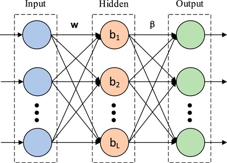
FIGURE 1. Diagram of the ELM network’s structure.

In Figure 1, suppose that the input $\left\{x_i\right\}$ is composed of $m$ samples and $n$ features, and L is the ELM’s hidden layer node count. The expression of ELM output $F\left(x_i\right)$ is:

$F\left(x_i\right)={\displaystyle \sum _{i=1}^L}{\beta }_i·g\left(w_i{x}_i+b_i\right)(5)$

Where $w_i$ is the input weight; $b_i$ is hidden layer threshold; ${\beta }_i$ is output weight; $g$ is activation function.

When using matrix $H$ to represent hidden layer output, then the output matrix $F$ of ELM can be expressed as:

$F=\beta H(6)$

ELM solves the output layer weight $\beta$ by minimizing the error:

${\mathit{min}\parallel F-Y\parallel }^2(7)$

$\beta =Y{H}^{+}(8)$

$H^{+}$ represents the generalized inverse matrix of $H$.

2.3 Sparrow search algorithm

The technique was introduced to address the issue of global optimization by imitating the feeding habits of a population of sparrows (Xue and Shen, 2020). Compared with the traditional meta-heuristic learning algorithm, SSA has certain advantages in convergence speed and stability (Ma et al., 2022). SSA assumes that there are three kinds of sparrows: discoverers, followers, and guards, each sparrow’s position correspond to a solution. The fitness function is used by SSA during the optimization phase to determine how far away the food is from the present location of the sparrow. The optimal posture is considered to be the one with the greatest food or the position with the best fitness.

The discoverer is in charge of locating food and giving followers instructions on what to do, and it is updated below:

$S_{i,j}^{t+1}=\left\{\begin{array}{ll}{S}_{i,j}^t\cdot \exp \left(\frac{-i}{\lambda \cdot n}\right),& E<ST\\ S_{i,j}^t+Q\cdot L,& E>ST\end{array}\right.(9)$

Where $S_{i,j}^t$ is the $i$ th discoverer’s location at the $j$ dimension in the $t$ iteration; $\lambda \in \left[\mathrm{0,1}\right]$ is a random number; $Q$ is a random variable with a normal distribution; $L$ is the $1\times d$ identity matrix; $E\in$ [0,1] is a warning value; $ST\in \left[\mathrm{0.5,1}\right]$ is a safety value.

The expression of followers’ location is as follows:

$S_{i,j}^{t+1}=\left\{\begin{array}{ll}{S}_b^{t+1}+\left|S_{i,j}^t-S_b^{t+1}\right|\cdot A^{+}\cdot L,& i\le \frac{n}{2}\\ Q\cdot \exp \left(\frac{S_w^t-S_{i,j}^t}{i^2}\right),& i>\frac{n}{2}\end{array}\right.(10)$

$A^{+}=A^T{\left(A{A}^T\right)}^{-1}(11)$

Where $S_{i,j}^{t+1}$ is the global optimal position among discoverers in $t+1$ iterations; $S_w^t$ represents the global worst position at iteration $t$; A is $1\times d$ matrix with elements of 1 or - 1; when $i>\frac{n}{2}$, the fitness of the population is low, and the search scope needs to be expanded; when $i\le \frac{n}{2}$, the sparrow population can feed randomly at position $S_b^{t+1}$.

The guards make up 10%–20% of the total, and their location is updated as follows:

$S_{i,j}^{t+1}=\left\{\begin{array}{ll}{S}_b^t+\omega \left|S_{i,j}^t-S_b^t\right|,& F_i>F_b\\ S_{i,j}^t+P\cdot \left(\frac{S_{i,j}^t-S_w^t}{F_i-F_w+\epsilon }\right),& F_i=F_b\end{array}\right.(12)$

Where $S_b^t$ represents the global best position in iteration $t$; $\omega$ is the step control parameter, $\omega \sim N\left(\mathrm{0,1}\right)$; $P\in \left[-\mathrm{1,1}\right]$ controls the direction and step size of sparrow updates using a random value; $\epsilon$ is a necessary constant to prevent the denominator from becoming zero; $F_i$, $F_b$, and $F_w$, respectively, signify the fitness values of the current sparrow, the best bird, and the poorest sparrow.

2.4 Improved sparrow search algorithm

Traditional SSA first randomly gives each sparrow initial position information, which is taken as a solution of the parameters. Then, according to the SSA location update method and fitness function, search and iterate continuously until the global optimal solution is determined. Since the initial population position is a randomly assigned variable in the search interval, if the initial position is unevenly distributed, it will lead to low population diversity and affect the final convergence accuracy. In addition, because SSA is affected by the position update step size in each iteration, it is difficult to leave the locally optimum option. Therefore, to improve SSA’s ability to conduct global searches, this study uses the Levy flight and Logistic chaotic mapping to improve SSA.

2.4.1 Levy flight strategy

Levy flight strategy can generate random step size, so as to strengthen the interaction of population information, expand the search scope, and increase the capacity to break out of the local optimal state (Iacca et al., 2021). The formula of Levy flight is as follows:

$s=\frac{\mu }{{\left|v\right|}^{1/\beta }}(13)$

$\left\{\begin{array}{c}v\sim N\left(0,{\sigma }_v^2\right)\\ \mu \sim N\left(0,{\sigma }_{\mu }^2\right)\end{array}\right.(14)$

$\left\{\begin{array}{l}{\sigma }_v=1\\ {\sigma }_{\mu }={\left\{\frac{\mathrm{\Gamma }\left(1+\beta \right)·\sin \left(\pi \beta /2\right)}{\beta ·\mathrm{\Gamma }\left[\frac{1+\beta }{2}\right]·2^{\left(\beta -1\right)/2}}\right\}}^{1/\beta }\end{array}\right.(15)$

Where $s$ is the random step size; $\beta$ Is the control coefficient between [0,2].

The Levy flight method is applied in this study to update the sparrow’s position. The random step $s$ obtained by Levy flight is used to replace the original random number $Q$ in the formula (9), (10) of SSA. After improvement, the location update formula (9) of the discoverer is changed into formula (16):

$S_{i,j}^{t+1}=\left\{\begin{array}{ll}{S}_{i,j}^t\cdot \exp \left(\frac{-i}{\lambda \cdot n}\right),& E<ST\\ S_{i,j}^t+s\cdot L,& E>ST\end{array}\right.(16)$

The position of the follower is updated by Formula (10), which is transformed into Formula (17) after improvement:

$S_{i,j}^{t+1}=\left\{\begin{array}{ll}{S}_b^{t+1}+\left|S_{i,j}^t-S_b^{t+1}\right|\cdot A^{+}\cdot L,& i\le \frac{n}{2}\\ s\cdot \exp \left(\frac{S_w^t-S_{i,j}^t}{i^2}\right),& i>\frac{n}{2}\end{array}\right.(17)$

2.4.2 Logistic chaotic mapping

Logistic chaotic mapping uses a simple random sequence of the deterministic system to generate the chaotic sequence, which has boundedness, randomness, and ergodicity. This method can traverse all states within a certain range, thus increasing the diversity of the population (Hu et al., 2020), avoid that some areas cannot be searched. The expression equation is:

$Z_n=\mu ·Z_{n-1}·\left(1-Z_{n-1}\right),n\in N^{*}(18)$

Where $Z_n$ obeys uniform distribution in [0,1]; $\mu$ Is the control parameter in [0,4].

The control parameter $\mu$ in this study is set to 4 so that the distribution is completely chaotic. The initial position is set according to the Logistic chaotic mapping, and the expression formula is as follows:

$x_n=b_l+\left(b_u-b_l\right)·Z_n(19)$

Where $b_u$, $b_l$ are the boundaries of the search range.

3 Construction of ISSA-VMD-ELM model

3.1 VMD optimized by ISSA (ISSA-VMD)

The initial parameter $\left(K,\alpha \right)$ of VMD will affect the decomposition effect of PV power, thus affecting the prediction performance. Therefore, ISSA is used to optimize it to reduce the learning cost of the forecasting model for each IMF after decomposition.

Envelope entropy can measure the fluctuation and complexity of time series data. Entropy decreases when the time series’ apparent periodicity increases; on the other hand, entropy increases as data complexity and volatility increase (Gao et al., 2022). In the decomposition process, Envelope entropy is used as an indicator to measure the decomposition effect of VMD. The smaller the envelope entropy after decomposition, the better the decomposition effect. Envelope entropy is calculated as follows:

$\left\{\begin{array}{c}{E}_p=-{\displaystyle \sum _{j=1}^N}{p}_{i,j}\cdot \mathit{lg}\left(p_{i,j}\right)\\ p_{i,j}=a_i\left(j\right)/{\displaystyle \sum _{j=1}^N}{a}_i\left(j\right)\end{array}\right.(20)$

Where $p_{i,j}$ represents the normalized form of $a_i\left(j\right)$; $a_i\left(j\right)$ represents the envelope signal of ${IMF}_i$ after the Hilbert transform.

In the process of ISSA optimizing VMD, the position of each sparrow represents a set of parameters $\left(K,\alpha \right)$, VMD decomposition of PV power is performed with this parameter, and $E_p$ is calculated as fitness. The population position is optimized in the direction of $E_p$ minimum. When the iteration termination condition is reached, the parameter $\left(K,\alpha \right)$ corresponding to the least $E_p$ is regarded as the result. Figure 2 illustrates the optimization procedure of ISSA-VMD. The following is the precise implementation strategy:

1. Initialize the sparrow population parameters.

2. Initialize the position of each sparrow according to Equation 19.

3. Based on the position parameters $\left(K,\alpha \right)$ of each sparrow, the VMD is utilized to decompose the solar power, then the $E_p$ value is calculated according to Equation 20 as the fitness of the sparrow at this location.

4. Update the discoverer’s location in accordance with Equation 16, the location of the follower according to Equation 17, and the location of the guard according to Equation 12 to make the sparrow population close to the minimum fitness value.

5. Once the max iterations have been achieved, the sparrow location with the lowest fitness should be noted and utilized as the ideal VMD parameter, otherwise repeat steps 3 and 4.

FIGURE 2

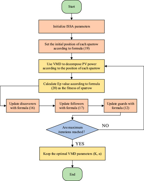
FIGURE 2. Flow chart of ISSA-VMD.

3.2 ELM optimized by ISSA (ISSA-ELM)

The ELM’s threshold $b$ and input weight $w$ are created at random. These randomly generated initial values will directly affect the final prediction effect, so this study uses ISSA to optimize the parameter of ELM, in the optimization process, the position of each sparrow represents a set of $\left(w,b\right)$ parameters of ELM, the fitness metric utilized is mean square error (MSE):

$e_{MSE}=\frac{1}{N}{\displaystyle \sum _{t=1}^N}{\left(P_t-P_t^{\prime }\right)}^2(21)$

$P_t$ represents the real value; $P_t^{\prime }$ represents predicted value.

The exact processes for ISSA-ELM are as follows. Figure 3 illustrates the optimization procedure of ISSA-ELM.

1. Set the settings for the sparrow population.

2. Give each sparrow a random initial position according to Formula (19).

3. Based on the position parameters $\left(w,b\right)$ of each sparrow, ELM is used for PV power prediction. Calculate the MSE of prediction results according to Equation 21 and take it as the fitness value at this location.

4. Update the discoverer’s location in accordance with equation (16), the location of the follower according to equation (17), and the location of the guard according to equation (12) to make the sparrow population close to the minimum fitness value.

5. Steps 3 and 4 should be repeated until the max iterations are reached, and retain the sparrow position corresponding to the minimum MSE value as the input weight and threshold $\left(w,b\right)$ of ELM.

FIGURE 3

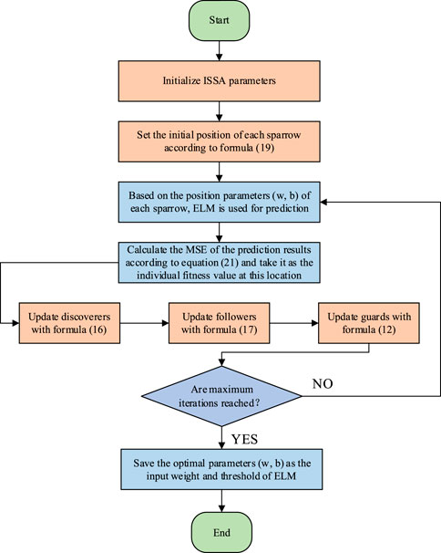
FIGURE 3. ISSA-ELM flow chart.

3.3 Error evaluation metrics

MAPE, RMSE, and determination coefficient ($R^2$) are selected as the model evaluation indicators. MAPE, RMSE, and $R^2$ are calculated as follows:

$e_{MAPE}=\frac{1}{N}{\sum }_{t=1}^N\left(\left|\frac{P_t^{\prime }-P_t}{P_t}\times 100\%\right|\right)(22)$

$e_{RMSE}=\sqrt{\frac{1}{N}{\sum }_{t=1}^N{\left(P_t-P_t^{\prime }\right)}^2}(23)$

$R^2=1-\frac{{\displaystyle \sum _{t=1}^N}{\left(P_t^{\prime }-P_t\right)}^2}{{\sum }_{t=1}^N{\left(\overline{P_t}-P_t\right)}^2}(24)$

$P_t$ represents real value; $P_t^{\prime }$ represents predicted value; $\overline{P_t}$ represents sample mean value.

3.4 Framework of the proposed hybrid model

The IF algorithm is used in this study in addition to the aforementioned optimization techniques to remove outliers from the original data. Considering that PV output is affected by different meteorological features to a different extent, SCC is employed to identify important climatic traits that are strongly connected with PV power. At the same time, autocorrelation analysis (ACF) is used to choose the appropriate length of the input of the prediction model. These techniques can lessen the prediction model’s training requirements as well as the impact of data impurities and redundancy on prediction accuracy. Figure 4 displays the suggested model’s prediction procedure, and these are the precise steps:.

1. The original data’s outliers are removed using the IF method, then the missing values are interpolated and filled, and the training set and test set are divided.

2. Analysis of meteorological characteristics using SCC. Identify a few meteorological variables that have a strong relationship to PV power.

3. The VMD parameter $\left(K,\alpha \right)$ are optimized by ISSA to decompose the PV power.

4. For each IMF after decomposition, train the corresponding ISSA-ELM model to predict PV power. During training, IMF and meteorological data before the prediction are utilized as the model input and the length is determined using ACF, and the actual PV power at the prediction point is used as the prediction target.

5. To get the final prediction results, all subsequences’ predicted values are reassembled.

6. Analyze forecast results using error evaluation indicators.

FIGURE 4

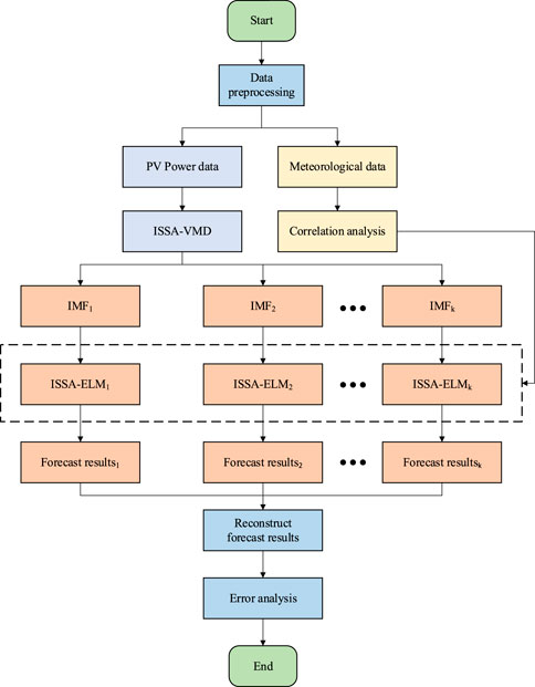
FIGURE 4. The forecasting model’s flowchart.

4 Case study

4.1 Source of data

The information comes from the Desert Knowledge Australian Solar Center’s Alice (DKASC) Springs PV power facility (DKASC, 2008), which provides multiple PV array data, as shown in Figure 5A. In addition, DKASC also provided meteorological data of the region, including global horizontal radiation (GHR), diffuse horizontal radiation (DHR), etc. The historical data of the 16A_BP_Solar PV array was used for test analysis, the resolution of data is 5 min 80% of them are training sets and 20% are test sets. The actual structure of this PV array is shown in Figure 5B, and Table 1 displays the fundamental parameter information.

FIGURE 5

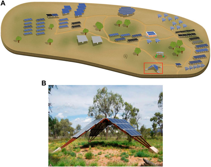
FIGURE 5. Schematic diagram of (A) DKASC Alice Springs PV power station, (B) 16A_BP_Solar PV array (DKASC, 2008).

TABLE 1

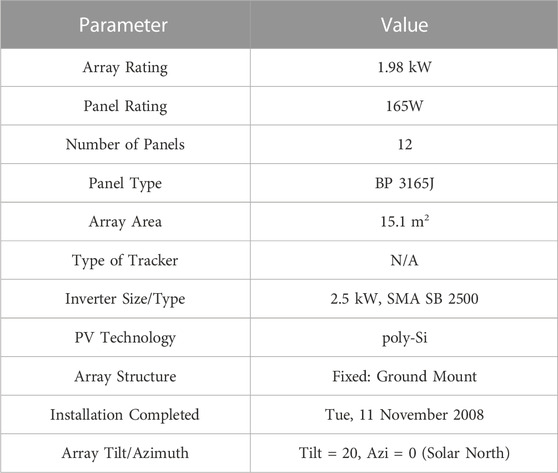
TABLE 1. Basic parameters of 16A_BP_Solar PV array.

4.2 Data preprocessing

4.2.1 Data cleaning

The period of data is selected from 7:30 a.m. to 18:00 p.m. (126 nodes). Due to the failure of recording equipment, damage to PV modules, interference in information transmission, and other reasons, there are some abnormal values and missing values in the original data. To prevent this data’s negative influence on the prediction, the IF algorithm is utilized to identify outliers. IF algorithm is an unsupervised learning algorithm that identifies exceptions by isolating them from data (Hanifi et al., 2022). Based on the characteristic that PV power increases linearly with GHR, GHR and PV power are used as the IF algorithm’s input features (Figure 6).

FIGURE 6

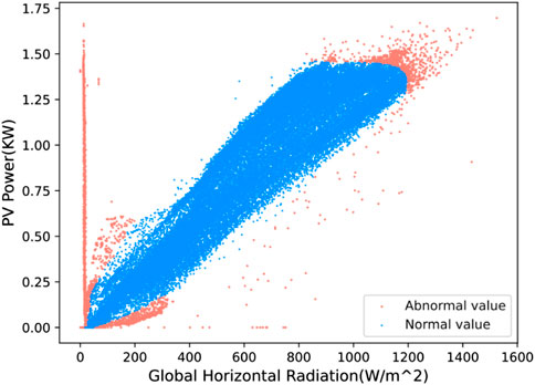
FIGURE 6. Abnormal value detection results of IF algorithm.

Figure 6 shows that the IF algorithm effectively identifies abnormal values in PV data, mainly including: (1) The point without irradiance but with PV power output. (2) The point with irradiance but no PV power output. (3) Outliers that differ from most data distributions. This research uses the mean insertion technique to fill in missing data values. Figure 7A depicts a portion of the raw data prior to processing, and Figure 7B depicts a portion of data after processing.

FIGURE 7

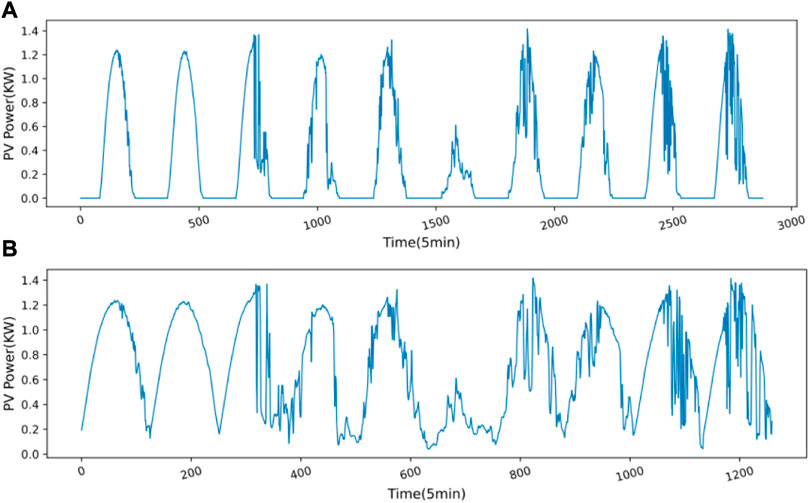
FIGURE 7. PV power data (A) before processing, (B) after processing.

4.2.2 Selection and processing of input features

PV power is influenced by a variety of weather characteristics. However, different meteorological features have different effects on PV power, and excessive input features will reduce the sensitivity of the model to important features (Zhu Y. et al., 2022).

In this study, SCC is used to identify the input meteorological characteristics and assure the ability to extract important meteorological features. Below is the calculation formula of SCC (Figure 8).

$\mathrm{S}\mathrm{C}\mathrm{C}=\frac{{\displaystyle \sum }_i\left(x_i-\overline{x}\right)\left(y_i-\overline{y}\right)}{\sqrt{{\displaystyle \sum }_i{\left(x_i-\overline{x}\right)}^2{\displaystyle \sum }_i{\left(y_i-\overline{y}\right)}^2}}(25)$

Where $x_i$ and $y_i$ represent meteorological characteristics and PV power respectively; $\overline{x}$ and $\overline{y}$ represents the average value of $x_i$ and $y_i$ respectively.

FIGURE 8

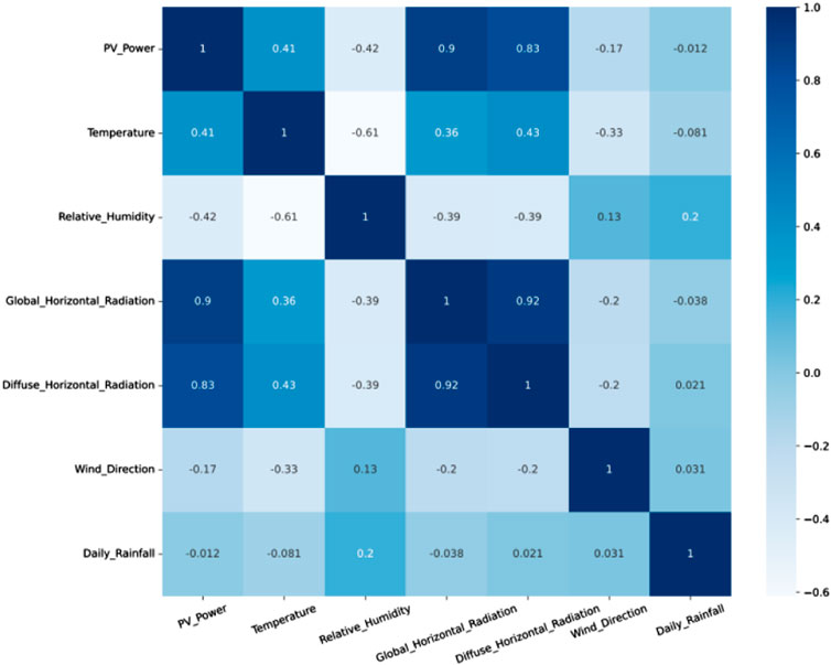
FIGURE 8. Results of SCC correlation analysis.

Figure 8 shows that GHR and DHR have the highest correlation with PV power, 0.9 and 0.83 respectively. The SCC of temperature and PV power is 0.41, which is of medium correlation. Therefore, the meteorological characteristics input into the prediction model is selected as GHR, DHR, and temperature. The correlation between other meteorological characteristics and PV power is too low, which is regarded as redundant characteristics and is not used as model input. To sum up, the model input characteristics can be determined (Table 2).

TABLE 2

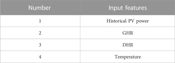
TABLE 2. Proposed model’s input features.

The length of the input features is determined by ACF, which is utilized to measure the impact of historical data (Figure 9).

FIGURE 9

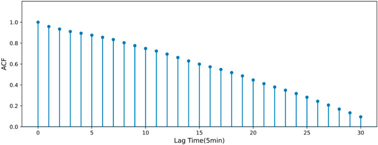
FIGURE 9. Autocorrelation analysis results of PV power based on ACF.

In order to avoid the increase of model complexity caused by too long an input sequence and the interference of data at early time points to the prediction results, this paper selects 15 nodes with strong PV power correlation (≥0.6) at the current time point as the input.

Finally, to avoid having differing feature dimensions affect the model, the input features are standardized with the Min-Max approach. Below is the equation:

$x_{norm}=\frac{x-x_{\mathit{min}}}{x_{\mathit{max}}-x_{\mathit{min}}}(26)$

Where $x_{norm}$ is the normalized value of $x$; $x_{\mathit{max}}$ and $x_{\mathit{min}}$ are the maximum and minimum values in the sequence respectively.

4.3 Analysis of Experimental results

The test was conducted in the Anaconda environment of the Windows 10 operating system, the Python version is 3.9, and basic hardware includes AMD-5800X CPU and NVIDIA-3070TI GPU (Table 3).

TABLE 3

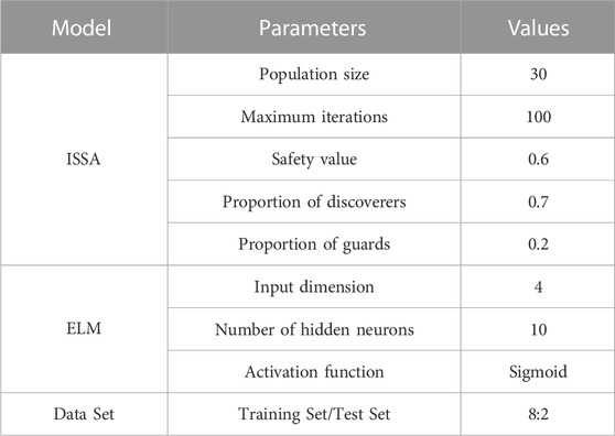
TABLE 3. Settings for the suggested model’s parameters.

4.3.1 Performance analysis of ISSA

To reflect the optimization performance of ISSA, this section analyzes the decomposition effects of ISSA-VMD, SSA-VMD, and VMD (Figure 10).

FIGURE 10

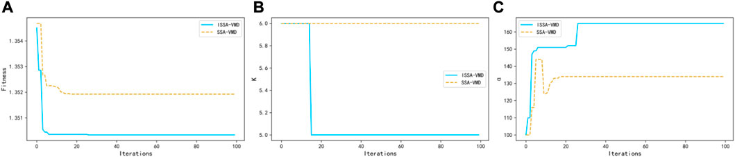
FIGURE 10. Comparison of VMD parameter optimization effects: (A) is the result of fitness optimization, (B) is the optimization result of decomposition number $K$, and (C) is the optimization result of penalty factor $\alpha$.

Figure 10 illustrates that ISSA has a better optimization effect on VMD than traditional SSA algorithm, and can quickly obtain smaller fitness values. The optimization effect of traditional SSA on $K$ value is not obvious, and entering the local optimum solution is simple. The VMD decomposition effect using ISSA, SSA optimization algorithm, and empirical parameter settings is shown in Table 4. After ISSA optimization, the $K$ and $\alpha$ of VMD are finally determined as (5, 165).

TABLE 4

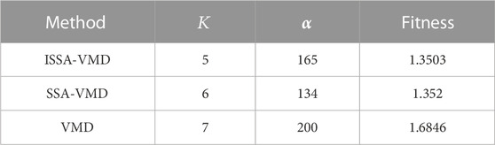
TABLE 4. Comparison of effects of different decomposition methods.

The decomposition results of ISSA-VMD on PV power data are illustrated in Figure 11. It shows how ISSA-VMD breaks down the original PV power into five IMFs. The center frequencies of these 5 IMFs are different, which can be clearly distinguished, indicating that there is no mode aliasing among the IMF after ISSA-VMD decomposition.

FIGURE 11

FIGURE 11. Decomposition results of ISSA-VMD: (A) shows each subsequence after decomposition, (B) represents center frequency of each subsequence, and (C) represents spectrum of each subsequence.

In order to evaluate effects of various decomposition techniques on prediction outcomes, three different decomposition methods: ISSA-VMD, SSA-VMD, and VMD, are used in combination with the proposed ISSA-ELM model for prediction comparison. Due to the different fluctuations of PV power under different weather conditions, in order to reduce the impact of weather on the prediction results, the paper forecasts the three different weather conditions (Ma et al., 2022). Figure 12, Figure 13, and Figure 14 demonstrate, respectively, the forecast results and error distribution based on various decomposition techniques for sunny, cloudy, and rainy days. In each weather, three evaluation indicators: RMSE, MAPE, and $R^2$ are used to analyze the prediction results, which are shown in Figure 15.

FIGURE 12

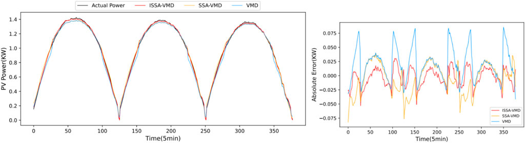
FIGURE 12. Prediction outcomes and error distribution on bright days using various decomposition techniques.

FIGURE 13

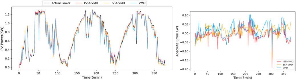
FIGURE 13. Prediction outcomes and error distribution using different decomposition methods on cloudy days.

FIGURE 14

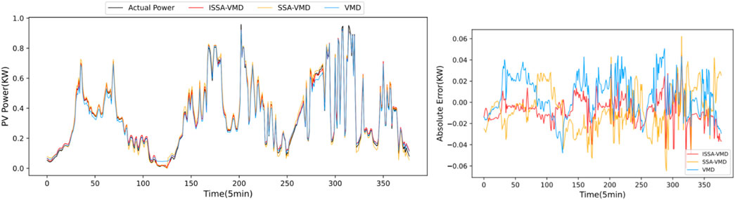
FIGURE 14. Prediction outcomes and error distribution using different decomposition methods on rainy days.

FIGURE 15

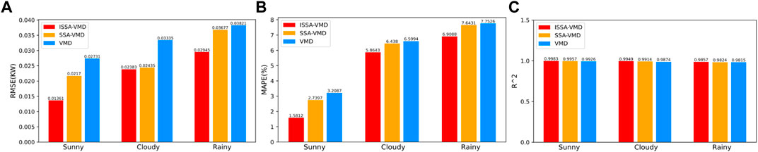
FIGURE 15. The evaluation results in three weather conditions by (A) RMSE, (B) MAPE, (C) $R^2$.

Figures 12–14 demonstrates that the decomposition effect of VMD will impact prediction accuracy. In different weather conditions, the results that may be readily predicted using VMD decomposition differ significantly from the real PV power, and the error fluctuates greatly. Compared with SSA-VMD and VMD, the prediction result using the ISSA-VMD decomposition method has the highest fitting degree with the actual solar power curve, the prediction error has the smallest range of change with time, the most stable fluctuation, and the overall error distribution is the most uniform.

The comparison in Figure 15 shows that ISSA-VMD had the highest performance, and the largest $R^2$ in three weather conditions. Even on rainy days with large weather fluctuations, the RMSE, MAPE, and $R^2$ of the model after ISSA-VMD decomposition are 0.02945 kW, 6.9088%, and 0.9857 respectively, which still maintain good prediction accuracy. The above analysis shows that the improvement of SSA is effective. ISSA strengthens the decomposition effect of VMD, makes the information in the decomposed data easier to be learned by the prediction model, and improves the prediction performance.

4.3.2 Performance analysis of different models

In this section, 5 prediction models: SSA-ELM, ELM, BP, SVM, and proposed ISSA-ELM, are used for PV prediction, and then different models’ prediction effects are evaluated. To make sure the comparison is fair, the decomposition method used are all ISSA-VMD. The prediction results in three typical weather conditions of different models are shown in Figure 16. In addition, to further compare the model’s prediction performance, the prediction results are analyzed with RMSE, MAPE, and $R^2$ in Table 5.

FIGURE 16

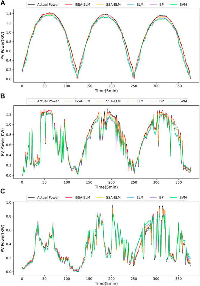
FIGURE 16. Predictions outcomes on (A) sunny days, (B) cloudy days, (C) rainy days.

TABLE 5

TABLE 5. Evaluation indexes of different models in three kinds of weather.

By observing the prediction curves of different models in Figure 16 we found that the forecast accuracy of the ISSA-ELM model proposed is the best, and the prediction results in the three weather conditions are most close to the actual PV power. Not only on sunny days but also in other weather conditions, the output curve of ISSA-ELM is quite close to the real power, which demonstrates the great resilience of the novel model to weather disruptions.

Furthermore, all the indicators of ISSA-ELM in the three kinds of weather are better than other models. Compared with evaluation outcomes of ISSA-ELM, SSA-ELM, and ELM, the optimization algorithm has brought significant performance improvement to the traditional ELM prediction method. On different weather conditions, the RMSE of ISSA-ELM relative to SSA-ELM decreased by 47.25% (sunny), 20.59% (cloudy), and 24.41%(rainy) respectively, and MAPE decreased by 29.3% (sunny), 8.91% (cloudy), and 10.88% (rainy) respectively, $R^2$ is also improved significantly. The preceding analysis demonstrates that the ISSA optimizes ELM more effectively. Compared with the traditional SSA-ELM model, the proposed ISSA-ELM model has better prediction performance under various weather conditions, and has certain robustness to weather fluctuations.

To illustrate the improvement of ISSA and VMD on ELM prediction performance, Figure 17 shows the prediction results of different methods for five consecutive days, and gives the average value of each evaluation index for the five consecutive days in Table 6. Combining Figure 17 and Table 6, it can be found that the prediction result of directly using ELM is not ideal, and ISSA can slightly improve the prediction accuracy of ELM. After using VMD, the prediction results have been greatly improved. Using ISSA to enhance both ELM and VMD at the same time has the best prediction effect and the highest fitting degree with the original PV power.

FIGURE 17

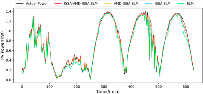
FIGURE 17. Forecast results of different models for 5 consecutive days.

TABLE 6

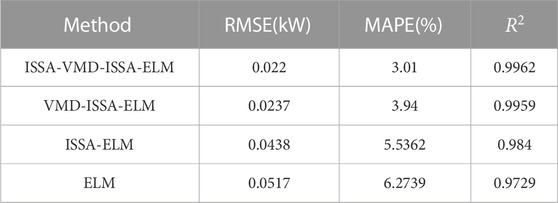
TABLE 6. Evaluation indexes of different models in three kinds of weather.

5 Results

For the power system to operate safely, an accurate PV power forecast is a need. The accuracy of the PV power forecast might be increased by using a hybrid model based on ISSA, VMD, and ELM, according to this research. The outcomes of our study indicate.

1. Our IF algorithm can reasonably eliminate outliers in the PV data set, and SCC can find the features that have the highest correlation with PV power generation, laying a foundation for the training of the prediction model.

2. Compared with traditional SSA, the proposed ISSA has better global search capability.

3. The VMD optimized by ISSA has a better ability to decompose non-linear series, thus improving the forecast accuracy.

4. The proposed model can capture non-linear properties in data to the greatest extent possible and produce predictions that are more accurate than other models.

5. The suggested model exhibits excellent robustness in many weather scenarios and the best prediction performance.

However, the prediction ability of single-layer ELM is limited, and only a few meteorological factors are considered in the experiment. With the development of deep learning, many studies have proved that the performance of multi-layer neural network is better than that of single layer. The next research will use the multi-layer structure of ELM, and consider the impact of meteorological conditions such as cloud movement and haze on PV power.

Data availability statement

The datasets presented in this study can be found in online repositories. The names of the repository/repositories and accession number(s) can be found below: The research examined publicly accessible datasets. You may get this information at (http://dkasolarcentre.com.au).

Author contributions

Conceptualization, QW and HL; methodology, QW and HL; software, QW and HL; validation, QW and HL; formal analysis, HL; investigation, QW and HL; resources, QW and HL; data curation, HL; writing—original draft preparation, HL; writing—review and editing, QW; visualization, HL; supervision, QW; project administration, HL All authors have read and agreed to the published version of the manuscript.

Funding

This research was funded by the National Natural Science Foundation of China under grant 52077120; Science and Technology Project of State Grid Jiangxi Electric Power Co., Ltd. under grant 5218F0180049.

Conflict of interest

The authors declare that this study received funding from State Grid Jiangxi Electric Power Co., Ltd. The funder had the following involvement in the study: Partial funding of experimental equipment, manuscript revision, reading, and approval of the submitted version.

Publisher’s note

All claims expressed in this article are solely those of the authors and do not necessarily represent those of their affiliated organizations, or those of the publisher, the editors and the reviewers. Any product that may be evaluated in this article, or claim that may be made by its manufacturer, is not guaranteed or endorsed by the publisher.

Abbreviations

PV, Photovoltaic; UST, Ultra-short-term; NWP, Numerical weather prediction; IF, Isolated forest; SCC, Spearman correlation coefficient; ANN, Artificial neural networks; CNN, Convolutional neural network; GRNN, Regression neural network; ELM, Extreme learning machine; LSTM, Long short-term memory; BILSTM, Bidirectional LSTM; SSA, Sparrow search algorithm; ISSA, Improved sparrow search algorithm; PSO, Particle swarm optimization; GWO, Gray wolf optimization; WOA, Whale optimization algorithm; WPE, Weighted replacement entropy; WD, Wavelet decomposition; EMD, Empirical mode decomposition; EEMD, Ensemble empirical mode decomposition; CEEMD, Complementary ensemble empirical mode decomposition; VMD, Variational mode decomposition; GHR, Global horizontal radiation; DHR, Diffuse horizontal radiation.

References

Agga, A., Abbou, A., Labbadi, M., and El Houm, Y. (2021). Short-term self consumption PV plant power production forecasts based on hybrid CNN-LSTM, ConvLSTM models. Renew. Energy 177, 101–112. doi:10.1016/j.renene.2021.05.095

CrossRef Full Text | Google Scholar

Ahmed, R., Sreeram, V., Mishra, Y., and Arif, M. D. (2020). A review and evaluation of the state-of-the-art in PV solar power forecasting: Techniques and optimization. Renew. Sustain. Energy Rev. 124, 109792. doi:10.1016/j.rser.2020.109792

CrossRef Full Text | Google Scholar

Akhter, M. N., Mekhilef, S., Mokhlis, H., and Mohamed Shah, N. (2019). Review on forecasting of photovoltaic power generation based on machine learning and metaheuristic techniques. IET Renew. Power Gener. 13, 1009–1023. doi:10.1049/iet-rpg.2018.5649

CrossRef Full Text | Google Scholar

An, G., Jiang, Z., Chen, L., Cao, X., Li, Z., Zhao, Y., et al. (2021). Ultra short-term wind power forecasting based on sparrow search algorithm optimization deep extreme learning machine. Sustainability 13, 10453. doi:10.3390/su131810453

CrossRef Full Text | Google Scholar

Das, U. K., Tey, K. S., Seyedmahmoudian, M., Mekhilef, S., Idris, M. Y. I., Van Deventer, W., et al. (2018). Forecasting of photovoltaic power generation and model optimization: A review. Renew. Sustain. Energy Rev. 81, 912–928. doi:10.1016/j.rser.2017.08.017

CrossRef Full Text | Google Scholar

DKASC (2008). Alice Springs, 16A: BP solar. Available at: https://dkasolarcentre.com.au/source/alice-springs/dka-m1-a-phase.

Google Scholar

Dragomiretskiy, K., and Zosso, D. (2013). Variational mode decomposition. IEEE Trans. signal Process. 62 (3), 531–544. doi:10.1109/tsp.2013.2288675

CrossRef Full Text | Google Scholar

Du, X., Tang, Z., Wu, J., Chen, K., and Cai, Y. (2022). A new hybrid cryptocurrency returns forecasting method based on multiscale decomposition and an optimized extreme learning machine using the sparrow search algorithm. IEEE Access 10, 60397–60411. doi:10.1109/access.2022.3179364

CrossRef Full Text | Google Scholar

Gao, T., Niu, D., Ji, Z., and Sun, L. (2022). Mid-term electricity demand forecasting using improved variational mode decomposition and extreme learning machine optimized by sparrow search algorithm. Energy 261, 125328. doi:10.1016/j.energy.2022.125328

CrossRef Full Text | Google Scholar

Hanifi, S., Lotfian, S., Zare-Behtash, H., and Cammarano, A. (2022). Offshore wind power forecasting—a new hyperparameter optimisation algorithm for deep learning models. Energies 15, 6919. doi:10.3390/en15196919

CrossRef Full Text | Google Scholar

Hu, W., Zhang, X., Zhu, L., and Li, Z. (2020). Short-term photovoltaic power prediction based on similar days and improved SOA-DBN model. IEEE Access 9, 1958–1971. doi:10.1109/access.2020.3046754

CrossRef Full Text | Google Scholar

Hu, Y., Li, K., Zhang, B., and Han, B. (2022). Strength investigation of the cemented paste backfill in alpine regions using lab experiments and machine learning. Constr. Build. Mater. 323, 126583. doi:10.1016/j.conbuildmat.2022.126583

CrossRef Full Text | Google Scholar

Huang, G. B., Zhu, Q. Y., and Siew, C. K. (2006). Extreme learning machine: Theory and applications. Neurocomputing 70, 489–501. doi:10.1016/j.neucom.2005.12.126

CrossRef Full Text | Google Scholar

Huang, Z., Huang, J., and Min, J. (2022). SSA-LSTM: Short-Term photovoltaic power prediction based on feature matching. Energies 15, 7806. doi:10.3390/en15207806

CrossRef Full Text | Google Scholar

Iacca, G., dos Santos Junior, V. C., and de Melo, V. V. (2021). An improved Jaya optimization algorithm with Lévy flight. Expert Syst. Appl. 165, 113902. doi:10.1016/j.eswa.2020.113902

CrossRef Full Text | Google Scholar

Jia, P., Zhang, H., Liu, X., and Gong, X. (2021). Short-term photovoltaic power forecasting based on VMD and ISSA-GRU. IEEE Access 9, 105939–105950. doi:10.1109/access.2021.3099169

CrossRef Full Text | Google Scholar

Ko, M. S., Lee, K., and Hur, K. (2022). Feedforward error learning deep neural networks for multivariate deterministic power forecasting. IEEE Trans. Industrial Inf. 18, 6214–6223. doi:10.1109/tii.2022.3160628

CrossRef Full Text | Google Scholar

Kumari, P., and Toshniwal, D. (2021). Deep learning models for solar irradiance forecasting: A comprehensive review. J. Clean. Prod. 318, 128566. doi:10.1016/j.jclepro.2021.128566

CrossRef Full Text | Google Scholar

Li, P., Zhou, K., Lu, X., and Yang, S. (2020). A hybrid deep learning model for short-term PV power forecasting. Appl. Energy 259, 114216. doi:10.1016/j.apenergy.2019.114216

CrossRef Full Text | Google Scholar

Li, Q., Zhang, X., Ma, T., Jiao, C., Wang, H., and Hu, W. (2021). A multi-step ahead photovoltaic power prediction model based on similar day, enhanced colliding bodies optimization, variational mode decomposition, and deep extreme learning machine. Energy 224, 120094. doi:10.1016/j.energy.2021.120094

CrossRef Full Text | Google Scholar

Liu, C., Zhang, J., Liu, J., Tan, Z., Rao, Z., Li, X., et al. (2021a). Highly efficient thermal energy storage using a hybrid hypercrosslinked polymer. Angew. Chem. Int. Ed. 60, 14097–14106. doi:10.1002/ange.202103186

CrossRef Full Text | Google Scholar

Liu, C., Qiao, Y., Du, P., Zhang, J., Yan, Y., Rao, Z., et al. (2021b). Recent advances of nanofluids in micro/nano scale energy transportation. Renew. Sustain. Energy Rev. 149, 111346. doi:10.1016/j.rser.2021.111346

CrossRef Full Text | Google Scholar

Liu, Q., Xiao, T., Zhao, J., Sun, W., and Liu, C. (2022). Phase change thermal energy storage enabled by an in-situ formed porous TiO2. Small 19, 2204998. doi:10.1002/smll.202204998

CrossRef Full Text | Google Scholar

Lu, P., Ye, L., Pei, M., Zhao, Y., Dai, B., and Li, Z. (2022). Short-term wind power forecasting based on meteorological feature extraction and optimization strategy. Renew. Energy 184, 642–661. doi:10.1016/j.renene.2021.11.072

CrossRef Full Text | Google Scholar

Lu, P., Ye, L., Zhao, Y., Dai, B., Pei, M., and Tang, Y. (2021). Review of meta-heuristic algorithms for wind power prediction: Methodologies, applications and challenges. Appl. Energy 301, 117446. doi:10.1016/j.apenergy.2021.117446

CrossRef Full Text | Google Scholar

Ma, W., Qiu, L., Sun, F., Ghoneim, S. S., and Duan, J. (2022). PV power forecasting based on relevance vector machine with sparrow search algorithm considering seasonal distribution and weather type. Energies 15, 5231. doi:10.3390/en15145231

CrossRef Full Text | Google Scholar

Qu, Y., Xu, J., Sun, Y., and Liu, D. (2021). A temporal distributed hybrid deep learning model for day-ahead distributed PV power forecasting. Appl. Energy 304, 117704. doi:10.1016/j.apenergy.2021.117704

CrossRef Full Text | Google Scholar

Rodríguez, F., Galarza, A., Vasquez, J. C., and Guerrero, J. M. (2022). Using deep learning and meteorological parameters to forecast the photovoltaic generators intra-hour output power interval for smart grid control. Energy 239, 122116. doi:10.1016/j.energy.2021.122116

CrossRef Full Text | Google Scholar

Schinke-Nendza, A., von Loeper, F., Osinski, P., Schaumann, P., Schmidt, V., and Weber, C. (2021). Probabilistic forecasting of photovoltaic power supply—a hybrid approach using D-vine copulas to model spatial dependencies. Appl. Energy 304, 117599. doi:10.1016/j.apenergy.2021.117599

CrossRef Full Text | Google Scholar

Shivashankar, S., Mekhilef, S., Mokhlis, H., and Karimi, M. (2016). Mitigating methods of power fluctuation of photovoltaic (PV) sources–A review. Renew. Sustain. Energy Rev. 59, 1170–1184. doi:10.1016/j.rser.2016.01.059

CrossRef Full Text | Google Scholar

Sohani, A., Sayyaadi, H., Cornaro, C., Shahverdian, M. H., Pierro, M., Moser, D., et al. (2022). Using machine learning in photovoltaics to create smarter and cleaner energy generation systems: A comprehensive review. J. Clean. Prod. 364, 132701. doi:10.1016/j.jclepro.2022.132701

CrossRef Full Text | Google Scholar

Sulandari, W., Lee, M. H., and Rodrigues, P. C. (2020). Indonesian electricity load forecasting using singular spectrum analysis, fuzzy systems and neural networks. Energy 190, 116408. doi:10.1016/j.energy.2019.116408

CrossRef Full Text | Google Scholar

Tu, C. S., Tsai, W. C., Hong, C. M., and Lin, W. M. (2022). Short-term solar power forecasting via general regression neural network with grey wolf optimization. Energies 15, 6624. doi:10.3390/en15186624

CrossRef Full Text | Google Scholar

Voyant, C., Notton, G., Kalogirou, S., Nivet, M. L., Paoli, C., Motte, F., et al. (2017). Machine learning methods for solar radiation forecasting: A review. Renew. Energy 105, 569–582. doi:10.1016/j.renene.2016.12.095

CrossRef Full Text | Google Scholar

Wang, J., Zhou, Y., and Li, Z. (2022a). Hour-ahead photovoltaic generation forecasting method based on machine learning and multi objective optimization algorithm. Appl. Energy 312, 118725. doi:10.1016/j.apenergy.2022.118725

CrossRef Full Text | Google Scholar

Wang, J., Cui, Q., and He, M. (2022b). Hybrid intelligent framework for carbon price prediction using improved variational mode decomposition and optimal extreme learning machine. Chaos, Solit. Fractals 156, 111783. doi:10.1016/j.chaos.2021.111783

CrossRef Full Text | Google Scholar

Wang, D., Cui, X., and Niu, D. (2022). Wind power forecasting based on LSTM improved by EMD-PCA-RF. Sustainability 14, 7307. doi:10.3390/su14127307

CrossRef Full Text | Google Scholar

Wang, F., Zhen, Z., Mi, Z., Sun, H., Su, S., and Yang, G. (2015). Solar irradiance feature extraction and support vector machines based weather status pattern recognition model for short-term photovoltaic power forecasting. Energy Build. 86, 427–438. doi:10.1016/j.enbuild.2014.10.002

CrossRef Full Text | Google Scholar

Wang, K., Qi, X., and Liu, H. (2019). A comparison of day-ahead photovoltaic power forecasting models based on deep learning neural network. Appl. Energy 251, 113315. doi:10.1016/j.apenergy.2019.113315

CrossRef Full Text | Google Scholar

Xie, T., Zhang, G., Liu, H., Liu, F., and Du, P. (2018). A hybrid forecasting method for solar output power based on variational mode decomposition, deep belief networks and auto-regressive moving average. Appl. Sci. 8, 1901. doi:10.3390/app8101901

CrossRef Full Text | Google Scholar

Xu, Q., Zhou, J., and Huang, X. (2022). Short-term forecasting and uncertainty analysis of photovoltaic power based on FCM-WOA-BILSTM model. Front. Energy Res. 10, 926774. doi:10.3389/fenrg.2022.926774

CrossRef Full Text | Google Scholar

Xue, J., and Shen, B. (2020). A novel swarm intelligence optimization approach: Sparrow search algorithm. Syst. Sci. Control Eng. 8, 22–34. doi:10.1080/21642583.2019.1708830

CrossRef Full Text | Google Scholar

Yagli, G. M., Yang, D., and Srinivasan, D. (2019). Automatic hourly solar forecasting using machine learning models. Renew. Sustain. Energy Rev. 105, 487–498. doi:10.1016/j.rser.2019.02.006

CrossRef Full Text | Google Scholar

Zhang, H., Peng, Z., Tang, J., Dong, M., Wang, K., and Li, W. (2022). A multi-layer extreme learning machine refined by sparrow search algorithm and weighted mean filter for short-term multi-step wind speed forecasting. Sustain. Energy Technol. Assessments 50, 101698. doi:10.1016/j.seta.2021.101698

CrossRef Full Text | Google Scholar

Zhang, J., Tan, Z., and Wei, Y. (2020). An adaptive hybrid model for day-ahead photovoltaic output power prediction. J. Clean. Prod. 244, 118858. doi:10.1016/j.jclepro.2019.118858

CrossRef Full Text | Google Scholar

Zhang, R., Ma, H., Hua, W., Saha, T. K., and Zhou, X. (2019). Data-driven photovoltaic generation forecasting based on a Bayesian network with spatial–temporal correlation analysis. IEEE Trans. Industrial Inf. 16 (3), 1635–1644. doi:10.1109/tii.2019.2925018

CrossRef Full Text | Google Scholar

Zhu, A., Zhao, Q., Wang, X., and Zhou, L. (2022). Ultra-short-term wind power combined prediction based on complementary ensemble empirical mode decomposition, whale optimisation algorithm, and elman network. Energies 15, 3055. doi:10.3390/en15093055

CrossRef Full Text | Google Scholar

Zhu, Y., Xu, X., Yan, Z., and Lu, J. (2022). Data acquisition, power forecasting and coordinated dispatch of power systems with distributed PV power generation. Electr. J. 35, 107133. doi:10.1016/j.tej.2022.107133

CrossRef Full Text | Google Scholar