 Yuqi Yang
 Zhenqing Wang
- School of Management, Heilongjiang University of Science and Technology, Harbin, China
We take the return on equity of energy enterprises as the research object to predict it. Our research adopts a new framework to solve multivariable time series problems. Compared to a single regression model, this model focuses more on the results of the regression equation rather than the coefficients of each indicator. Compared to the single machine learning regression method, this model can use the two-way encoder representation of the Transformers model to embed text data into the data, and then use the XGBoost model for regression model processing after PCA dimensionality reduction processing, thereby improving the accuracy of model prediction. Comparative experiments have verified that the method we use has advantages in terms of prediction accuracy.
1 Introduction
The energy industry, which belongs to the basic industry of the national economy, is an important field of enterprise reform. At this stage, the equity operation matters faced by energy enterprises are gradually increasing, which puts forward higher requirements for the ability and level of equity management of such enterprises. In the actual operation process of energy enterprises, equity factors are at the forefront of several factors affecting the return on equity (ROE).
Energy enterprises are very interested in predicting the performance of the next year based on the previous annual performance and taking it as the basis for the prediction and decision making. As an important indicator of enterprises, it is very important for energy enterprises to be able to predict and correct. As an indicator to measure the operating efficiency of energy enterprises, the ROE reflects not only a simple number but also the problems reflected behind it through the superficial meaning of the number. Therefore, this article proposes a prediction model to achieve the aforementioned situation.
Judging whether a company’s operation is good or bad depends on its return on net assets, not on the growth of earnings per share. At the moment, there are several aspects in the study of enterprise performance. With the growth of enterprises and the complexity of ownership structure, there is a gradual study of performance from the aspect of equity.
When we talk about time series modeling, we usually refer to ARIMA, VAR, LSTM, and other models. The aforementioned models can usually achieve good results in dealing with single-variable time series problems, but they often perform poorly in the face of multivariable modeling. From the data analysis, we can see that this task is not a typical time series problem, but a multivariable time series problem. In order to make eXtreme Gradient Boosting (XGBoost) (Chen and Guestrin, 2016) available for time series prediction, the time series dataset should be first transformed into a supervised problem so that the time series dataset can also be used for supervised learning.
In the process of model construction, this model uses the XGBoost model as the main support and combines the main body with Bidirectional Encoder Representations of Transformers (BERT) to solve the following three problems: 1) Realizing accurate prediction of the future economic data trend of the enterprise. Of course, this part of prediction is based on the sustainable operation of energy enterprises, excluding the performance fluctuations of energy enterprises caused by force majeure. 2) Solving the problem of text variables being used in the model. To improve the prediction accuracy of this model, we select as many variables as possible, including text variables. 3) This model is not only applicable to ROE prediction of energy enterprises but also universal and can be reasonably used with other types of enterprises.
2 Literature review
The relationship between equity and performance has always been the focus of research. At present, in terms of equity research, there is a close relationship between equity and performance. Zhou (2018) examined the internationalization strategy of hybrid state-owned enterprises (SOEs). Nar et al. (2018) examined the relationship between corporate governance and dividend policy of Nepalese enterprises. The contribution of Bhattarai (2018) was to examine the relationship between firm strategy and sustainability of financial performance of Nepalese Enterprises. Matuszak and Szarzec (2019) aimed to analyze SOEs in 11 post-socialist Central–Eastern European (CEE) countries. Chazova and Mukhina (2019) analyzed the structure of enterprises and organizations by forms of ownership in Russia. This study was conducted to determine empirical evidence of the influence of company characteristics and ownership structure on tax avoidance in SOEs listed on the Indonesia Stock Exchange (BEI) in 2013–2016 (Arviyanti and Muiz, 2020). Taking the mixed ownership reform of Chinese SOEs as the research object, Gao and Song (2021) analyzed the impact of management ownership on the performance of mixed ownership enterprises. The objective of the work of Men and Hieu (2021) was to identify the relationship between different variables affecting profitability of the firms in the oil and gas sector in Vietnam. The objective of the work of Roffia (2021) was to provide new evidence on the relationship between family involvement and financial performance in small- and medium-sized enterprises (SMEs). Other influential studies include the study of Wang and Zhao (2021).
As far as the ROE of enterprises is concerned, the research shows diversification. The linear regression method is often used in the study of quantitative relationship. Using performance analysis, So et al. (2018) examined the cooperation between SOEs and their suppliers. Otekunrin et al. (2018) used multiple regression analysis which is limited to the use of data taken from the selected financial statement. Vlčková et al. (2019) examined the SMEs in the Czech Republic from the perspective what makes them to adopt telework using the financial indicators. The aim of the work of Farooq (2019) was to investigate the effect of inventory turnover on firm profitability. The subject of the work of Irfan Sauqi et al. (2019) was to determine the financial effect proxy through current ratio, debt equity ratio, ROE, return on investment, and net profit margin against stock price of the company and the like mentioned in BEI. Decomposition of ROE after return on assets (ROA), return on sales (ROS), total assets turnover (TAT), and equity multiplier (EM) provides an analytical framework appropriate for observing factors that make and influence profitability (Bielienkova, 2020). The subject of the work of Tho Do (2020) was to empirically investigate the relationship between capital structure and firm performance using a sample of Vietnam material enterprises. The research by Petruk et al.(2020) considered the influence of the capital structure on the efficiency of communal enterprises of passenger land transport, and also, they (Ji and Kim, 2020) identified employment in social enterprises in terms of its quantity and quality. Taking the mixed ownership reform of Chinese SOEs as the research object, Gao and Song (2021) analyzed the impact of management ownership on the performance of mixed ownership enterprises.
In recent years, the XGBoost model has been widely used in various fields and has performed well. Yang et al. (2022) aimed to explore the influence of road and environmental factors on the severity of freeway traffic crash and establish a prediction model toward freeway traffic crash severity. XGBoost, AdaBoost, and Bagging were the employed soft computing techniques (Shen et al., 2022). The research by Ullah et al. (2022) used four different ensemble machine learning (EML) algorithms: random forest, XGBoost, categorical boosting, and light gradient boosting machine, for predicting EVs’ charging time. Mao et al. (2022) developed a stacked generalization (stacking)-based incipient fault diagnosis scheme for the traction system of high-speed trains. In order to improve the problem of inaccurate results in non-contact heart rate detection due to a series of movements of the subject such as breathing, blinking, facial expressions, and noise generated by changes in ambient light, the signal is processed in advance using normalization and wavelet denoising, and then, an XGBoost algorithm based on a Gaussian process (GP)-based Bayesian optimization method is introduced (Gao et al., 2022). Sanyal et al. (2022) presented a novel hybrid ensemble framework consisting of multiple fine-tuned convolutional neural network (CNN) architectures as supervised feature extractors and XGBoost trees as a top-level classifier, for patch-wise classification of high-resolution breast histopathology images. Other influential works include those of Nguyen et al. (2022), Srinivas and Katarya (2022), Zhou et al. (2022), and Zhang et al. (2022).
In the study of performance, this article mainly uses the ROE as a measurement index. In terms of model, the regression model is usually used for analysis. Regression analysis is usually used to study the relationship between equity and performance. The advantages of the regression model are obvious: it can show the significant relationship between independent variables and different dependent variables and show the influence intensity of multiple independent variables on a dependent variable. Regression analysis also allows comparing and measuring the interaction between variables of different scales, which is convenient for constructing the regression model.
This article will try to use XGBoost to model time series. XGBoost is an effective implementation of gradient lifting for classification and regression problems. It is fast and efficient. It can get good performance in a wide range of prediction modeling tasks. It can be used to solve time series problems. In order to make XGBoost available for time series prediction, the time series dataset needs to be first converted into a supervised learning problem. Here, the problem is transformed into a supervised problem by using the sliding time window so that the time series dataset can also be applicable to supervised learning. The specific idea of constructing the dataset is as follows: using the data of the first n years of the enterprise as the feature to predict the ROE in the N + 1 year. In this way, we can transform the time series problem into a traditional regression problem. The text data in the dataset are embedded with the BERT model, processed with PCA dimensionality reduction, and then, processed with the XGBoost regression model.
3 Model building
3.1 Data processing
The purpose of missing value supplement processing is to retain the existing data as much as possible in the case of insufficient data samples. However, when making up the data, it should be noted that it is conditional for the existing data to be insufficient for the missing value. Equity ratio, separation rate of two rights, net profit growth rate, and other indicators are continuous in time, and various indicators will not have major changes under the normal operation of the enterprise, so they can be supplemented. Therefore, the K-means clustering method is used to fill in the adjacent missing data. Because the selected data have strong consistency in time arrangement, the missing values can be processed to a certain extent. The missing value processing method selected in this article is the k-nearest distance method.
The specific method is as follows: first, the Euclidean distance method or correlation analysis method is used to collect and calculate the K sample values closest to the missing points, and then, the weighted average of K numbers is used to estimate the missing data. The same mean interpolation is a single-value interpolation. The difference is that the hierarchical clustering model is used to predict the missing variables, and then, the average value is used for interpolation.
By setting the training sample
when p = 2, and it represents the Euclidean distance.
In fact, the selection of
By setting the classification function as:
Then, the misclassification rate I is
where,
The maximum age length of the data selected in this article is 18; that is, the time span of the annual limit is 18 years. All empty data should be filled after statistics to ensure the maximum rational use of data. In this data sample, it is classified according to the securities code and filled with the data of the same company’s adjacent years according to the aforementioned method. For information similar to equity, if the company does not publish it, it will be treated as unchanged.
3.2 Word embedding
When dealing with text non-data information, word embedding is usually needed. Word embedding is a numerical representation of text information. Generally, the text will be mapped to a high-dimensional vector (word vector) to represent the text. Generally speaking, the text will be transformed into data form. The mapped label encoding uses a dictionary to associate each category label with an increasing integer, that is, to generate a label named class the index of the instance array of.
In all data, industry types have great text characteristics. In this article, the BERT model is used to obtain the feature expression of the corresponding text.
With a highly pragmatic method and higher performance, BERT has attracted much attention because of its most advanced performance in many natural language processing (NLP) tasks. BERT has advantages over models such as Word2Vec because although each word has a fixed representation under Word2vec, regardless of the context in which the word appears, the word representation generated by BERT is dynamically represented by the surrounding words.
The BERT model can be expressed as follows:
The language model of Markov hypothesis (n-gram language model) is introduced. If n = 1, there are
The conditional probability is obtained by maximum likelihood estimation.
We set the objective function as
where
The S function means Soft-max.
In
We normalize
By increasing the attention of text recognition through matrix multiplication,
Since the Common Language Specification (CLS) of BERT is not very effective as the expression of phrase, and the next sentence task is canceled in the later unofficial version, the mean pooling strategy is adopted as the expression of phrase.
First, the output vector of CLS position is directly used to represent the vector representation of the whole sentence
Second, the mean strategy calculates the average value of each token output vector to represent the sentence vector
Third, the max strategy takes the maximum value of each dimension of all output vectors to represent the sentence vector
The data are quoted here to highlight the advantages of using the BERT model. This time, the pre-training model open source by the Tencent UER-py team is used to code short sentences to obtain embedded information.
The following is the performance of the model in several different tasks (Table 1). It should be noted that RoBERTa here is an optimized version of the BERT model, which is basically a replica version of BERT, so it is usually classified as BERT. Because BERT’s CLS is not very good as a phrase and the later unofficial versions cancel the task of listing the next sentence, the mean pooling strategy is used as a phrase.
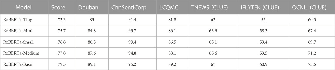
TABLE 1. Scores of the BERT model.
Pooling strategy: SBERT adds a pooling operation to the output of BERT/RoBERTa to generate a fixed-size sentence embedding vector. Three pooling strategies were adopted in the experiment for comparison.
1. Directly using the output vector of CLS position to represent the vector of the whole sentence.
2. MEAN strategy: The average value of each token output vector is calculated to represent the sentence vector.
3. MAX strategy: The maximum value of each dimension of all output vectors is taken to represent the sentence vector. Specific values are given in Table 2.
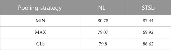
TABLE 2. Pooling strategy score.
Then, principal component analysis (PCA) was used for analysis. PCA is a common data analysis method, which is often used to reduce the dimension of high-dimensional data, and can be used to extract the main feature components of data. For industry types, the pre-trained BERT model is used to embed the text, and then, PCA is used to reduce the dimension.
3.3 PCA dimensionality reduction
Dimensionality reduction of high-latitude data can avoid the high complexity of the model caused by excessive data dimensions. Especially for some cases of insufficient sample data, the final trained model will have poor generalization. Removing the collinearity between data attributes can optimize the model, reduce the complexity of the model, reduce the training time of the model, and improve the robustness and generalization of the model. For PCA, this process is essentially a lossy feature compression process, but it is expected to lose as little accuracy as possible and retain the most original information in the compression process.
By setting text dataset ω, the feature after dimensionality reduction is A.
Because this task contains many influencing factors and the sample data are time series data, this task does not belong to a typical time series problem but should be classified as a multivariable time series problem. In this article, the existing problems will be transformed into supervised problems by using sliding time window so that the time series dataset can be suitable for supervised learning. The text data in the data are embedded with the BERT model, processed with PCA dimensionality reduction, and then, processed with the XGBoost regression model.
In the process of dimensionality reduction, the data after dimensionality reduction do not represent the advantages and disadvantages of the data after dimensionality reduction but reflect the distance of relevant industries. The reason is that this step extracts the more important components or key parts of the original data and maps them to another space. Currently, the performance of the data is not directly related to the original data, so there are positive and negative situations. The original data are compressed and transformed in the original space and mapped to a new space. In essence, it is the original data, but the form of expression is also different.
At this time, the dataset after defect filling, word embedding, and dimension reduction is recorded as X; then,
3.4 Data scaling
To prevent the model accuracy from being affected by abnormal data in the data, this article scales the data and limits the ROE to - 1–1.
where Q is the rate of ROE
The conversion method is
This transformation is often used as an alternative to zero mean, unit variance scaling. The task is not a typical time series problem, but a multivariable time series problem. By using sliding time window representation, time series datasets can be suitable for supervised learning. The idea of building a dataset is as follows:
First, the “securities code” column is used as the basis for grouping.
Second, the grouped data are sorted using “deadline.”
Third, the data of the previous n years are used to predict the “ROE in the N + 1 year.”
3.5 Feature selection
By selecting K Best, all features except the K features with the highest score are removed, and the function returns the variable score and p value. The calculation formula of p value is as follows:
In inferential statistics, hypothesis testing is a very important link. Through the statistical analysis of SAS and SPSS, it is found that p value (p value, probability, PR) is another important basis for testing.
3.6 ROE model
The ROE model is essentially the XGBoost model. XGBoost is a tree-based model. It can stack as many trees as possible, and each additional tree tries to reduce the errors of the previous tree set. The general idea is to combine many simple and weak predictors to build a powerful predictor.
XGBoost is an addition formula composed of multiple decision trees, which is expressed as follows:
where the estimated
Therefore, for each tree, the XGBoost model is essentially an additive model. We observe
The objective function of a given XGBoost is
where
Since the objective function is difficult to solve at this time, the Taylor formula can be used for an approximate solution.
where
After removing the constant term in the objective function, the simplified approximate function is obtained.
The previous formula is to calculate the loss for each sample
where
Since the loss function is convex, the partial derivative of the objective function can be obtained to find the minimum value point in the interval, which represents the case of minimum loss. After calculation, the expression of min(L) of the minimum loss value is
The formula is used to measure the quality of decision tree. Based on the given loss function, after pruning the decision tree, we observe whether the value of the loss function decreases to judge whether pruning should be performed.
The forward step-by-step algorithm is used for model optimization, and the objective function is
According to the XGBoost document, the equation is as follows:
In determining where each decision tree forks, the exact greedy algorithm is adopted.
Here,
Since the exact greedy algorithm affects the calculation efficiency when the sample size is large, the approximate algorithm can be used. Global and local methods can be used to determine the split point.
Global indicates that the candidate splits are calculated before the spanning tree. This method does only one operation in the whole calculation process. The candidate segmentation points that have been calculated in advance are used in the subsequent node division; local calculates the candidate segmentation points only when each node is divided. Experiments show that if the two methods want to achieve the accuracy of approaching the exact greedy algorithm, we need to take more candidate segmentation points to improve the accuracy. Because local needs to be calculated every time the node is divided, in some cases, the amount of calculation is very close. The use of the two methods is also different, which is suitable for taking a large number of segmentation points; local is more suitable for deep tree structures.
In order to avoid the unreasonable definition of candidate cut points by simple statistical indicators, the weighted quantile sketch is introduced.
Dataset
Ranking function
Then, candidate points are selected according to the following formula:
In terms of sparse values, the model can automatically learn the default division direction for the missing data. In each segmentation, the missing value is segmented to the left node and the right node. By calculating the score value and comparing which of the two segmentation methods is better, an optimal default segmentation direction will be learned for the missing value of each feature.
In a word, once the model is trained, the prediction simply boils down to identifying the correct leaves of each tree according to the characteristics and summarizing the value of each leaf, which becomes the most difficult part of the problem.
XGBoost is an optimal allocation gradient lifting program for efficiency, flexibility, and convenience. Based on gradient boosting, a machine learning method based on gradient boosting is completed. XGBoost provides a parallel tree structure (also known as GBDT, GBM) that can quickly and accurately deal with a large number of data science problems. XGBoost is an implementation of gradient lifting integration method for classification and regression problems. In this task, the sliding time window representation is used to make the time series dataset suitable for supervised learning.
3.7 Effect evaluation
The goodness of fit test of this model adopts the external data verification method; that is, the simulation test is carried out with the data not participating in the training in the sample data to verify the accuracy and stability of the model prediction. The data used to evaluate the link account for about 50% the total sample data.
After the XGBoost model is constructed, the model is scored with the data of the training set. Here, we need to pay attention to the scoring standard R2. XGBregressor is used for the score. Since it is a regression model, the scoring standard of the regression model should be selected.
Under this scoring standard, when the model is better, R2 → 1 and when the model is worse, R2 → 0.
4 Experimental process
4.1 Data source
The data in this article are from the Guotai’an database. A total of 12,072 corresponding indicators of 1,084 Chinese energy enterprises from 2003 to 2021 are selected for analysis. The selected variables are shown in Table 3.
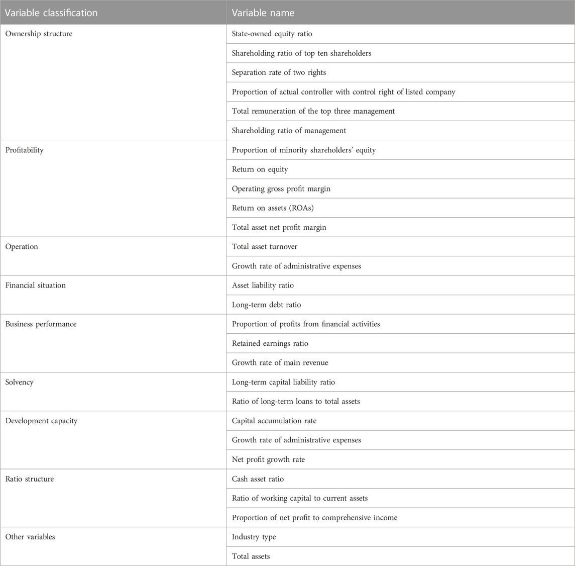
TABLE 3. Variable classification table.
According to the industry type, energy companies are divided into traditional energy, new energy, and energy reserve according to the energy type. The specific classification is shown in the table as follows.
The data are preliminarily screened, and descriptive statistics are carried out. The software is SPSS. The descriptive statistics of the data is given in Table 4.
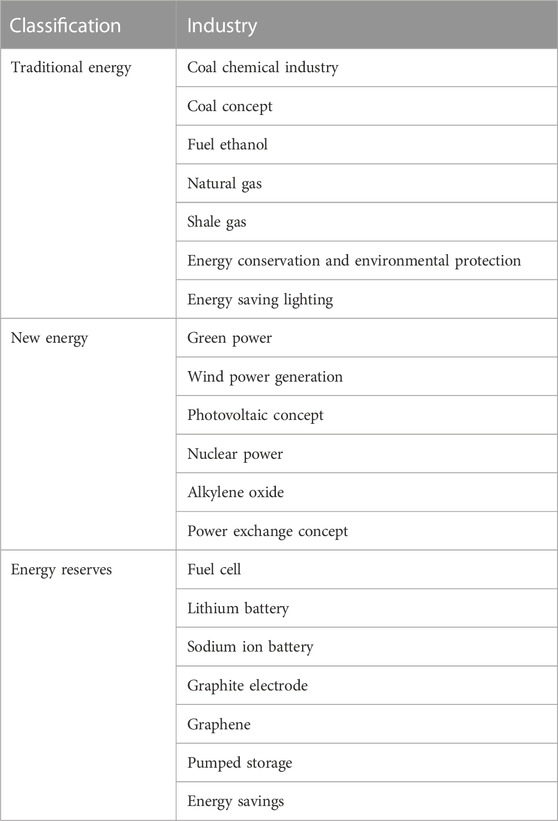
TABLE 4. Classification of energy enterprises.
It can be seen from Table 5 that the minimum value of the core explanatory variable enterprise performance ROE is −28.2046, maximum value is 204.6869, mean value is 0.04, and standard deviation is 2.11727, indicating that there are individual outliers, but the overall volatility is small and the data are relatively concentrated. The difference between the maximum and minimum values of the equity ratio of SOEs, long-term debt ratio, total asset turnover rate, retained earnings ratio, and the equity ratio of the top ten shareholders is less than 10, and the standard deviation is less than 1, indicating that its numerical distribution is uniform and concentrated, with little fluctuation. For the normal operation of the model data, this article first removes the enterprises with state-owned equity ratio of 0 before regression and removes the extreme values of other control scalars.
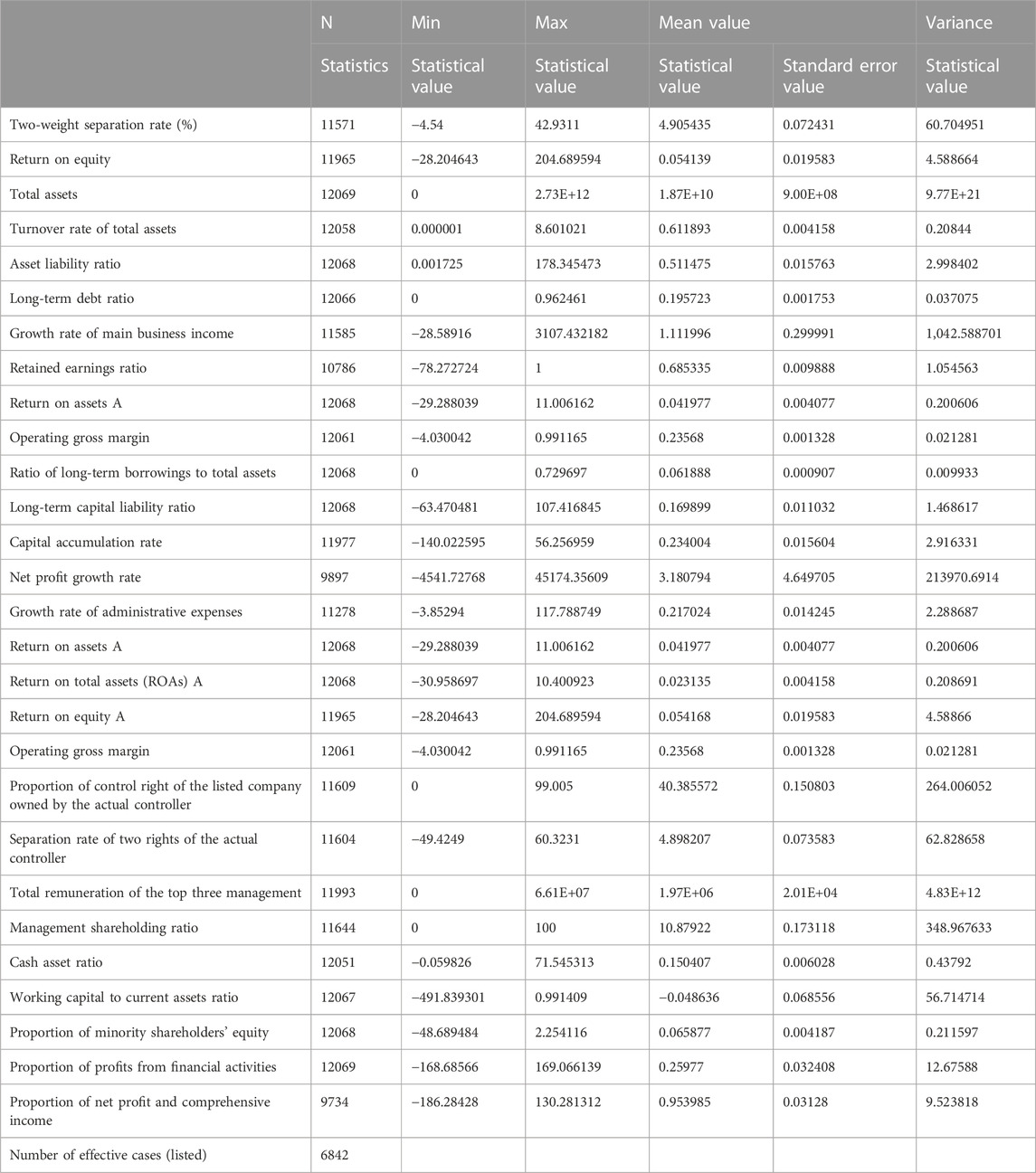
TABLE 5. Descriptive statistics.
4.2 Missing value supplement
The purpose of making up the missing values is to retain as much sample data as possible for the training of datasets. Once the missing values are not handled well, the analysis results may be unreliable and fail to achieve the purpose of analysis. However, not all data can be supplemented, and the supplemented data are not the real value of the data sample, but based on other existing fields, the missing field is predicted as the target variable, so as to obtain the most possible complement value.
For example, in Figure 1, in the missing value statistics, there are 1,283 missing data values of the variable “retained earnings rate,” and the missing values of the variable are in the middle of the 18-year time span, which has a strong regularity. This depends on the nature of the variable itself. In terms of profit distribution, many enterprises distribute profits due to established strategies, in the development period or quota. Therefore, the index data will show the same value for many years, with strong regularity and in line with the continuity of time. Therefore, the k-value complement method can be used to supplement the data.

FIGURE 1. Supplementary effect drawing of retained earnings.
Thus, the sample data can be retained as much as possible to realize the full application of the sample data, so as to form a complete data record for subsequent data processing and analysis.
4.3 Word embedding
Word embedding for text types: The main idea of word embedding is to transform the text into a vector representation of lower-dimensional space. There are two important requirements for this transformed vector: lower-dimensional space and minimizing the sparsity of the encoded word vector. This article uses the BERT model for word embedding. The BERT model used in this article is shown in Figure 2.

FIGURE 2. Flow chart of the BERT model.
4.4 PCA dimensionality reduction
The data obtained after word embedding are high-latitude data, so PCA is used for analysis. PCA is a common data analysis method, which is often used to reduce the dimension of high-dimensional data, and can be used to extract the main feature components of data. For industry types, the pre trained BERT model is used to embed the text, and then, PCA is used to reduce the dimension.
PCA is essentially a lossy feature compression process, but it is expected to lose as little accuracy as possible and retain the most original information in the compression process. In this model, the variable “industry type” belongs to text variable, which cannot be quantified intuitively. Therefore, we build the BERT model to embed text words into the classified variable “industry type,” so as to obtain a large number of high-dimensional data. PCA is used to reduce the dimension of the obtained high-dimensional data. Treatment results are given in Table 6. The corresponding scatter diagram is shown in Figure 3.
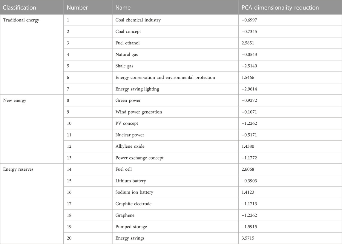
TABLE 6. PCA data dimensionality reduction result.

FIGURE 3. Scatter diagram of dimension reduction results of PCA.
The data in the aforementioned chart represent the distribution of industries. The sign does not represent the advantages and disadvantages of the data, but reflects the distance of relevant industries. The reason is that after extracting the more important components or key parts of the original data in this step, they are mapped to another space. At this time, the performance of the data is not directly related to the original data, so there are positive and negative situations. The original data are compressed and transformed in the original space and mapped to a new space. In essence, they are the original data, but the form of expression is different.
4.5 Data zoom
The multi-index comprehensive evaluation method is scientific and reasonable to evaluate things. It combines multiple indexes describing different aspects of a thing to get a comprehensive index and evaluates and compares the thing through it. Due to different properties, different evaluation indexes usually have different dimensions and orders of magnitude. When the indexes differ greatly, if the original index value is directly used to calculate the comprehensive index, the role of the index with larger value in the analysis will be highlighted and the role of the index with smaller value in the analysis will be weakened.
Data scaling, in statistics, means that the original data are converted according to a certain proportion through a certain mathematical transformation method, and the data are placed in a small specific interval. The purpose is to eliminate the differences of characteristic attributes such as characteristics and quantity between different samples and convert them into a dimensionless reactive value. The characteristic quantity values of each sample are in the same order of magnitude.
As shown in Figure 4, after excluding the extreme value, this article scales the ROE to
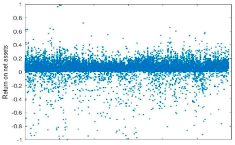
FIGURE 4. Scatter chart of return on equity scaling results.
4.6 Eigenvalue selection
Eigenvalue selection is very important. Some scholars believe that in most machine learning tasks, features determine the upper limit of model effect, and the selection and combination of models are only infinitely close to this upper limit.
Feature selection can reduce the number of features, prevent dimension disaster, and reduce training time. The generalization ability of the model is enhanced, and overfitting is reduced; the understanding of features and eigenvalues is enhanced. Specific data are given in Table 7. In this article, the eigenvalues are selected according to the p value, and the results are as shown in Figure 5.
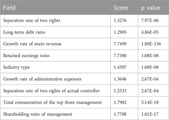
TABLE 7. Statistical table of p value score.
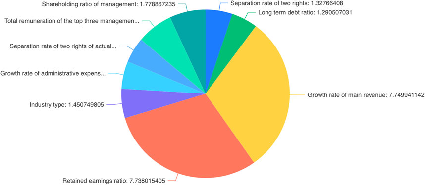
FIGURE 5. Variable score pie chart.
The smaller the score in the aforementioned table, the better it can reflect the correlation between independent variables and dependent variables. Among the top ten of the aforementioned eigenvalues, the impact of equity specific factors is the first, which means that equity factors play an important role in the prediction of ROE.
It can be seen from the aforementioned table that the score of the two rights separation rate is the lowest, so the cash capital ratio has the lowest impact on the ROE, and the two rights separation rate has the greatest impact on the ROE.
It can be seen from the aforementioned pie chart that the p value of the separation rate of the two rights is the highest, and the equity factors stand out among several other factors, which has the greatest impact on the prediction rate of the ROE.
4.7 Construction of the equity net asset return model
The ROE equity model is essentially the XGBoost model. XGBoost is a tree-based model. It can stack as many trees as possible, and each additional tree tries to reduce the errors of the previous tree set. The general idea is to combine many simple and weak predictors to build a powerful predictor.
After construction, the results of the equity net asset income model are as shown in Figure 6.
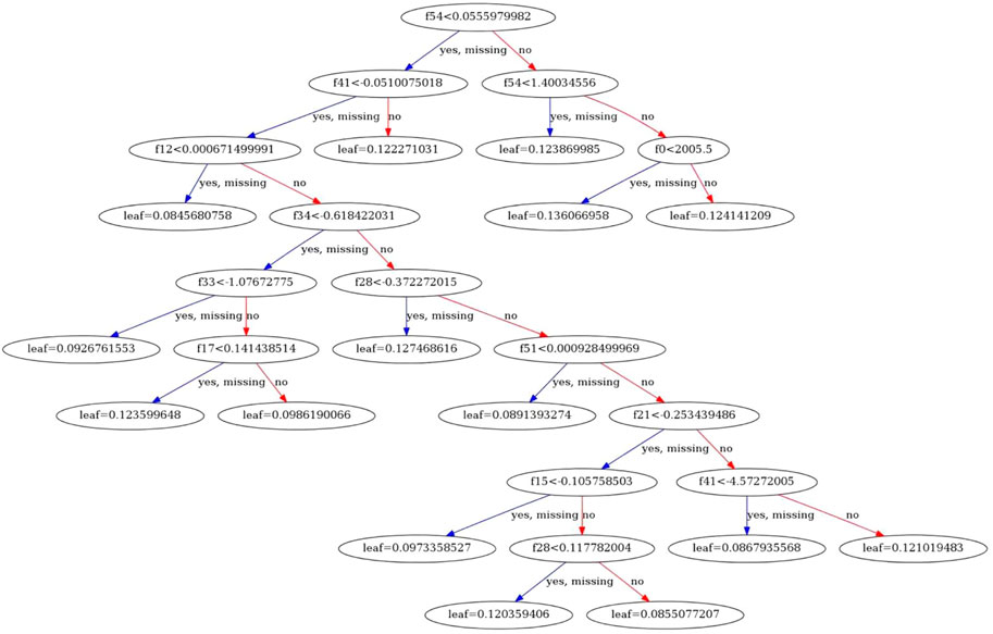
FIGURE 6. Schematic diagram of the XGBoost model.
The model is the final result of the collection of multiple decision trees. The red line is the branch reduction direction of the decision tree, and the blue line is the decision direction of the decision tree.
4.8 Model evaluation
The goodness-of-fit test of this model adopts the external data verification method; that is, the simulation test is carried out with the data not participating in the training in the sample data to verify the accuracy and stability of the model prediction. The data used to evaluate the link account for about 50 percent of the total sample data.
After the XGBoost model is constructed, the model is scored with the data of the training set. Here, we need to pay attention to the scoring standard R2. XGBregressor is used for score. Since it is a regression model, the scoring standard of the regression model should be selected. Under this scoring standard, when the model is better, R2 → 1 and when the model is worse, R2 → 0.
Finally, under this scoring standard, through the evaluation of the model, the final score of the model is
The score shows that the independent variable of this model has a good explanation for the dependent variable, so the ROE predicted 435 by this model is reliable.
4.9 Model comparison
After the previous experiments and conclusions, this section will now conduct comparative experiments and compare R2 scores of different machine learning model methods.
The datasets that have been processed are brought into the decision tree regression model, the BP neural network model, and the random forest regression model, and the R2 scores of each model operation are obtained as shown in Table 8, with the scores of 0.921, −0.0071, and 0.861. This value is less than 0.946 of the model R2 in our model. Therefore, among these models, the model built in this article has the highest accuracy.
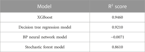
TABLE 8. Model score comparison.
5 Conclusion
Using the XGBoost model, this article constructs the net asset income model of energy enterprises based on the characteristics of ownership structure through missing value supplement, word embedding, PCA dimensionality reduction, and model evaluation. After evaluation, the data accuracy of the N + 1 year predicted by the model based on the data of the previous n years is about 95%, and the prediction effect is good.
Under the background of carbon neutralization and carbon peak, the operation status of energy enterprises is gradually remarkable. With the rapid development of energy enterprises, the ownership structure is becoming more and more complex. Taking energy enterprises as the research object and based on the XGBoost model, this article constructs the ROE equity model to realize the accurate, scientific, and timely prediction of the ROE and can reasonably modify and allocate the equity structure of energy enterprises through the predicted ROE, so as to play the role of prediction and early warning for the next business cycle of enterprises. The timeliness of the prediction of the ROE of this model can reasonably avoid the lag of the ROE and play a positive role in the equity planning and future development of energy enterprises.
At present, the relationship between equity and ROE generally tends to be inter-industry research, which is not subdivided into different types in a specific industry. In addition, the existing research is more inclined to analyze the existing results, that is, to analyze the connection in the existing data at a certain time node, which has a certain lag effect, which is caused by the lag of the ROE itself.
The aforementioned research ideas are not scientific in predicting the future business performance level, and the test cycle of the conclusions is long. To sum up, this article abstracts the problem into a multivariable time series problem by using the thought and method of deep learning, analyzes it under various indicators, scientifically and effectively predicts the operation effect of the next cycle in this business cycle, and modifies the equity proportion and rights by predicting the ROE, so as to achieve a more ideal and reasonable level.
ROE is the most important financial indicator in the business process of an enterprise, and it is also the benchmark to judge whether the business is healthy or not. Many enterprises hope to achieve the performance indicators, so the research on ROE has always been the favorite of different scientists. Based on XGBoost, this article uses missing value supplement, PCA dimensionality reduction, and the BERT model to process text information, uses the R2 score method to evaluate the model, takes energy enterprises in multiple industries as samples to process and predict multivariate time series data, and adds comparative experiments. The experiment shows that the prediction accuracy of this model is higher than that of other machine learning models, and the dataset can be directly applied to this model after adding text variables, which increases the range of variables compared with other machine learning models, and can better predict the ROE of energy enterprises. In addition, this model is not only limited to predicting the ROE of energy enterprises but also applicable to other types of enterprises. Compared with the traditional regression model, this model has certain advantages, mainly focusing on two points: first, the focus is different. Traditional regression models pay more attention to the coefficient relationship between various indicators and ROE, that is, the change trend; the model in this article is more direct to get the predicted value, and the data are more secure because they come from a lot of learning. Second, the traditional regression model is not good at dealing with text information. This model takes this factor into account and is not bound by reasonable text variables. Third, the model proposed in this article has more advantages for processing large amounts of data and seeing the general changes of the whole industry.
Data availability statement
The original contributions presented in the study are included in the article/Supplementary Materials, further inquiries can be directed to the corresponding author.
Author contributions
YY: data analysis, writing, and formal analysis. ZW: validation and methodology.
Conflict of interest
The authors declare that the research was conducted in the absence of any commercial or financial relationships that could be construed as a potential conflict of interest.
Publisher’s note
All claims expressed in this article are solely those of the authors and do not necessarily represent those of their affiliated organizations, or those of the publisher, the editors, and the reviewers. Any product that may be evaluated in this article, or claim that may be made by its manufacturer, is not guaranteed or endorsed by the publisher.
References
Arviyanti, A., and Muiz, E. (2020). Pengaruh karakeristik perusahaan dan struktur kepemilikan terhadap penghindaran pajak/tax avoidance pada perusahaan bumn yang terdaftar pada bei tahun 2013-2016. J. Akunt. 7 (1), 28–46. doi:10.37932/ja.v7i1.22
Bhattarai, D. (2018). Generic strategies and sustainability of financial performance of Nepalese enterprises. PRAVAHA 24 (1), 39–49. doi:10.3126/pravaha.v24i1.20224
Bіelіenkova, O. (2020). Factor analysis of profitability (losses) construction enterprises in 1999-2019.
Chazova, I. Y., and Mukhina, I. A., Effectiveness of administration of economic entities in state and municipal ownership, In Proceedings Of The International Science And Technology Conference "Fareastсon" (Iscfec 2019), 2019.
Farooq, U. (2019). Impact of inventory turnover on the profitability of non-financial sector firms in Pakistan. J. Of Finance And Account. Res. 01, 34–51. doi:10.32350/jfar.0101.03
Gao, L., and Song, S. (2021). Determining the problems of management shareholding and the mixed ownership, modern perspectives in economics. Bus. And Manag. 7.
Gao, T., Yang, X., Ren, Z., and Zhao, J. (2022). Research on non-contact heart rate detection method based on GP-XGBoost. OTHER Conf.
Irfan Sauqi, M., Endah, T. W., and Heni, A. (2019). Analisis kinerja keuangan terhadap harga saham pada industri loga yang terdaftar di bei. EQUITY 22, 37–46. doi:10.34209/equ.v22i1.899
Ji, H. P., and Kim, C. Y. (2020). Social enterprises, job creation, and social open innovation. J. Open Innovation Technol. Mark. Complex. 6 (4), 120. doi:10.3390/joitmc6040120
Mao, Z., Xia, M., Jiang, B., Xu, D., and Shi, P. (2022). Incipient Fault diagnosis for high-speed train traction systems via stacked generalization. Ieee Trans. Cybern. 52, 7624–7633. doi:10.1109/tcyb.2020.3034929
Matuszak, P., and Szarzec, K. (2019). The scale and financial performance of state-owned enterprises in the CEE region. ACTA OECONOMICA 69, 549–570. doi:10.1556/032.2019.69.4.4
Men, T. B., and Hieu, M. N. (2021). Determinants affecting profitability of firms: A study of oil and gas industry in Vietnam. J. Of Asian Finance, Econ. And Bus.
Nar, B. B., Nitesh, R. B., Om, S., Pooja, G., Poshan, L., Pratiksha, P., et al. (2018). Impact of corporate governance on dividend policy of Nepalese enterprises. Bus. Gov. And Soc., 377–397. doi:10.1007/978-3-319-94613-9_21
Nguyen, N. H., Abellán-García, J., Lee, S., García-Castaño, E., and Vo, T. (2022). Efficient estimating compressive strength of ultra-high performance concrete using XGBoost model. J. Of Build. Eng. 52, 104302. doi:10.1016/j.jobe.2022.104302
Otekunrin, A. O., Nwanji, T. I., JohnsonOlowookere, K., Egbide, B-C., Fakile, S. A., Lawal, A. I., et al. (2018). Adebanjo joseph falaye, damilola felix eluyela, financial ratio analysis and market Price of share of selected quoted agriculture and agro-allied firms in Nigeria after adoption of international financial reporting standard. J. Of Soc. Sci. Res.
Petruk, O., Trusova, N., Polchanov, A., and Dovgaliuk, V. (2020). The influence of the capital structure on the efficiency of communal enterprises of passenger transport. Mod. Econ. 24 (1), 132–137. doi:10.31521/modecon.V24(2020)-21
Roffia, P. (2021). Family involvement and financial performance in SMEs: Evidence from Italy. Int. J. Of Entrepreneursh. And Small Bus. 43, 39. doi:10.1504/ijesb.2021.115313
Sanyal, R., Kar, D., and Sarkar, R. (2022). Carcinoma type classification from high-resolution breast microscopy images using A hybrid ensemble of deep convolutional features and gradient boosting trees classifiers. Ieee/Acm Trans. Comput. Biol.
Shen, Z., AhmedDeifalla, F., Kamiński, P., and Dyczko, A. (2022). Compressive strength evaluation of ultra-high-strength concrete by machine learning. MATERIALS 15 (10), 3523. doi:10.3390/ma15103523
So, Y. K., Shin, H-H., and Yu, S. (2018). Do state-owned enterprises cooperate with suppliers? Performance analysis in the Korean case. Emerg. Mark. Finance And Trade 15.
Srinivas, P., and Katarya, R. (2022). HyOPTXg: OPTUNA hyper-parameter optimization framework for predicting cardiovascular disease using XGBoost. Biomed. SIGNAL Process. CONTROL.
Tho Do, T. (2020). The relationship between capital structure and firm performance: The case of Vietnam material enterprises. Res. J. Of Finance And Account.
Ullah, I., Liu, K., Yamamoto, T., Zahid, M., and Jamal, A. (2022). Prediction of electric vehicle charging duration time using ensemble machine learning algorithm and shapley additive explanations. Int. J. ENERGY Res. 46, 15211–15230. doi:10.1002/er.8219
Vlčková, M., Frantíková, Z., and Vrchota, J. (2019). Relationship between the financial indicators and the implementation of telework, DANUBE: Law. Econ. And Soc. Issues Rev.
Wang, Y., and Zhao, D. (2021). “Research on the evaluation index system of trust, innovation and M&A value,” in Proceeding of the Journal Of Physics: Conference Series.
Yang, Y., Wang, K., Zhen, Z. Y., and Liu, D. (2022). Predicting freeway traffic crash severity using XGBoost-bayesian network model with consideration of features interaction. J. Of Adv. Transp. 2022, 1–16. doi:10.1155/2022/4257865
Zhang, C., Hu, D., and Yang, T. (2022). Anomaly detection and diagnosis for wind turbines using long short-term memory-based stacked denoising autoencoders and XGBoost. Reliab. Eng. Syst. Saf.
Zhou, N. (2018). Hybrid state-owned enterprises and internationalization: Evidence from emerging market multinationals. Manag. Int. Rev. 58, 605–631. doi:10.1007/s11575-018-0357-z
Keywords: energy industry, equity, return on equity, XGBoost, predict
Citation: Yang Y and Wang Z (2023) Prediction of return on equity of the energy industry based on equity characteristics. Front. Energy Res. 11:1136914. doi: 10.3389/fenrg.2023.1136914
Received: 03 January 2023; Accepted: 15 March 2023;
Published: 28 March 2023.
Edited by:
Zbigniew M. Leonowicz, Wrocław University of Technology, PolandReviewed by:
Najabat Ali, Hamdard University, PakistanMengshi Li, South China University of Technology, China
Copyright © 2023 Yang and Wang. This is an open-access article distributed under the terms of the Creative Commons Attribution License (CC BY). The use, distribution or reproduction in other forums is permitted, provided the original author(s) and the copyright owner(s) are credited and that the original publication in this journal is cited, in accordance with accepted academic practice. No use, distribution or reproduction is permitted which does not comply with these terms.
*Correspondence: Zhenqing Wang, d2FuZ3poZW5xaW5nMTEyOEAxNjMuY29t