
94% of researchers rate our articles as excellent or good
Learn more about the work of our research integrity team to safeguard the quality of each article we publish.
Find out more
ORIGINAL RESEARCH article
Front. Energy Res., 03 April 2023
Sec. Solar Energy
Volume 11 - 2023 | https://doi.org/10.3389/fenrg.2023.1118654
This article is part of the Research TopicRising Stars in Energy Research: 2022View all 10 articles
 Paolo Graniero1,2
 Mark Khenkin1*
 Hans Köbler3
 Noor Titan Putri Hartono3
 Rutger Schlatmann1
 Antonio Abate3
 Eva Unger4
 T. Jesper Jacobsson5
 Carolin Ulbrich1
Perovskite solar cells are the most dynamic emerging photovoltaic technology and attracts the attention of thousands of researchers worldwide. Recently, many of them are targeting device stability issues–the key challenge for this technology–which has resulted in the accumulation of a significant amount of data. The best example is the “Perovskite Database Project,” which also includes stability-related metrics. From this database, we use data on 1,800 perovskite solar cells where device stability is reported and use Random Forest to identify and study the most important factors for cell stability. By applying the concept of learning curves, we find that the potential for improving the models’ performance by adding more data of the same quality is limited. However, a significant improvement can be made by increasing data quality by reporting more complete information on the performed experiments. Furthermore, we study an in-house database with data on more than 1,000 solar cells, where the entire aging curve for each cell is available as opposed to stability metrics based on a single number. We show that the interpretation of aging experiments can strongly depend on the chosen stability metric, unnaturally favoring some cells over others. Therefore, choosing universal stability metrics is a critical question for future databases targeting this promising technology.
New photovoltaic technologies are urgently needed to accelerate the adoption of affordable renewable energy sources and combat climate change. Perovskite solar cells (PSCs) represent a prime candidate technology, which has become the most dynamic research area in photovoltaics. Researchers have obtained power conversion efficiency (PCE) values of over 25% in a single junction device (Green et al., 2022) and over 32.5% in tandems with silicon (‘Best Research-Cell Efficiency Chart’ n.d.) thanks to perovskite compositional engineering, deposition techniques optimization, and device architecture adjustments. Despite this highly competitive efficiency compared to silicon and the low manufacturing costs, there are still barriers to the commercialization of halide perovskites. Operational stability is the most prominent and, therefore, the focus of the data analysis in this work.
Currently, the lifetime of perovskite solar devices remains well below the target value of 25–30 years (i.e., more than 200,000 h); Figure 1 shows the average lifetime of perovskite solar devices published in scientific papers over the period 2013 to February 2020 (i.e., the period considered in the Perovskite Database project, see below), clearly showing the need to improve the operational stability of these devices. The factors that have contributed so far to improvements in PSCs stability from hours to months are, for example, perovskite compositional engineering (Chi and Banerjee, 2021; Mazumdar, Zhao, and Zhang, 2021), the introduction of passivation (Chen et al., 2019) and blocking (Brinkmann, Gahlmann, and Riedl, 2020) layers, optimization of transport (Foo et al., 2017; Xinxing Yin et al., 2020; Dipta and Uddin, 2021) and contact (Nath et al., 2022) layers, and device encapsulation (Lu et al., 2021).
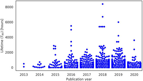
FIGURE 1. Lifetime T80 in hours of every perovskite solar device published between 2013 and February 2020 (for which T80 was reported in the Perovskite Database). The vast majority of devices reported, 1,790 out of 1,834, have a short lifetime of at most 2,000 h.
With thousands of researchers worldwide dedicating their efforts to studying PSCs, an individual researcher has no chance of keeping track of all these results. Combining the device data produced during the experiments in shared databases offers significant benefits. The abundance of data allows the application of statistical techniques, most notably machine learning (ML), to empower data-driven research activities and for gaining new insights that would be otherwise impossible to obtain by analyzing data from individual studies only. Several authors have already pointed at ML as one important tool in overcoming challenges (Myung et al., 2022) in perovskite research, for example, screening of suitable candidate materials for photovoltaic applications (Chen et al., 2022), or to use data extracted from scientific publications to characterize the performance of PSCs (Liu et al., 2022). Thus far, few authors have attempted to use shared data to examine the stability of perovskite solar cells (Beyza Yılmaz and Ramazan Yıldırım, 2021). Even fewer authors used shared experimental data: Tiihonen et al. (2018) studied a set of 261 aging tests to assess the quality of published stability data, finding several issues in how the authors reported the results of their studies at the time; Çağla Odabaşı and Ramazan Yıldırım (2020) applied ML to a data collection of 404 aging tests data to derive the effects of perovskite composition and transport layers on the PSCs stability, concluding that the analysis of data collected from the literature can be beneficial to better understand the overall state of the literature and for gaining insights about high stability devices.
Collecting the data from publications represents a tremendous effort which explains the lack of studies in this direction. Notably, the “Perovskite Database Project” was recently released (Jacobsson et al., 2022) (www.perovskitedatabase.com). This publicly open database contains manually extracted data from more than 15,000 publications with keywords “perovskite solar” from the Web of Science until February 2020. It holds information about more than 42,400 devices, 1,834 of which contain measured T80 (i.e., the time it takes for a device to lose 20% of its initial efficiency). The Perovskite Database is not only a much larger dataset than any other previously put together, but it also attempts to collect the most detailed information: the authors collected more than 400 parameters in the database, which include information about the cells’ design, the functional layers of the device stack, the details of device synthesis and key metrics about efficiency, stability, and outdoor performance.
Even though this dataset is the largest so far, the quality of stability-related data is a concern. Some aspects of particular relevance are the number of missing values due to incomplete reporting in the source publications, the low statistical relevance of data entries which report only the best-performing devices and an incomplete set of experimental results, and the need to stick to standardized guidelines for the aging conditions to improve comparability. This work is a first attempt at applying ML to the stability data in the Perovskite Database to identify relevant factors affecting device stability. However, the performance of the models turns out to be unsatisfactory. To understand if this low performance is due to the small database size or data quality issues introduced above, we perform computational experiments using the concept of learning curves. This tool allows us to extrapolate the performance of the ML models to more extensive databases that we expect will be available in the future. We want to show how data quality, specifically regarding the number of missing values, impacts the performance of ML models used to study perovskite stability. We further use the concept of learning curves to estimate how much the performance of an ML model would increase by collecting more data, as a function of data quality.
Importantly, even with a much larger dataset, there is another potentially critical issue with tabular data where a single number represents device stability. Aging experiments typically record the evolution of power conversion efficiency (PCE) or other device parameters under different stress conditions. Unlike PCE, a highly standardized figure of merit (FOM) of device performance, there is no generally accepted figure of device stability that would reduce the time series from aging experiments to a single number in a tabular database. T80 is one of the most common stability metrics, working sufficiently well for solar technologies that show uniform degradation curves. T80 is reported in the Perovskite Database and was used in this work as the target variable for ML modeling. To study the adequacy of this metric, we use an in-house dataset that includes complete time series from more than 1,000 aging experiments, which were recorded in a custom-built setup (Köbler et al., 2022) in the years 2019–2022. We show that there are diverse aging behaviors resulting in a variety of time-series shapes. We computed different FOMs used in the PSCs literature (Khenkin et al., 2020; Almora et al., 2021) to all these curves, showing that they poorly correlate with each other, given the variety of degradation behaviors. This lack of correlation shows the urgent need to define a “fair” FOM for device stability. This fair FOM would then empower data-driven research activities on the stability of PSCs, providing a meaningful, universal, accurate, and precise stability measure. The definition of this fair FOM of stability and the production of more complete data regarding aging experiments can significantly accelerate the development of commercially viable perovskite solar devices through ML methods.
We used two large datasets in the analyses presented in this work. The first one is the Perovskite Database, based on the data extracted from the literature. It contains information on a wide variety of device architectures and aging conditions. The other dataset originates from in-house aging experiments and contains fewer details but provides full aging curves. The latter is only used to discuss the issue of selecting a FOM to characterize device stability.
The Perovskite Database Project contains data manually collected from more than 15,000 papers about perovskite solar cells. The manual scraping of the publications resulted in collecting information about more than 42,400 perovskite solar devices.
The data categories, or features, contained in the Perovskite Database include reference data about the source publication, properties of the cell (e.g., area, architecture), data for every functional layer in the device stack, about the synthesis of the cell, and key metrics (e.g., stability, JV metrics, outdoor performance). The database’s total number of features (i.e., the number of columns) is 409.
This dataset represents the most extensive collection of published experimental data about perovskite solar devices. Out of more than 42,400 devices reported in the database, only 1,834 include measured T80 values. In principle, we could use the PCE at the end of the stability experiments and the length of such experiments to extrapolate the value of T80 for instances in which it has not been reported. We refrain from doing this because, as we show in this work using the in-house dataset, the wide variety of aging behaviors would make such extrapolation highly uncertain.
Note that, in this study, we selected a subset of 67 out of the 409 features in the database based on expert knowledge about the factors most likely to affect the stability of the devices.
The in-house dataset (collected in the Department “Active Materials and Interfaces for Stable Perovskite Solar Cells” at Helmholtz-Zentrum Berlin) contains time-series data of aging experiments performed on over 1,000 perovskite solar cells of various types in the years 2019–2022. This dataset is the largest of this type used in a publication. Cells were aged in a custom-built high-throughput aging system (Köbler et al., 2022) under continuous illumination of a metal-halide lamp. Special electronics are employed to MPP-track every solar cell individually. Experiments are performed under nitrogen atmosphere at room temperature or at elevated temperatures according to ISOS-L1I or ISOS-L2I (Khenkin et al., 2020). The time exposure of experiments ranges between 150 and 2,060 h. The exact experimental conditions are less relevant to our goals since we want to compare how different FOMs for stability correlate with each other for the same curve when computed automatically. Figure 2 shows an example of aging curves.
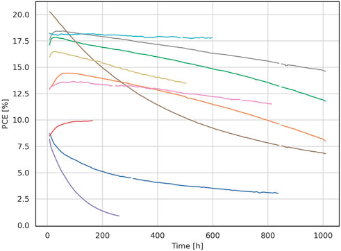
FIGURE 2. Example of time series data from the in-house aging experiments dataset. Each curve represents the aging of a different PSC (PCE evolution over time), showing the variety of behaviors in the aging of PSCs.
In the following subsections, we briefly describe how we prepared the data for analysis and the methods and concepts used to perform the analysis. More detailed information could be found in the Supplementary Material. The overall structure of the experiments is depicted schematically in Figure 3.
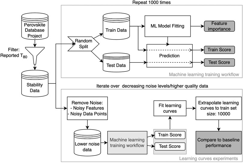
FIGURE 3. Schematic representation of the experiments performed.
Since the data in the Perovskite Database Project was collected by manually extracting information from scientific publications and manually writing the information to the database, some errors can be present. For example, there might be spelling errors in the names of chemical compounds and manufacturing techniques, or numerical values might be incorrect. We have not attempted to identify potential input errors in the numerical values of the features (i.e., we did not perform outlier detection or additional checks for numerical features), but we attempted to correct spelling and text formatting errors.
We have prepared the data in the Perovskite Database encoding every column of the dataset in numerical format, splitting columns that contained multiple simple features (e.g., device stack containing several layers), converting categorical values into dummy binary variables, and flagging missing values (NaNs) into additional columns.
Machine learning can be used with different goals in mind based on what knowledge we try to extract from the data: patterns, explanations, and predictors. Studies like (Odabasi and Yildirim, 2020) for PSC and (David et al., 2020) for organic PV try to find explanations, that is, explain how a given variable, like lifetime, is affected by properties of the devices. In the ML literature, the properties are generally referred to as features. Feature importance analysis refers to identifying a group of features with a significant impact on the target variable, in our case, T80.
There are different ways to study feature importance. In this work, we use the embedded method: we fit an ML model to the dataset and use measures of feature importance embedded in the model to study which factors affect stability the most. We explored several models (see Supplementary Material and Supplementary Figure S3) and selected two of them: Elastic Net (eNet), which is a linear model, and Random Forest (RF), which is a non-linear model. These represent the two broadest classes of ML models we can consider: they assume a linear or a non-linear relationship between the input features and the target variable, respectively.
Feature importance in eNet can be derived from the coefficients of the fitted model: the larger the magnitude of the coefficient of a feature, the higher the importance of that feature. For RF, a feature importance measure can be obtained during the training process by looking at the decrease in impurity in the trees that form the forest. Details about this can be found in (James et al., 2013).
When performing a feature importance analysis, it is necessary to consider how well the model can capture the patterns in the data, i.e., the goodness of fit. This is done by analyzing the model’s coefficient of determination, also called R2-score. The closer this coefficient is to 1, the better the goodness of fit of the model (the Supplementary Material contains the mathematical definition of the coefficient of determination).
Repeating the computation of the R2 score and feature importance value for multiple possible realizations of train and test set returns probability distributions instead of single values. We perform 1,000 draws of the train and test sets, keeping 75% of the data in the train set. We have considered both the whole dataset and two relevant subsets of the data: aging in the dark most of the time results in much longer lifetimes compared to photo-stability experiments; we, therefore, split the dataset into “Dark testing” and “Light testing” (refer to aging tests in the dark and under illumination). We also removed features related to the performance of the PSCs, like the initial PCE. While there is a statistical correlation between device efficiency and stability, it might reflect, for example, that simultaneous progress was made in these two critical aspects of the technology. In this work, we focused on the analysis of the impact of the device structure and parameters of ageing experiments.
Fundamental quantities in ML analysis are train and test errors. The train error measures the discrepancy between the values estimated by the ML model and the actual values of the target variable for the data in the train set, while the test error measures the same type of discrepancy but for the data in the test dataset. Since the train set is used to optimize the parameters of the models while the test set contains unseen data, the test error gives a reasonable estimation of the actual performance of the ML model. Additional details can be found in the Supplementary Material.
Following the definition in (Cortes et al., 1993), by learning curves, we mean the expected values of the test and training error as a function of the size of the training set; the expected value is taken over all the possible ways of choosing a training set of a given size.
Figure 4 schematically shows typical learning curves for a given model on a given dataset. If the model is sufficiently flexible (i.e., can learn a large number of functions) and the train set is relatively small, the training error will be very low, even zero: the model can perfectly fit the train set. In this case, the test error will be very high since it is highly likely that the model perfectly fitting the train set has learned not to model the data-generating process but the random noise present in the train set. As the size of the train set increases, the training error grows: the model learns more about the data-generating process from the available data, while the random noise is disregarded; at the same time, the test error decreases since the model becomes better at modeling the data and not the noise. In the limit of infinite train set size, training and test error converge to a common value
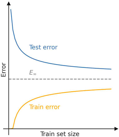
FIGURE 4. Schematic of the general behavior of learning curves for a given ML model.
From theoretical arguments (Seung, Sompolinsky, and Tishby, 1992), the learning curves can be modeled as power-law decays to the asymptotic error
We use learning curves to estimate the performance of our ML model in the hypothetical case in which a larger train set size becomes available. The learning curves (and the limiting performance) depend on the quality of the data. To simulate different data quality levels, we perform the learning curves experiments in three different settings:
• using the complete dataset in its original form;
• removing noisy features from the dataset;
• removing noisy data points from the dataset.
We start removing features or data points with the most missing values, therefore containing more noise, and iteratively less noisy ones, one at a time for the features, or allowing only a certain amount of missing values per data point in the third setting.
We perform the learning curves experiments for the complete dataset and data quality levels. We compute the learning curves for every dataset at ten different, increasing values of the training set size. To obtain the interpolation points, we average the results of a 20-fold cross-validation (sampling each train set 20 times) for each train set size. We then extract the parameters of the underlying power law function and extrapolate up to a train set size of 10,000 data points. The last step compares the estimated error values on such a hypothetical dataset with the extrapolated value obtained using the complete dataset.
In all learning curves experiments, we use Gradient Boosting as model, which performs similarly to Random Forest in modeling the dataset but has resulted in more stability during the training process; that is, the power law approximation is more accurate.
Figures of merit for perovskite stability are numerical values used to quantify the stability of the perovskite solar cells. Several different FOMs exist in the field. The most commonly used is T80, which represents the time it takes for the cell to lose 20% of its initial PCE. T80 has been successfully used with silicon-based photovoltaic technology since the aging behavior of such devices is relatively simple (in many cases, close to linear), and the aging behavior is well captured by T80. This is not necessarily the case for emerging PV technologies. For example, for organic photovoltaics typical shape has a fast initial decay (“burn-in”) followed by a linear decrease in efficiency, and an adapted metric called “stabilized T80”is more common (Roesch et al., 2015).
In contrast, PSCs show a variety of aging behaviors. This variety is reflected in the lack of a universally accepted FOM for their stability. For example, T80 alone has at least three different definitions based on the type of aging behavior and authors’ preferences (Khenkin et al., 2020), as illustrated in Figure 5.
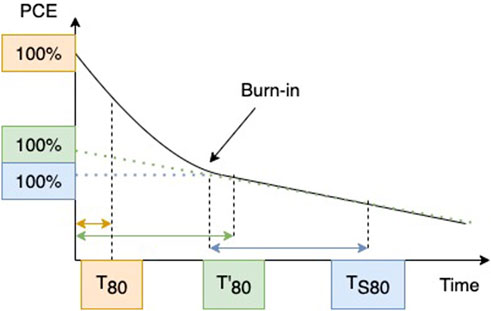
FIGURE 5. Three different definitions of T80 for an aging time series. The reported T80 varies depending on the chosen definition. Adapted from (Khenkin et al., 2020).
Since all the FOMs are used to quantify the same concept, e.g., stability, ideally, we want all of them to, at least qualitatively, agree: if a given device is more stable than another according to one FOM, it should also be more stable according to other FOMs. In order to confirm whether different FOMs for perovskite stability agree, we have used our in-house dataset of time-series data produced during aging experiments. We have defined different FOMs:
• T80: The time it takes for the PCE to drop 20% from the value at the beginning of the experiment.
• T’80: The time it takes for the PCE to drop 20% from the back-extrapolated value at the beginning of the experiment; back-extrapolation performed with a linear function, starting after the burn-in point.
• TS80: The time it takes for the PCE to drop 20% from the value at the burn-in point
• % PCE after X hours: Fraction of the initial PCE measured after X hours.
• Degradation rate: Slope of the linear interpolation of the data after the burn-in.
We then applied these FOMs to the in-house time-series data to get a list of stability measures for every examined cell. Finally, we have examined the pairs of FOMs and computed the Pearson correlation coefficient between them to check how well they agree in quantifying the stability of the cells.
As previously described, each experiment randomly samples 75% of the data points in the given dataset to train the model. The sampling is repeated 1,000 times, and for each run, we obtain the feature importance values alongside train and test scores.
Figure 6 shows the train and test scores of the eNet model, while Figure 7 shows the performance of the RF model. As stated above, we have considered the whole dataset and two relevant subsets of the data: “Dark testing” and “Light testing” considering, respectively, aging tests in the dark and under illumination. The scores in Figures 6, 7 are represented by the
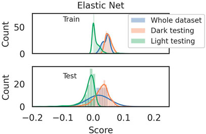
FIGURE 6. Train and test score for Elastic Net on the three dataset splits. Both quantities for the three splits are very low.

FIGURE 7. Train and test score for Random Forest. The train score is good, while the test score shows high variability, being acceptable most of the time but falling to negative values sometimes.
The performances of the two models are very different: looking at train and test scores for the eNet, we see that the model cannot describe this dataset. A score close to zero indicates that we cannot do better than random guessing, which indicates the model’s complete inability to capture patterns in the data (we non-etheless show the results in the Supplementary Figures S7–S9). On the other hand, RF performs better than eNet and can better describe the data. The test score is much lower than the train score, indicating poor generalization capabilities. Still, the performance is acceptable for such a complicated task, at least with the available data and all the data quality issues we discussed. The significant difference in performance between eNet and RF lets us conclude that a non-linear model, such as RF and Gradient Boosting, can satisfactorily model the dataset. A linear model, even an advanced one like eNet, cannot capture the patterns in the data that relate the device properties to its stability.
Figure 8 shows the 20 most important features that the RF model identified for the complete dataset while also showing the importance of such features for the other two dataset splits. RF model captured many features known to influence the thermal, moisture, or photo-stability of perovskite solar cells. The magnitudes of stresses (temperature, relative humidity) applied are predictably among the top influencing factors. And so is the perovskite composition, particularly the presence of MA or FA organic species as a monovalent cation or iodine as anion will generally result in less resilient perovskite materials. Multiple transport materials investigated as options for electron or hole transport layers significantly influence the device stability, and RF predictions agree on this point too. See an extended list of features and their impacts on stability in Supplementary Figures S4–S6.

FIGURE 8. Feature importance for the Random Forest model. The different colors identify the possible dataset splits. We show the 20 most important features when modeling the complete dataset.
Some predictions are less straightforward to verify, such as the significance of solvents, quenching, and annealing procedures. Though they influence perovskite crystallization and, therefore, device stability, it is hard to tell at the moment whether their role is as defining for the final device stability as predicted by the RF results. While it is interesting to investigate these factors’ importance on the PSC stability experimentally, we believe we need to improve our data-driven predictions to provide confident guidance for the experimental research.
Splitting the dataset into light and dark testing conditions while removing performance-related features shows that different features are selected as the most important. This is in accordance with different degradation mechanisms present with and without illumination. Given the low performance of the models, the numbers come with high uncertainty. However, we believe it is a good starting point for demonstrating the potential of ML methods to dramatically accelerate the learning process with a reduced number of (extremely time-consuming!) aging experiments.
As previously mentioned, we ran the learning curves experiments in three different settings. In the first setting, we use the database in its original form to check how good the power law approximation for the learning process is. As shown in Figure 9, the approximation seems appropriate, hence we extrapolate the learning curves to a dataset size of 10,000 data points to simulate the performance we could obtain when more data is added to the database. The second and third settings simulate an increase in data quality in two different ways: dropping noisy features and dropping noisy data points. By noisy, we mean features and data points with the highest number of missing values. If we consider the tabular representation of data that is usually adopted when applying machine learning to this type of data, in the first case, we are dropping columns, while in the second, we are dropping rows.
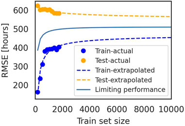
FIGURE 9. Learning curves as derived for the complete dataset. Extrapolation to size 10,000 of the train set.
Figure 9 shows the interpolation points for computing the learning curves and the extrapolation to a larger train set size when modeling the complete dataset. The limiting performance represents the average between train and test errors at each train set size. This experiment shows that the performance we can obtain from a much larger dataset than the one used in this study (10,000 points compared to the current 1,800) is not much better in terms of the test error. The performance looks already saturated and adding more data with the same quality and statistical properties is not expected to improve the model’s performance.
In this second experiment, we simulate higher-quality datasets by iteratively removing noisy features from the training set according to the number of missing values they contain. We remove the feature with the most missing values and then the less noisy ones, one at a time. We define the baseline performance of the ML model as the value of the test error extrapolated to 10,000 when using the complete train set, with no features removed. This baseline performance will also be used in the following experiment, where we remove noisy data points. Figure 10A shows the percentage change in extrapolated root mean squared error (RMSE) for each dataset compared to the baseline performance. It is clear from the figure that the extrapolated performance does not significantly change when removing noisy features. This might indicate that the benefit of having fewer missing values is canceled out by having less information about the devices, compared to when the parameters are reported.
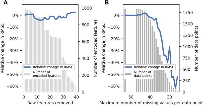
FIGURE 10. (A) Relative change in the extrapolated test RMSE when removing noisy features (the abscissa indicates the number of raw features removed from the 67 initial features; each raw feature might correspond to multiple encoded features). The baseline is taken as the extrapolated RMSE computed on the complete dataset. The grey bars indicate how many encoded features are left in the dataset after removing the noisy ones. (B) Percent change in the extrapolated test RMSE when removing noisy data points. The baseline is taken as the extrapolated RMSE computed on the complete dataset. The grey bars indicate how many data points are left in the dataset after removing the noisy ones.
The third experiment simulates higher-quality datasets by iteratively removing noisy data points, i.e., data points with a higher number of missing values (or devices with the least reported information). We remove the noisiest data points and then remove points with a lower noise level. Figure 10B shows the percentage change in extrapolated RMSE for each dataset compared to the baseline performance. The bars in the figure represent the number of data points left after removing the noisy ones, while the horizontal axis shows the maximum number of missing data values allowed for each dataset.
In contrast with the previous experiment, we observed pronounced improvement in the test score with higher quality data. However, we have to treat these results carefully. Removing data points lowers the statistical significance of the results and might also make the learning task easier, improving performance. Nevertheless, the trend is evident even for a reasonably sized dataset, around 1,000 data points, that are still larger than all similar datasets used in the literature.
Better conclusions can be drawn by comparing what happens when we remove features or data points: the first scenario corresponds to considering fewer properties of a device for an ML task, and the second corresponds to having only entries with a given quality in terms of the number of missing values. The difference in the evolution of the expected performance suggests how the features are relevant, and we need to collect them if we want to significantly improve the performance of machine learning models used for applications similar to the one explored in this study.
Machine learning techniques are optimized to predict a target variable; in our case, the lifetime is defined as T80. In this last section, we want to discuss how representative this metric is for describing perovskite solar cell stability. In the context of projects involving “Big Data,” the large number of aging curves available demands the programmatic extraction of stability metrics, which requires exact definitions, contrary to manually extracting FOMs from the aging curves. We have programmatically extracted different stability FOMs for PSCs, defined above, and compared them pairwise to assess their agreement. For this, we used the in-house data set with complete time series for aging experiments available. Figure 11 shows how T80 correlates to four other FOMs; the actual value of the Pearson correlation coefficient is shown on the upper edge of every sub-figure.
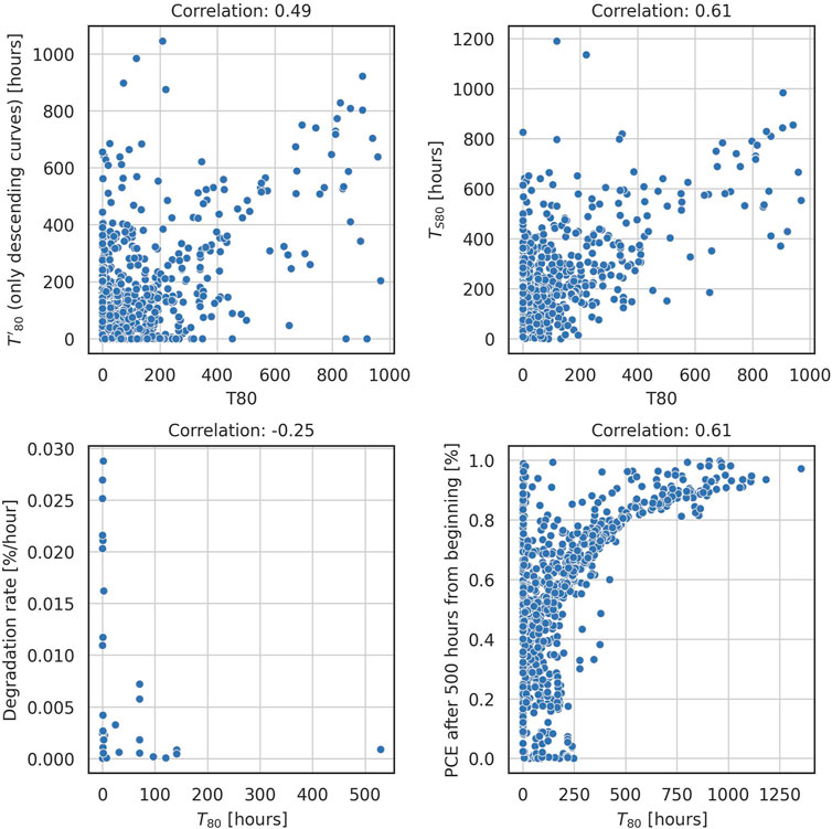
FIGURE 11. Scatter plot of T80 against four other stability figures of merit. Above every plot, the corresponding Pearson correlation coefficient is shown.
Figure 12 focuses only on examining the normalized PCE after a given time has passed during the experiment. We have compared the PCE value after 100 h of aging against those after 250, 500, and 1,000 h following the suggestion that it might be possible to reasonably extrapolate shorter aging experiments (Almora et al., 2021).

FIGURE 12. Scatter plot and correlation of the PCE normalized with the PCE at time 0, after 100 h, and the PCE at 250, 500, and 1,000 h.
From Figures 11, 12, it is clear how even FOMs with very similar definitions can result in very different values for PSCs aging curves. More importantly, they do not always agree regarding which devices are more stable. This is due to the wide variety of PSCs’ aging behaviors, which makes identifying a universal FOM for stability a non-trivial task. An agreement on the FOM to use that best describes what we mean by stability of PSCs will surely help in improving the performance of ML models. The low correlation between FOMs shows that the single number fed to ML algorithms might not represent the task we are trying to solve. This increases the difficulty of the task, which is already high due to other quality issues and the relatively small size of the available datasets compared to the number of parameters to consider.
Machine learning methods have a great potential to accelerate the development of more stable perovskite devices, potentially avoiding the extremely time-consuming aging experiments. Using the perovskite database project that summarizes available literature, we have demonstrated the possibility of applying ML for PSC stability data, although only non-linear methods (such as random forest) show promising results. Even in this case, however, data quality remains a significant challenge. Learning curves experiments indicate that just increasing the amount of data (i.e., collecting more aging experiments) has a limited positive effect on boosting the confidence of ML forecast. Instead, we show that it is critical to improve the data quality by reporting as complete information on the device manufacturing and aging conditions as possible. More accurate data leads to higher statistical relevance of the results, better ability of the ML algorithms to capture patterns in the data, and increased prediction performance.
Another, perhaps more significant, challenge is defining the FOMs for stability used as target variables for the ML analysis. With in-house data, we show that the variety of behaviors observed in the aging curves of perovskite devices leads to the dependence of the results on the choice of the metric. A single number (e.g., T80) cannot capture the complexity of such curves and, therefore, is unlikely to be an optimal choice. Sharing the complete aging curves would be vital to solving this problem. These shared data would facilitate the discussion on universal FOMs that describe stability for perovskite solar devices in a meaningful and precise way.
We encourage perovskite researchers to report more complete data regarding the experiments and full aging curves since we believe this can significantly accelerate the development of commercially viable perovskite solar devices through machine learning.
The original contributions presented in the study are included in the article/Supplementary Material, further inquiries can be directed to the corresponding author.
PG has performed the data preparation and machine learning analysis. PG and MK wrote the first draft of the manuscript. HK, NH, and AA provided the in-house database of aging experiments. PG, MK, HK, EU, TJ, and CU contributed to the conception of the study. MK, RS, and CU contributed to the supervision of the project. All authors contributed to the manuscript revision.
PG acknowledges the support of the Helmholtz Einstein International Berlin Research School in Data Science (HEIBRiDS). MK, RS, and CU acknowledge the support of the European partnering project TAPAS (PIE-0015). HK acknowledges the support from the HyPerCells graduate school. HK acknowledges the VIPERLAB project funded by the European Union’s Horizon 2020 research and innovation programme under grant agreement N°101006715
The authors declare that the research was conducted in the absence of any commercial or financial relationships that could be construed as a potential conflict of interest.
All claims expressed in this article are solely those of the authors and do not necessarily represent those of their affiliated organizations, or those of the publisher, the editors and the reviewers. Any product that may be evaluated in this article, or claim that may be made by its manufacturer, is not guaranteed or endorsed by the publisher.
The Supplementary Material for this article can be found online at: https://www.frontiersin.org/articles/10.3389/fenrg.2023.1118654/full#supplementary-material
Almora, O., Baran, D., Bazan, G. C., Berger, C., Cabrera, C. I., Catchpole, K. R., et al. (2021). Device performance of emerging photovoltaic materials (version 2). Adv. Energy Mater. 11 (48), 2102526. doi:10.1002/aenm.202102526
Best Research-Cell Efficiency Chart, (2023). Best research-cell efficiency Chart’. n.d. https://www.nrel.gov/pv/cell-efficiency.html (Accessed February 17 2023).
Brinkmann, K. O., Gahlmann, T., and Riedl, T. (2020). Atomic layer deposition of functional layers in planar perovskite solar cells. Sol. RRL 4 (1), 1900332. doi:10.1002/solr.201900332
Chen, J., Feng, M., Zha, C., Shao, C., Zhang, L., and Wang, L. (2022). Machine learning-driven design of promising perovskites for photovoltaic applications: A review. Surfaces Interfaces 35 (December), 102470. doi:10.1016/j.surfin.2022.102470
Chen, M., Ju, M. G., Garces, H. F., Carl, A. D., Ono, L. K., Hawash, Z., et al. (2019). Highly stable and efficient all-inorganic lead-free perovskite solar cells with native-oxide passivation. Nat. Commun. 10 (1), 16. doi:10.1038/s41467-018-07951-y
Chi, W., and Banerjee, S. K. (2021). Stability improvement of perovskite solar cells by compositional and interfacial engineering. Chem. Mater. 33 (5), 1540–1570. doi:10.1021/acs.chemmater.0c04931
Cortes, C., Jackel, L. D., Solla, S. A., Vapnik, V., and Denker, J. S. (1993). Learning curves. Asymptot. Values Rate Convergence’ 6 (November), 327–334.
David, T. W., Helder Anizelli, T., Jacobsson, T. J., Gray, C., Teahan, W., Kettle, J., et al. (2020). Enhancing the stability of organic photovoltaics through machine learning. Nano Energy 78 (December), 105342. doi:10.1016/j.nanoen.2020.105342
Dipta, S. S., and Uddin, A. (2021). Stability issues of perovskite solar cells: A critical review. Energy Technol. 9 (11), 2100560. doi:10.1002/ente.202100560
Foo, G. S., Polo-Garzon, F., Fung, V., Jiang, D., Overbury, S. H., and Wu, Z. (2017). Acid–base reactivity of perovskite catalysts probed via conversion of 2-propanol over titanates and zirconates. ACS Catal. 7 (7), 4423–4434. doi:10.1021/acscatal.7b00783
Green, M. A., Dunlop, E. D., Hohl-Ebinger, J., Yoshita, M., Kopidakis, N., Bothe, K., et al. (2022). Solar cell efficiency tables (version 60). Prog. Photovoltaics Res. Appl. 30 (7), 687–701. doi:10.1002/pip.3595
Jacobsson, T. J., Adam, H., García-Fernández, A., Anand, A., Al-Ashouri, A., Anders, H., et al. (2022). An open-access database and analysis tool for perovskite solar cells based on the FAIR data principles. Nat. Energy 7 (1), 107–115. doi:10.1038/s41560-021-00941-3
James, G., Witten, D., Hastie, T., and Tibshirani, R. (2013). An introduction to statistical learning, 103. New York, NY: Springer Texts in Statistics. doi:10.1007/978-1-4614-7138-7Springer New York
Khenkin, M. V., Katz, E. A., Abate, A., Brabec, C., Abate, A., Bardizza, G., et al. (2020). Consensus statement for stability assessment and reporting for perovskite photovoltaics based on ISOS procedures. Nat. Energy 5 (1), 35–49. doi:10.1038/s41560-019-0529-5
Köbler, H., Neubert, S., Jankovec, M., Glažar, B., Haase, M., Hilbert, C., et al. (2022). High-throughput aging system for parallel maximum power point tracking of perovskite solar cells. Energy Technol. 10 (6), 2200234. doi:10.1002/ente.202200234
Liu, Y., Yan, W., Han, S., Zhu, H., Tu, Y., Guan, L., et al. (2022). How machine learning predicts and explains the performance of perovskite solar cells. Sol. RRL 6 (6), 2101100. doi:10.1002/solr.202101100
Lu, Q., Yang, Z., Meng, X., Yue, Y., Ahmad, M. A., Zhang, W., et al. (2021). A review on encapsulation technology from organic light emitting diodes to organic and perovskite solar cells. Adv. Funct. Mater. 31 (23), 2100151. doi:10.1002/adfm.202100151
Mazumdar, S., Zhao, Y., and Zhang, X. (2021). Stability of perovskite solar cells: Degradation mechanisms and remedies. Front. Electron. 2. doi:10.3389/felec.2021.712785
Myung, C. W., Hajibabaei, A., Cha, J., Ha, M., Kim, J., and Kwang, S. (2022). Challenges, opportunities, and prospects in metal halide perovskites from theoretical and machine learning perspectives. Adv. Energy Mater. 12 (45), 2202279. doi:10.1002/aenm.202202279
Nath, B., Ramamurthy, P. C., Mahapatra, D. R., and Hegde, G. (2022). Electrode transport layer–metal electrode interface morphology tailoring for enhancing the performance of perovskite solar cells. ACS Appl. Electron. Mater. 4 (2), 689–697. doi:10.1021/acsaelm.1c01100
Odabasi, C., and Yildirim, R. (2020). Machine learning analysis on stability of perovskite solar cells. Sol. ENERGY Mater. Sol. CELLS 205 (February). doi:10.1016/j.solmat.2019.110284
Roesch, R., Faber, T., von Hauff, E., Thomas, M., Brown, M., Hoppe, H., et al. (2015). Procedures and practices for evaluating thin-film solar cell stability. Adv. Energy Mater. 5 (20), 1501407. doi:10.1002/aenm.201501407
Seung, H. S., Sompolinsky, H., and Tishby, N. (1992). Statistical mechanics of learning from examples. Phys. Rev. A 45 (8), 6056–6091. doi:10.1103/PhysRevA.45.6056
Tiihonen, A., Miettunen, K., Halme, J., Lepikko, S., Poskela, A., and Peter, D. (2018). Critical analysis on the quality of stability studies of perovskite and dye solar cells. Energy and Environ. Sci. 11 (4), 730–738. doi:10.1039/C7EE02670F
Yılmaz, B., and Yıldırım, R. (2021). Critical review of machine learning applications in perovskite solar research. Nano Energy 80, 105546. doi:10.1016/j.nanoen.2020.105546
Keywords: perovskite solar cell, stability, machine learning, figures of merit, learning curves, database, feature importance analysis, halide perovskite
Citation: Graniero P, Khenkin M, Köbler H, Hartono NTP, Schlatmann R, Abate A, Unger E, Jacobsson TJ and Ulbrich C (2023) The challenge of studying perovskite solar cells’ stability with machine learning. Front. Energy Res. 11:1118654. doi: 10.3389/fenrg.2023.1118654
Received: 07 December 2022; Accepted: 21 March 2023;
Published: 03 April 2023.
Edited by:
Wilfried G. J. H. M. Van Sark, Utrecht University, NetherlandsReviewed by:
Terry Chien-Jen Yang, University of Cambridge, United KingdomCopyright © 2023 Graniero, Khenkin, Köbler, Hartono, Schlatmann, Abate, Unger, Jacobsson and Ulbrich. This is an open-access article distributed under the terms of the Creative Commons Attribution License (CC BY). The use, distribution or reproduction in other forums is permitted, provided the original author(s) and the copyright owner(s) are credited and that the original publication in this journal is cited, in accordance with accepted academic practice. No use, distribution or reproduction is permitted which does not comply with these terms.
*Correspondence: Mark Khenkin, bWFyay5raGVua2luQGhlbG1ob2x0ei1iZXJsaW4uZGU=
Disclaimer: All claims expressed in this article are solely those of the authors and do not necessarily represent those of their affiliated organizations, or those of the publisher, the editors and the reviewers. Any product that may be evaluated in this article or claim that may be made by its manufacturer is not guaranteed or endorsed by the publisher.
Research integrity at Frontiers
Learn more about the work of our research integrity team to safeguard the quality of each article we publish.