 Dorian Esteban Guzman Razo
 Henrik Madsen2
94% of researchers rate our articles as excellent or good
Learn more about the work of our research integrity team to safeguard the quality of each article we publish.
Find out more
METHODS article
Front. Energy Res., 01 June 2023
Sec. Solar Energy
Volume 11 - 2023 | https://doi.org/10.3389/fenrg.2023.1060215
This article is part of the Research TopicRising Stars in Energy Research: 2022View all 10 articles
Accurately predicting and balancing energy generation and consumption are crucial for grid operators and asset managers in a market where renewable energy is increasing. To speed up the process, these predictions should ideally be performed based only on on-site measured data and data available within the monitoring platforms, data which are scarce for small- and medium-scale PV systems. In this study, we propose an algorithm that can now-cast the power output of a photovoltaic (PV) system with high accuracy. Additionally, it offers physical information related to the configuration of such a PV system. We adapted a genetic algorithm-based optimization approach to parametrize a digital twin of unknown PV systems, using only on-site measured PV power and irradiance in the plane of array. We compared several training datasets under various sky conditions. A mean deviation of −1.14 W/kWp and a mean absolute percentage deviation of 1.81% were obtained when we analyzed the accuracy of the PV power now-casting for the year 2020 of the 16 unknown PV systems used for this analysis. This level of accuracy is significant for ensuring the efficient now-casting and operation of PV assets.
Photovoltaic (PV) system installed capacity has doubled globally in the past 3 years, hitting a terawatt in April 2022, and is projected to reach 2.3 TW by 2025 (SolarPower Europe, 2022). The surge in PV capacity is being driven by a variety of factors, including favorable laws and growing public knowledge of solar energy’s advantages, which are causing this remarkable increase. According to predictions by the International Energy Agency (IEA) in 2022, PV electricity will generate an extra 180 TW-hours by 2030, making up 60% of all renewable energy production (International Energy Agency, 2022). An additional important factor contributing to the success of PV systems is their rapidly declining cost. The average global weighted levelized cost of electricity (LCOE) for the utility-scale PV has dropped by 13% per year since 2010, reaching around 4.8 cents per kilowatt-hour in 2021 (IRENA, 2021). This trend is expected to continue as technology improves and economies of scale are reached, making solar energy an increasingly attractive and cost-effective option for energy generation.
Simulating and forecasting the PV power output of a utility-scale PV plant is very important for both plant managers and electricity network operators. Indeed, an accurate PV yield study is one of the most crucial elements for a successful bankability and feasible study of a PV power plant (Müller et al, 2016). Reliable irradiance data and an effective PV power simulation tool are crucial for correctly forecasting the power output of a PV system. Although the irradiance data should be approximated with high accuracy and temporal resolution, the simulation tool should mimic the behavior of a PV system under various weather and operating conditions. These two elements can be used to produce an accurate and reliable PV yield study (Müller et al, 2007). Achieving an accurate PV power simulation often requires specific physical and technical data for the PV system or subsystem being modeled, according to Müller et al (2007. Yet, these data are not always available or may be incomplete for certain PV systems or subsystems in a larger PV portfolio. As a result, accurate power prediction for such systems may be challenging. Moreover, irradiance data used for PV power simulation can be derived from satellite observations or measured on-site. However, inconsistencies between the on-site and satellite-derived irradiance data can propagate proportionally up to the simulated PV power output. Furthermore, inaccuracies in the different models used within the PV power modeling process can amplify these errors (Urraca et al, 2018a).
As suggested in IEC 61850-7-420 (IEC, 2009), PV systems are expected to have basic meteorological measurement devices for ambient temperature and solar irradiation. Considering this, our work focuses on developing an optimization algorithm that learns the basic parameters of an unknown small- or medium-scale PV system or subsystem. Thereby, an accurate PV power simulation is implemented based on only the on-site measured PV power and on-site measured meteorological data.
This work is a continuation of a previous publication (Guzman Razo et al, 2020), in which we used a genetic algorithm (GA) approach to parametrize and create a digital twin of an unknown PV system based on the measured PV power and data provided by SolarGIS s.r.o., including air temperature and satellite-derived irradiation. Next, we created a digital twin and accurately simulated the behavior of that specific PV power plant under different outdoor conditions. This publication will be referred to as Guzman1 in the following sections of this work.
GA optimization offers a deterministic and time-efficient alternative for curve fitting. Additionally, GA optimization characteristically offers an alternative (crossover and mutation) to avoid solving for local minima. In contrast with Guzman1, in this work, we created a digital twin of an unknown small- or medium-scale PV system without exogenous information. In other words, the current GA optimization approach is based on only the on-site measured PV power and on-site measured meteorological data, specifically, module temperature (
This work aims to
• Show an accurate method to create a digital twin of a PV system based on the GA optimization;
• Learn and optimize basic parameters of an unknown PV system or subsystem without the need for external data, including the PV module temperature coefficient, Heydenreich a, b, and c, DC-to-AC ratio, and nominal power;
• Evaluate the accuracy of the digital twin created with different lengths of training data;
• Evaluate the now-cast precision of a digital twin trained with either all-sky or clear-sky conditions;
• Propose potential accuracy improvement for the GA optimization approach proposed in this study.
This article is structured as follows: We present a summary of previous publications for PV simulation and forecasting using exclusively monitoring data and metrics to evaluate the results (Section 2). In Section 3, we show how we adapted the methodology from Guzman1 and present a description of the data to be used within this study. In Section 4, we offer a discussion regarding the results of the GA optimization, namely, digital twin parameters and the now-casting results using these parameters. In addition, we validate the methodology proposed in the current study and propose an example to improve the now-casting accuracy considering additional weather information. Finally, in Section 5, we present the main conclusion of this work and future improvements.
Short-term PV power forecasting is key for achieving a balance between energy consumption and production in a grid with high PV penetration, applications for storage management, and reliability of the bidding markets. This work focuses on creating an accurate tool that can be applied for PV parameter extraction and short-term PV power forecasting.
In this section, we present methods suggested in the literature to create a model of a PV system and the use of that model for short-term forecasting with no additional data to those collected on-site by the data acquisition systems. Moreover, in this section, we show the accuracy metrics used to evaluate the method proposed in this publication.
At present, several machine-learning approaches have been studied to develop models for PV power forecasting. These models use on-site power-measured data in combination with numerical weather prediction or satellite-derived data. These methods commonly minimize data used while increasing the overall accuracy of the solution. However, these approaches rarely provide a physical description of the PV system’s components and configuration. In this study, we focus on methods without exogenous data, in other words, methods that include exclusively on-site PV power-measured data and on-site measured weather data.
Mandal et al (2012) offered a solution with a mix of wavelet transform (WT) and different machine learning techniques. A PV system model is created by dividing the PV power time-series data between the ill-mode and non-linear fluctuations (spikes in power). After that, four components are extracted by downsampling and then filtered using low-pass filters. Finally, the PV system model is obtained after a wavelet reconstruction, including some upsampling after feeding each one of the individual components from the TW into different neural networks. A mean absolute percentage deviation (MAPD) of 2.38% can be achieved for clear-sky periods of PV power forecasting. This method has a horizon of 12 h, and its performance decreases considerably when cloudy or rainy days are forecasted (Mandal et al, 2012).
Almeida et al (2015) proposed an alternative model for PV power output forecasting that includes on-site weather data. They applied a random forest (RF) model to create a PV model and then used numerical weather prediction data to forecast the PV power output. The results suggested an MAPD of 9.5% between the forecasted and the on-site measured data (Almeida et al, 2015).
This contribution proposed a data-driven approach based on the use of artificial neural networks (ANNs) trained with measured PV power to create day-ahead forecasts of PV power. Unlike other methods, this solution does not require any weather data and offers an MAPD of 6.64% for the best-case scenario.
The suggestions from González Ordiano et al (2017) on using weather-free approaches based on machine learning techniques are particularly relevant. This contribution proposed a data-driven approach based on the use of ANNs trained with measured PV power to create day-ahead forecasts of PV power. Unlike other methods, this solution does not require any weather data and offers an MAPD of 6.64%, for the best-case scenario (González Ordiano et al, 2017).
In contrast to the various machine learning solutions, there are only a few physics-based or hybrid methods in the literature that provide a description of a specific PV system or subsystem’s configuration.
The article by Ogliari et al (2017) presents a model for next-day PV power forecasting based on the well-known single-diode model, which can consider either three or five parameters. In addition, the authors propose two other approaches, an ANN model and a hybrid model combining both physical and ANN models, for next-day forecasting. The ANN and hybrid models use historical weather data for training, with two different training approaches. However, it is important to note that the physical parameters required for the single-diode model need to be determined from the PV module’s datasheet or from previous experiments (Ogliari et al, 2017).
It is important to mention that the physical model used in Ogliari et al can only describe the behavior of a PV module under outdoor conditions without considering the losses from the rest of the components of a PV system or subsystem, i.e., cabling losses and inverter efficiency (DC-to-AC ratio). Ogliari et al reported achieving mean absolute deviations (MADs) of 19.1 W and 20.2 W for the three- and five-parameter physical models, respectively. In the case of the hybrid method, the MAD is 12.46 W for the best case of the first training approach and 12.5 W for the best case of the second training approach.
Similar to Guzman1, we used four values to evaluate the accuracy of the digital twin created by the GA optimization method offered here, i.e., root mean square deviation (RMSD), MAPD, mean bias deviation (MBD), and MAD. Eqs. 1–4, respectively, show how we calculate the values.
where
In this work, we adapted some steps of a PV power simulation tool developed in-house by Fraunhofer ISE and suggested by Dirnberger et al (2015) and Müller et al (2016). We optimized the parameters required by the PV system simulation tool using the GA and created a digital twin of an unknown PV system or subsystem.
Figure 1 shows the overall methodology used to parameterize an unknown PV system or subsystem, with the GA optimization process, the PV system simulation tool (and its main models), the inputs (i.e., initial parameters, and on-site measured meteorological and PV power), and the optimized parameters as an output, which are later used as a digital twin. The green dotted rectangle represents the GA optimization process, while the orange dotted rectangle represents the PV system simulation process and its corresponding steps.
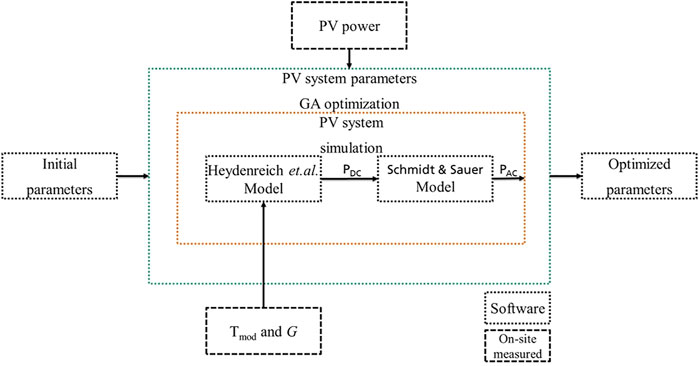
FIGURE 1. Interaction between inputs and outputs of the overall GA optimization methodology.
As shown in the orange rectangle in Figure 1, the adapted PV system simulation tool can simulate AC PV power with only on-site measured
Using equations suggested by Heydenreich et al (2008)(Eqs. 5, 6), we simulated DC PV power (Heydenreich et al, 2008). First, the DC PV power at a temperature of 25°C, or standard test conditions (STCs) Eq. 5, was simulated, and later, we translated that simulated DC PV power to the on-site measured temperature and irradiance conditions Eq. 6.
where
where
To simulate AC PV power output, we used the inverter model proposed by Schmidt and Sauer (1994), accounting for 1% of cabling losses (Schmidt and Sauer, 1994).
To define the best climatic conditions for the parameter extraction, in the GA optimization training phase, we created two different training sets:
• The first set includes all possible conditions measured on-site i.e., overcast and clear-sky-like moments. This training dataset will be referred to in this work as all-sky.
• The second set filters out the overcast moments and only includes clear-sky-like moments. This training dataset will be referred to in this work as clear-sky.
We detected and filtered clear-sky-like moments based on the two-step process described in detail in Guzman1. First, based on the on-site measured PV power data, a statistical clear-sky curve was created following the method implemented and proposed by Stein et al (2012) and Reno and Hansen (2016). Next, with the “detect_clearsky” function from the PVLib library (Holmgren et al, 2020), we detected clear-sky-like moments. Training datasets of both clear-sky and all-sky moments comprised only on-site measured PV power data and their correspondent on-site measured
In general terms, we based our GA algorithm on the technique proposed by Holland (1975). Although GA optimization is considered a traditional optimization algorithm, it has been rarely implemented in the solar industry. Moreover, inherently, the GA optimization offers an accurate and time-efficient deterministic approximation of the real parameters of unknown PV systems and subsystems. Additionally, the GA performs effectively for problems relating to dynamic environments where an optimal answer can evolve over time. In these situations, the solution space might be too big to thoroughly explore, and the ideal answer can change as the situation changes (Mori and Kita, 2000).
The novelty of this work relies on the fact that we can extract the main characteristics of an unknown PV system or subsystem by implementing a similar GA optimization to the one proposed by Holland (1975) within a stepwise process. In this work, we opted for a stepwise optimization process to reduce the compensation between parameters.
To extract the most accurate PV system parameters, we minimized the MAD (see Eq. 4) between simulated AC PV power and on-site measured AC PV power. The MAD of the best member of the population and population mean MAD are two key performance indexes to monitor throughout the GA optimization. The optimization process is interrupted if neither of the two performance indexes improves any more. A detailed description of this process can be found in Guzman1.
In the GA optimization, to create the initial population of PV system parameters to be evaluated and optimized, we began by defining the initial parameters for this work as 1-kilowatt peak (kWp) for nominal power, −0.43 %/°C for the power temperature coefficient, and a ratio of 1 for the DC to AC power.
Next, we normalized the on-site measured AC PV power by the maximum measured value. By normalizing on-site measured AC PV power, we compared it with the simulated AC PV power of a 1-kWp installed capacity system. It is important to mention that the measured
• With cross-validation optimization, we selected the best set of a, b, and c parameters for (Eq. 5). The cross-validation optimization process was based on a database comprising 107 sets of three parameters, described in Guzman1, including the results from Fraunhofer ISE CalLab efficiency measurements of 107 PV modules at different irradiance levels. We simulated DC PV power, using each one of the 107 sets of parameters, and compared it with the normalized AC power. We considered the lower MAD as the optimum set of parameters for the simulated PV system.
• We used GA optimization to learn the PV module temperature coefficient by minimizing the MAD between simulated DC PV power resulting from Eq. 6) and normalized-measured AC PV power.
• To optimize the DC-to-AC ratio, we used GA optimization to minimize the MAD between simulated AC PV power (based only on the efficiency section of the Schmidt and Sauer model) and normalized-measured AC PV power.
• Finally, we used GA optimization to minimize the MAD between simulated AC PV power and measured AC PV power (non-normalized) to extract the PV system nominal power.
The results obtained from applying the PV models with the optimized parameters in this study accurately reflect the real behavior of the tested PV system. As a result, by using these optimized parameters, we can create a digital twin of the PV system or subsystem and simulate its performance by changing the irradiance and temperature conditions to current (now-cast) or future (forecast) values.
Figure 2 shows two digital twins created from on-site measurements of a system located in southwest Germany with a training dataset of 30 days length (before the day to be tested), in which all-sky conditions are considered. On the left-hand side, subplot (a) shows a PV power simulation for a clear-sky-like day: measured PV power, the measured
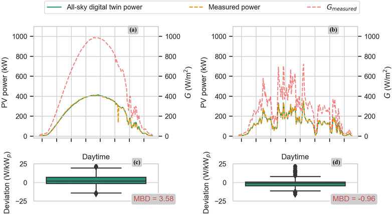
FIGURE 2. Two-day results of a digital twin from a system located in southwest Germany. In subfigure (A, B), the red dotted line shows the irradiance G measured on-site, the orange dotted line shows the AC PV powermeasured on-site, and the solid green line shows the AC PV power forecasted by the digital twin parametrized with a 30-days long data set considering all-sky conditions. Subfigures (C, D) show the deviation betweenthe AC PV power measured on-site and the AC PV power forecasted. The left side of FIGURE 2 shows a clear-sky like day and the right side shows an overcast-like day.
In this work, we used a database comprising 16 real on-site measured PV systems installed in Germany, which are part of the Fraunhofer ISE monitoring portfolio. The geographical location of those systems can be observed in Figure 3.
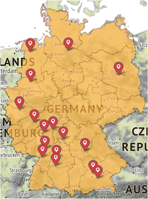
FIGURE 3. Location of the 16 real on-site measured PV systems.
The database used here, collected between 2018 and 2020, consists of a time series of approximately 567,500 points of 5-min resolution including three main features: measured PV power, measured

TABLE 1. Nominal power and
Additionally in Section 4.3.1, we used daily observations of snow depth data from the Deutscher Wetterdienst (German Weather Service) climate data center (CDC) (Kaspar et al, 2013) for the year 2020, for all 16 locations.
In the first part of this section, our goal was to demonstrate the impact of different lengths of training datasets on the parametrization and now-casting performance of the digital twin. We analyzed data from a PV system located in southwest Germany (ID 5) to investigate this effect. The selection of PV system ID 5 was arbitrary and was chosen out of the 16 real PV systems in our database to randomize the process and prioritize our research on the effect of different training dataset lengths on PV system parametrization.
The reported design parameters from the PV system ID 5 are the following:
• Temperature coefficient (%/°C): -0.43
• Heydenreich a: 0.001084
• Heydenreich b: -7.247061
• Heydenreich c: -156.5457
• DC-to-AC ratio: 1.04
• Nominal power (kWp): 553
• Year of construction: 2010
Next, we evaluated the rest of the PV systems within the database using the best-performing length for training the digital twin. Additionally, we investigated the potential for improving now-casting accuracy by considering locally measured snow deposition information. Finally, we discuss limitations and possible future improvements at the end of this section.
To evaluate the effect of seasonality and the length of training data on the parametrization of the digital twin and the accuracy of now-casting, we randomly selected 1 day per week of the year 2020 (a total of 52 days). For each selected day, we used six different training dataset lengths, including 30, 60, 90, 120, 150, and 182 days prior to the selected day. We also identified clear-sky conditions within all the training datasets and trained the GA using both all-sky and clear-sky moments. Each combination of training dataset length, selected day, and all/clear-sky moments resulted in a different set of parameters (digital twin) for the PV system under consideration.
Figure 4 shows plots of optimization results for nominal power and the DC-to-AC ratio, considering 52 randomly chosen days and different training set lengths: 30, 60, 90, 120, 150, and 182°days. Optimization results for the temperature coefficient have been reported constantly throughout the 52°days (−0.4%/°C) and, therefore, are not shown in the figure. In general, while considering all-sky moments, the DC-to-AC ratio (see subplot c)) remains more constant than while considering only clear-sky moments. In contrast to that, optimization for nominal power remains more stable while considering only clear-sky moments (see subplot b)).
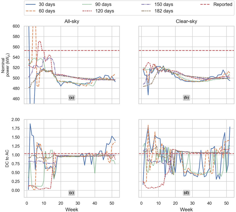
FIGURE 4. GA optimization results for nominal power and the DC-to-AC ratio. A total of 52 days were chosen, of the year 2020 considering six different training datasets for each day; all-sky and clear-sky conditions with 30, 60, 90, 120, 150, and 182°days of training datasets. The 30-day dataset is represented by the solid blue line, 60-day dataset is represented by the orange dashed-line, 90-day dataset is represented by a green dotted line, 120-day dataset is represented by the dotted–dashed red line, 150-day dataset is represented by the dotted–dashed blue line, 182-day dataset is represented by the dotted–dashed brown line, and the reported parameter is represented by a horizontal red dashed-line. Figure 4 is divided into left-hand (A, C) and right-hand (B, D) sections. The left-hand subplots (A, C) show optimized parameters for all-sky condition optimization, whereas the right-hand side subplots (B, D) show optimized parameters considering only clear-sky conditions.
The results of a quantitative analysis are included in Table 2. The analysis includes results from the GA optimization considering clear-sky and all-sky conditions for all the different training length datasets.
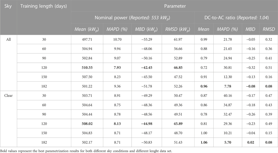
TABLE 2. Parametrization results of the GA optimization for PV system ID5 including all-sky and clear-sky conditions.
One of the advantages of parametrizing a PV system or subsystem based on only on-site measured data (including
The parametrization results for nominal power shown in Figure 4 are on the side of an underestimation. As mentioned previously, using only clear-sky moments seems to be more stable. As shown in Table 2, the best conditions for an accurate nominal power parametrization are as follows: all-sky conditions in combination with a 120-day training length. This combination shows a mean value of 510.55 kWp with an MAPD of only 7.93% and an MBD of only −42.45 kWp. In contrast to our previous publication (Guzman Razo et al, 2020), these values have reduced considerably from 10.69% and −84.24 kWp, respectively. This is most likely due to the increase in accuracy of
Given that the reported nominal power value is 553 kWp, there is still a deviation between it and the value extracted using the GA model. One possible explanation for this deviation could be attributed to a degradation rate, which according to Jordan et al (2016), is expected to be between 0.8% and 0.9% per year since the installation year (Jordan et al, 2016). For system ID5, which has been installed for 10 years to the date of the experimental data, a degradation rate of between 8% and 9% can be expected, resulting in a nominal power between 508.76 kWp and 503.23 kWp. The value calculated using the proposed GA model shows good agreement with the expected value. However, this should not be taken lightly as additional power losses can exist and require further investigation.
It seems that there is a trade-off between using all-sky conditions and clear-sky moments for parametrization of the AC-to-DC ratio; see Figure 4. Although all-sky conditions provide more stable results in a particular period, clear-sky moments tend to result in spreader results on the side of overestimation. However, regardless of the condition used, a training length of 182 days seems to be the most suitable for accurate parametrization; see Table 2. The best-case scenario shows a mean value of 1.06 with a 5.7% MAPD and an MBD of 0.02, which is an improvement from the MBD of −0.14 achieved in Guzman1.
As mentioned previously, a constant parameter has been estimated for the 52 test days for the power temperature coefficient. Therefore, the parametrization results of the Heydenreich et al model for PV system ID5, considering both scenario clear-sky and all-sky moments, are the following:
• Heydenreich a: 0.004326
• Heydenreich b: -11.275966
• Heydenreich c: -182.272483
Although the optimal conditions for parametrizing the presented model are defined based on clear-sky or all-sky conditions and the length of the training dataset, the accuracy of the now-casting must also be evaluated. For instance, if the nominal power is close to the reported value, it would receive a higher score. However, these values do not account for additional losses that are commonly present in PV systems under outdoor conditions, such as soiling and degradation.
Therefore, in the following subsection, we evaluated the accuracy of now-casting using the parameters calculated with different training dataset lengths.
To select the optimal training length for the GA algorithm presented here, in this section, we evaluate simulated PV power with parameters from the digital twin considering only daytime values. We randomly selected 52°days from the year 2020 of System ID 5 and generated a set of parameters for each of the 52°days in combination with different training lengths (30°days, 60°days, 90°days, 120°days, 150°days, and 182°days). Finally, we compared the simulated PV power with the on-site measured PV power.
To generalize and correlate the results offered here with any other PV system or subsystem, we measured the deviation in W/kWp installed. Table 3 shows the results of now-casting for all the training datasets (30, 60, 90, 120, 150, and 182°days) and all the conditions (all-sky and clear-sky).
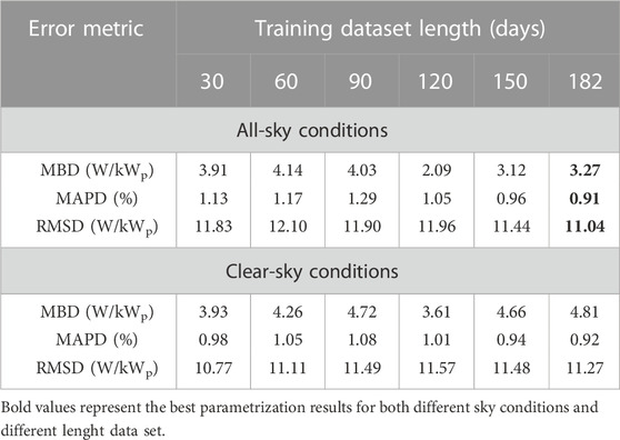
TABLE 3. Accuracy results of the digital twins created for 52 randomly chosen days in the year 2020. A total of 12 different training datasets including all-sky and clear-sky conditions with lengths of 30, 60, 90, 120, 150, and 182°days.
We evaluated the now-casting results based on the MAPD parameter. As shown in Table 3, the best combination of conditions and training length is achieved with all-sky conditions and a 182-day training dataset, resulting in an MAPD of 0.91%.
Figure 5 shows that the high variation in the parameterization, particularly in the DC-to-AC ratio, is not necessarily reflected in the now-casting results. The now-casting deviation using all-sky conditions (subfigure (a)) is consistently underestimated compared to the deviation using only clear-sky conditions (subfigure (b)), particularly for short training datasets (30–90°days). However, the absolute deviation of the now-casting is similar for both all-sky and clear-sky conditions, particularly for longer training data sets (120–182°days).
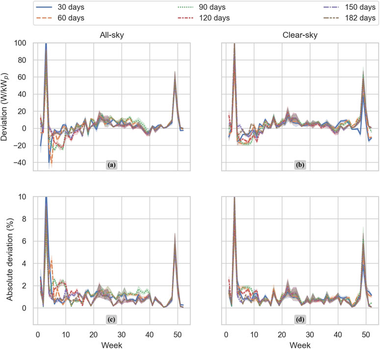
FIGURE 5. Digital twin now-casting results based on GA optimization. A total of 52 days chosen in the year 2020. Six different training datasets for each day were considered: All-sky and clear-sky conditions with 30, 60, and 90 days of training datasets. 95% confidence interval. The 30-day dataset is represented by the solid blue line, the 60-day dataset is represented by the orange dashed line, the 90-day dataset is represented by a green dotted line, the 120-day dataset is represented by the dotted–dashed red line, the 150-day dataset is represented by the dotted–dashed blue line, the 182-day dataset is represented by the dotted–dashed brown line, and the reported parameter is represented by a horizontal red dashed line. Figure 5 is divided into two vertical sections; on the left-hand side, we can see the results of the now-casting considering all-sky conditions (A, C), and the right-hand side, shows the results from the now-casting considering only clear-sky conditions (B, D).
Based on the results presented here, we considered that 182 days (or 6 months) based on all-sky conditions is the minimum required length to train GA optimization. With these condition-training lengths, it is possible to achieve an MBD of 3.27 kWp and an MAPE of only 0.91%. Previous publications, including Guzman1, reported an MAPE from 6% to 10% for now-casting tests (Ding et al, 2011; Mandal et al, 2012; Kaspar et al, 2013; Monteiro et al, 2013; Ibrahim et al, 2015; Landelius et al, 2019; Guzman Razo et al, 2020).
According to the results presented in the previous subsections, a training dataset length of 182°days is suggested to achieve high accuracy for both the digital twin parametrization and now-casting. To validate this suggestion, a 182-day training dataset was selected for each of the 16 monitored PV systems for the year 2020. Similar to the experiment described in the previous subsections, a random day from each week of the year 2020 was selected (52°days in total) to create a digital twin for each PV system on each selected day.
Figure 6 shows the PV power now-casting results for all 16 real PV systems. As observed, the mean deviation of all 16 real PV systems, in W/kWp installed, indicates an under-casting, −1.14, which is influenced by high-deviation peaks in winter, particularly for System ID15. Additionally, the figure shows that the MAD for all 16 real PV systems is merely 1.81%, indicating a good benchmark for short-term PV power forecasting.
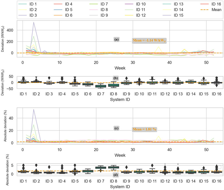
FIGURE 6. Deviation and absolute deviation of 52 days for now-casting for all the 16 real PV systems. In the upper section of the plot, subplots (A) and (B) show the deviation in W/kWp installed between the power now-casting and the power measured on-site. In the lower section of the plot, subplots (C) and (D) show the absolute deviation in percentage between the power now-casting and the power measured on-site. Subplots (A) and (C) show the distribution of the deviation per day and the mean value over all 16 PV systems. Subplots (B) and (D) show boxplots representing the distribution of the deviation per PV system, and high deviations are considered outliers and therefore ignored (see System ID 15, week 4).
In general terms, the now-casting accuracy of all the digital twins created throughout the year 2020 for all 16 real PV suggests that their performance is time-independent, indicating that they can be implemented at any time of the year. However, there are some exceptions in winter which will be clarified in the following subsection.
In the interest of accurately parametrizing PV systems based solely on on-site measured data, this publication aimed to achieve its overall goal without relying on external data sources. However, to explore the potential for improving accuracy, additional information from local weather stations was utilized. Figure 6 shows higher deviations between the digital twin-simulated PV power and the measured PV power for most of the 16 real PV systems during the first 5°weeks and the last 5°weeks of the year 2020. Considering this, in this subsection, we took into account the locally measured snow depth information from the CDC Deutscher Wetterdienst for all 16 real PV systems’ locations during the year 2020.
High peaks in the winter of subplot a) from Figure 7 show a good agreement with the high-deviation peaks of the digital twin now-casting presented in Figure 6. To get a correlation between the now-casting high deviation in winter and the snow depth information, we calculated a simple linear regression between snow deposition and deviation in W/kWp of each one of the 16 real PV systems.
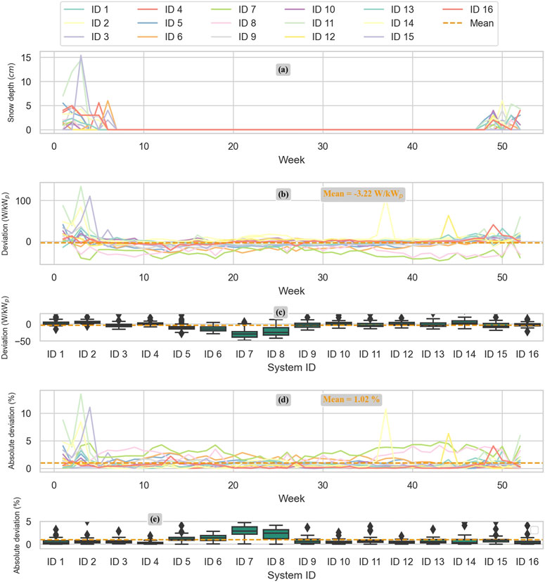
FIGURE 7. Snow deposition information for all 16 real PV systems. Deviation and absolute deviation of 52 days for now-casting for all 16 real PV systems, considering snow deposition. Subplot (A) shows the snow depth in centimeters (cm) for all the locations of the real PV systems. Subplots (B) and (C) show the now-casting deviation (in W/kWp) after the snow information has been considered, and the correction has been performed for each of the 16 real PV systems. Subplots (D) and (E) show the absolute deviation (in %) of now-casting for all 16 PV systems after the correction for snow deposition has been implemented.
Next, we use that linear regression to correct the power forecasted based on the snow information available by location. In Figure 7, it can be observed that the high deviations in winter have been reduced by approximately 75% for some specific cases (see System ID 15). In general, the now-casting mean deviation of all 16 PV systems is −3.22 W/kWp installed, underperforming constantly more evident for some specific PV systems such as PV system ID 6, ID7, and ID8. An absolute deviation of 1.02% can be observed, improving the overall accuracy by 0.79% or 44% relative to the previous calculation by only including snow deposition information for all 16 locations.
The results presented in this work suggested that PV systems with pyranometers as irradiance sensors presented lower deviation than those with reference cells installed as irradiance sensors. As suggested by Rivera and Reise, to further improve the now-casting accuracy and to reduce deviations, corrections can be applied to the values measured by reference cell sensors (Rivera Aguilar and Reise, 2020).
Moreover, additional loss factors that directly impact the power production of a PV system, such as degradation, power clipping, and soiling, could be possibly captured by some of the parameters of the GA optimization, i.e., nominal power and the DC-to-AC ratio. Further investigation is required to confirm these assumptions and improve the model accordingly.
We acknowledge that the GA optimization method presented here has some limitations. In addition to the loss factors mentioned in the aforementioned subsections (degradation, power clipping, and soiling), it is also important to mention that some shading effects, such as inter-row, can directly impact the optimization results. Furthermore, measuring
Although solutions such as GA optimization have been available over an extended period, this work proposes a novel and accurate implementation method for extracting parameters of PV systems or subsystems without prior technical information. The parameters extracted describe the main characteristics of a PV system or subsystem, which later can be translated to a digital twin. The basic parameters of a PV system or subsystem digital twin are defined based on only the on-site measured data in this work.
Based on the experiments presented here, the best condition–training length combination for the GA optimization is defined as all-sky conditions and 182 days long, with only on-site measured data. With the method proposed in this work, a digital twin is created to now-cast with an accuracy of only 0.91% MAPE and 3.27 W/kWp MBE for PV power now-casting.
Furthermore, a validation process is presented, demonstrating the potential of parameterizing a digital twin for each PV plant within a portfolio. A season-independent digital twin is parameterized, and each of the 16 real PV plants distributed in Germany is now-casted with a mean deviation value of −1.14 W/kWp and an MAD of only 1.81%. The model presented here can be further improved to achieve an MAD of only 1.02%, if external locally measured information is considered, i.e., snow precipitation.
The raw data supporting the conclusion of this article will be made available by the authors, without undue reservation.
DG and HM contributed to conceptualization, data processing, simulations, and analyses; CW discussed the results and improved the overall results of this publication. All authors contributed to the article and approved the submitted version.
The authors acknowledge the financial support from the Federal Ministry for Economic Affairs and Energy of Germany (BMWi) in the project ALPRO (project number 0324054A).
The authors declare that the research was conducted in the absence of any commercial or financial relationships that could be construed as a potential conflict of interest.
All claims expressed in this article are solely those of the authors and do not necessarily represent those of their affiliated organizations, or those of the publisher, the editors, and the reviewers. Any product that may be evaluated in this article, or claim that may be made by its manufacturer, is not guaranteed or endorsed by the publisher.
Almeida, M. P., Perpiñán, O., and Narvarte, L. (2015). PV power forecast using a nonparametric PV model. Sol. Energy 115, 354–368. doi:10.1016/j.solener.2015.03.006
Ding, M., Wang, L., and Bi, R. (2011). An ANN-based approach for forecasting the power output of photovoltaic system. Procedia Environ. Sci. 11, 1308–1315. doi:10.1016/j.proenv.2011.12.196
Dirnberger, D., Müller, B., and Reise, C. (2015). PV module energy rating: Opportunities and limitations. Prog. Photovolt. Res. Appl. 23, 1754–1770. doi:10.1002/pip.2618
González Ordiano, J. Á., Waczowicz, S., Reischl, M., Mikut, R., and Hagenmeyer, V. (2017). Photovoltaic power forecasting using simple data-driven models without weather data. Comput. Sci. Res. Dev. 32, 237–246. doi:10.1007/s00450-016-0316-5
Guzman Razo, D. E., Müller, B., Madsen, H., and Wittwer, C. (2020). A genetic algorithm approach as a self-learning and optimization tool for PV power simulation and digital twinning. Energies 13, 6712. doi:10.3390/en13246712
Heydenreich, W., Müller, B., and Reise, C. (2008). “Describing the world with three parameters: A new approach to PV module power modelling,” in 23rd European Photovoltaic Solar Energy Conference and Exhibition, Valencia, Spain, 1-5 September 2008, 2786–2789.
Holland, J. H. (1975). Adaptation in natural and artificial systems: An introductory analysis with applications to biology, control, and artificial intelligence/. Ann Arbor, Michigan: Mich. University of Michigan Press.
Holmgren, W., Calama-Consulting, , Lorenzo, T., Hansen, C., Mikofski, M., Krien, U., et al. (2020). pvlib/pvlib-python: v0.7.1. Zenodo.
Ibrahim, I. A., Mohamed, A., and Khatib, T. (2015). “Modeling of photovoltaic array using random forests technique,” in IEEE Conference on Energy Conversion, Johor Bahru, Malaysia, 19-20 October 2015, 390–393. ed. I. C. o. E. Conversion ([Piscataway, NJ]: IEEE).
IEC (2009). International Standard 61850 - communication networks and systems for power utility automation – Part 7-420: Basic communication structure – distributed energy resources logical nodes. Geneva, Switzerland: Genève: Commission électrotechnique internationale. IEC IEC 61850-7-420 Accessed 2022.
International Energy Agency (2022). Renewables 2022: Analysis and forecast to 2025. Paris, France: IEA.
Jordan, D. C., Kurtz, S. R., VanSant, K., and Newmiller, J. (2016). Compendium of photovoltaic degradation rates. Prog. Photovolt. Res. Appl. 24, 978–989. doi:10.1002/pip.2744
Kaspar, F., Müller-Westermeier, G., Penda, E., Mächel, H., Zimmermann, K., Kaiser-Weiss, A., et al. (2013). Monitoring of climate change in Germany – data, products and services of Germany's National Climate Data Centre. Adv. Sci. Res. 10, 99–106. doi:10.5194/asr-10-99-2013
Landelius, T., Andersson, S., and Abrahamsson, R. (2019). Modelling and forecasting PV production in the absence of behind-the-meter measurements. Prog. Photovolt. Res. Appl. 27, 990–998. doi:10.1002/pip.3117
Mandal, P., Madhira, S. T. S., haque, A. U., Meng, J., and Pineda, R. L. (2012). Forecasting power output of solar photovoltaic system using wavelet transform and artificial intelligence techniques. Procedia Comput. Sci. 12, 332–337. doi:10.1016/j.procs.2012.09.080
Monteiro, C., Fernandez-Jimenez, L. A., Ramirez-Rosado, I. J., Muñoz-Jimenez, A., and Lara-Santillan, P. M. (2013). Short-term forecasting models for photovoltaic plants: Analytical versus soft-computing techniques. Math. Problems Eng. 2013, 1–9. doi:10.1155/2013/767284
Mori, N., and Kita, H. (2000). “Genetic algorithms for adaptation to dynamic environments - a survey,” in IECON 2000: 26th annual conference of the IEEE Industrial Electronics Society (IEEE), Nagoya, Japan, 22-28 October 2000, 2947–2952.
Müller, B., Hardt, L., Armbruster, A., Kiefer, K., and Reise, C. (2016). Yield predictions for photovoltaic power plants: Empirical validation, recent advances and remaining uncertainties. Prog. Photovolt. Res. Appl. 24, 570–583. doi:10.1002/pip.2616
Müller, B., Reise, C., Heydenreich, W., and Kiefer, K. (2007). Are yield certificates reliable? A comparison to monitored real world results. Washington, United States: Health IT. Unpublished.
Ogliari, E., Dolara, A., Manzolini, G., and Leva, S. (2017). Physical and hybrid methods comparison for the day ahead PV output power forecast. Renew. Energy 113, 11–21. doi:10.1016/j.renene.2017.05.063
Reno, M. J., and Hansen, C. W. (2016). Identification of periods of clear sky irradiance in time series of GHI measurements. Renew. Energy 90, 520–531. doi:10.1016/j.renene.2015.12.031
Rivera Aguilar, M. J., and Reise, C. (2020). “Silicon sensors vs. Pyranometers – review of deviations and conversion of measured values,” in 37th European Photovoltaic Solar Energy Conference and Exhibition, Marseille, France, September 2020, 1449–1454.
Schmidt, H., and Sauer, D. (1994). Wechselrichter-Wirkungsgrade - praxisgerechte Modellierung und Abschätzung. Sonnenenerg 1996.
SolarPower Europe, (2022). Global market outlook for solar power 2022-2026. Bruxelles, Belgium: SolarPower Europe.
Stein, J. S., Hansen, C. W., and Reno, M. J. (2012). Global horizontal irradiance clear sky models: Implementation and analysis. OSTI.
Urraca, R., Huld, T., Lindfors, A. V., Riihelä, A., Martinez-de-Pison, F. J., and Sanz-Garcia, A. (2018a). Quantifying the amplified bias of PV system simulations due to uncertainties in solar radiation estimates. Sol. Energy 176, 663–677. doi:10.1016/j.solener.2018.10.065
Keywords: machine learning, genetic algorithms, auto-calibrated algorithms, photovoltaic systems, parameter estimation, digital twin, PV power forecasting, PV system modeling
Citation: Guzman Razo DE, Madsen H and Wittwer C (2023) Genetic algorithm optimization for parametrization, digital twinning, and now-casting of unknown small- and medium-scale PV systems based only on on-site measured data. Front. Energy Res. 11:1060215. doi: 10.3389/fenrg.2023.1060215
Received: 03 October 2022; Accepted: 15 May 2023;
Published: 01 June 2023.
Edited by:
Mohammadreza Aghaei, Norwegian University of Science and Technology, NorwayReviewed by:
Atse Louwen, Eurac Research, ItalyCopyright © 2023 Guzman Razo, Madsen and Wittwer. This is an open-access article distributed under the terms of the Creative Commons Attribution License (CC BY). The use, distribution or reproduction in other forums is permitted, provided the original author(s) and the copyright owner(s) are credited and that the original publication in this journal is cited, in accordance with accepted academic practice. No use, distribution or reproduction is permitted which does not comply with these terms.
*Correspondence: Dorian Esteban Guzman Razo, ZG9yaWFuZWd1em1hbkBnbWFpbC5jb20=
Disclaimer: All claims expressed in this article are solely those of the authors and do not necessarily represent those of their affiliated organizations, or those of the publisher, the editors and the reviewers. Any product that may be evaluated in this article or claim that may be made by its manufacturer is not guaranteed or endorsed by the publisher.
Research integrity at Frontiers
Learn more about the work of our research integrity team to safeguard the quality of each article we publish.