 Jinping Duan1
 Xiaoxue Huang2*
- 1State Key Laboratory of Nuclear Power Safety Monitoring Technology and Equipment, China Nuclear Power Engineering Co, Ltd, Shenzhen, Guangdong, China
- 2Department of Mechanical Engineering, The University of Sheffield, Sheffield, United Kingdom
Thermal striping in a T-junction with sodium streams mixing at different temperatures is studied using unsteady Reynolds-averaged simulation (RANS). Different parameters including the momentum ratio of the streams (0.2–4.3), the temperature difference between the streams (15–35 K), and the bulk Reynolds number (5,000–9,000) are investigated. Simulation results demonstrate that the flow pattern is mainly determined by the momentum ratio, while the temperature difference and the bulk Reynolds number have little influence within the range considered. The location of the separation point of the recirculation zone increases with the momentum ratio while the location of the thermal front decreases with it. In addition, the sensitivity of the temperature fluctuations to a range of low-Reynolds-number turbulence models are studied, which demonstrate that the time-varying temperature fluctuations predicted by these turbulence models are significantly smaller than the experimental measurements. High-fidelity simulations which fully resolve the temperature fluctuations will be carried out as the future work to complement the statistics of the temperature fluctuation.
1 Introduction
Thermal striping is often observed in the piping of liquid metal-cooled fast reactors (LMFRs) where two or more fluid streams at different temperatures meet. This is characterized by temperature fluctuations which can potentially cause cyclical thermal stresses and therefore fatigue cracking of the structures. Prediction of the thermal fatigue in the mixing region is important as it is important in terms of life cycle management of the piping systems.
Studies of thermal mixing in T-junctions have been reported by many authors (Lee et al., 2009; Walker et al., 2009; Ndombo and Howard, 2011; Gauder et al., 2016; Zhou et al., 2018). The complex features such as secondary flow, separation, recirculation, and reattachment have been investigated. Walker et al. (2009) studied the scalar mixing of water and identified four characteristic regions in the vicinity of the junction interface. It comprises a mixing region with high fluctuations, a recirculation region containing two contra-rotating vortices, and two regions with small fluctuations. Ndombo and Howard (2011) examined the effect of the inlet turbulence on the unsteadiness of the flow. The turbulence at the inlet does not seem to have significant effect on the bulk flow, whereas it influences the near-wall flow, i.e., the wall temperature fluctuation and the temperature-velocity correlation are moved downstream with reduced magnitude with the inclusion of turbulence at the inlet. Similar results were presented by Gauder et al. (2016) through comparing the simulation results with and without turbulence at the inlets. Zhou et al. (2018) carried out experiments to investigate the thermal mixing with varied temperature differences. The temperature difference ranges from 140 K to 220 K and it has been found the temperature difference has a significant influence on the thermal stratification in the mixing flow as well as the reverse flow, and thus a significant influence on the thermal fatigue in the T-junction. Numerical analysis carried out by Lee et al. (2009) also identified the temperature difference (up to 150 K) between the two streams as the dominant factor among various parameters that affects the thermal fatigue. It is established that high-fidelity simulations such as large eddy simulation (LES) can capture the unsteadiness, which is responsible for the mechanical stresses that cause the thermal fatigue, whereas RANS (Reynolds Averaged Navier Stokes) models or URANS (Unsteady RANS) models to calculate the mean temperature and the temperature variance has been found unable to directly identify the local fluctuations associated with the thermal mixing.
In liquid metal-cooled fast reactors, there are several areas susceptible to thermal striping where hot and cold fluids merge, including the core outlet region, the upper plenum, and the flow guide tube, etc. Due to the high-temperature, opaque, and corrosive features of liquid metal experiments, the record of experimental data of liquid metal is scarce and most experimental studies use water as the working fluid. The large diffusivity for heat and the small diffusivity for momentum makes the liquid metal convection different from ordinary fluid convection, such as water. It has been shown that the results of water are not transferable to liquid metal especially under mixed convection as the velocity field depends strongly on the temperature field and the heat transfer behavior is significantly different from that of fluids at higher Prandtl number due to the dominance of molecular diffusion in heat transport (Huang and He, 2022a; Huang and He, 2022b). Dimensional analysis and experimental study have shown that the spectral distribution of temperature fluctuations of low Prandtl number fluids displays different characteristics compared with that of water (Bremhorst and Krebs, 1992). On the other hand, turbulence modelling of liquid metal convection is a topic requiring thorough investigation as the low Prandtl number induces different scales of the velocity field and the temperature field (Kawamura et al., 2000; Otic and Grötzbach, 2007). The properties of liquid metal pose difficulties on the turbulence modelling as the widely employed assumptions such as Reynolds analogy may not be applicable to liquid metal convection (Arien, 2002; Grötzbach, 2007; Shams, 2018). Otic and Grötzbach (2007) demonstrated incomplete modelling of turbulence heat flux with eddy diffusivity model. Roelofs et al. (2019) summarized dissimilarity in velocity and thermal fields for liquid metal as the wall layer thickness and the fluctuation fields do not behave similarly. Kawamura et al. (2000) performed direction numerical simulation of forced convection and demonstrated that the timescale ratio shows similar behavior in the near-wall region while it depends significantly on the boundary conditions in the bulk region. Otic and Grotzbach showed that using a thermal timescale or combining thermal and mechanical timescales improves the modelling of the turbulent heat transport in Rayleigh-Benard convection (Otić et al., 2005). Different approaches to model the turbulent heat transfer have been developed for liquid metal flows (Carteciano and Groetzbach, 2003; Manservisi and Menghini, 2014), however, further development and validation is still needed for complex configurations and for all flow regimes.
This paper investigates the thermal mixing in the T-junction. The computational model replicates the geometry and the experimental conditions of a rig detailed in Weathered (2017). A range of low-Reynolds-number turbulence models are employed, and the experimental data are used to compare with the simulation results. This is a preliminary numerical investigation of the thermal stripping phenomenon of sodium with a focus on the parametrical study and the performance estimation of various turbulence models.
2 Methodology
2.1 Experimental setup
A schematic of the T-junction is given in Figure 1. The test section has two streams of sodium impinging onto each other at different temperatures and flow rates. The temperature difference and the flow rates were varied to parametrically study the thermal striping phenomenon. Optical fibre sensors were employed for the temperature measurements in the experiments. The vertical main pipe with diameter of 22.1 mm delivered hot sodium, and the horizontal branch pipe with diameter of 7 mm delivered cold sodium. The entry length of the main pipe is 308 mm. The vertical length from the branch pipe to the exit of the main pipe is 221 mm, which is 10 times of the diameter. The entry and the exit lengths ensure sufficiently developed upstream and downstream flows.
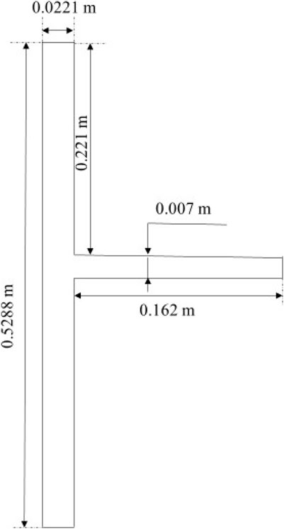
FIGURE 1. Schematic of the simulation domain of T-junction.
2.2 Turbulence models
The unsteady RANS equations for the flow are expressed as follows:
Where
The Launder-Sharma k-ε model differs from the standard k-ε model as damping functions to account for the viscous and wall effects are included. The k-ω SST model uses a standard k-ω closure in the near-wall region and a k-ε model in the free-shear region. The v2-f model can be considered as a k-ε model with wall-normal stress anisotropy by solving an additional transport equation for the wall-normal stress.
Reynolds-stress models (RSMs) solve a transport equation for each stress component. The elliptic blending Reynolds-stress model (EBRSM) which solves an elliptic equation for the pressure-strain term in the near-wall and the outer region is employed. The low-Re variant of RSM accounts for the difference in the turbulence near the wall and that at some distances away from the wall.
The simulations are carried out using Code_Saturne, version 6.0.8, an open-source finite volume solver developed by Electrictite de France (EDF) (EDF R&D, 2019). Second order centered scheme is employed for spatial and temporal discretization. The solver of the linear system is Jacobi for velocity and temperature, algebraic multigrid for pressure.
2.3 Mesh setup
The mesh is generated with the first cell wall spacing y+≤1 to resolve the viscous sublayer and 5–10 cells placed below y+ = 20. The total number of elements of the mesh is 601,008 (shown in Figure 2). In the streamwise and the transverse directions, the sizes ∆x and ∆z are kept under 40 and 20, respectively. A mesh independence study has been carried out prior to the simulation. Temperature at selected downstream locations were monitored and it demonstrated that the solution is invariant when the mesh is further refined.
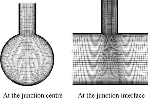
FIGURE 2. Mesh for the T-junction (full inlets and outlets have been cropped).
2.4 Thermophysical properties
The thermophysical properties of sodium are taken from Sobolev (2011). Table 1 gives the details of the properties.
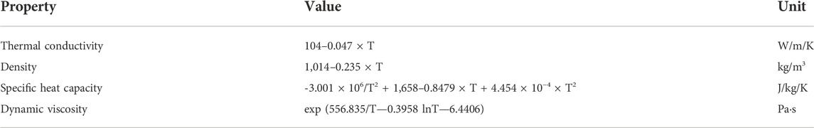
TABLE 1. Properties of liquid sodium.
2.5 Boundary conditions
Volumetric flow rate and constant temperature are prescribed at both inlets, a free outlet, i.e., zero-flux condition for the velocity and the temperature is prescribed at the outlet. Table 2 gives details of eight cases for the simulation.
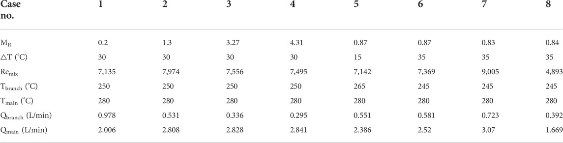
TABLE 2. Parameters of the simulation cases.
To fully characterize thermal striping at the T-junction, the relevant parameters including the Momentum Ratio (MR), the temperature difference (∆T) between the main pipe and the branch pipe, and the bulk Reynolds number (Remix) are varied.
The momentum is defined as the volumetric flow rate multiplied by the momentum per unit volume. MR is thus given as follows
where
The inlet flow rates range from 1.67 L/min to 3.07 L/min at the main pipe and 0.3 L/min to 0.98 L/min at the branch pipe, thus the range of Remix is 4,900 to 7,000. The range of the temperature difference between the main pipe flow and the branch pipe flow is 15°C to 35°C.
Among the eight cases, cases 1–4 vary the MR, cases 5–6 vary ∆T, cases 7–8 vary Remix.
3 Results
This section details the simulation results of the T-junction. The results in Section 3.1, 3.2 employ k-ω SST model, and a comparison of different turbulence models (EBRSM, k-ω SST, Launder-Sharma k-ε and v2-f) is presented for Case 1 in Section 3.3. The time step size is 0.01s and the Courant number is kept lower than 1. Time-averaged data are collected for 50 flow through times after the domain reaches a statistically converged state, i.e., when the mean temperature value at the outlet keeps unchanged.
Time-averaged temperature and jet trajectory of cases 1–4 are compared against experimental results for investigation of the general flow patterns of the jet with various momentum ratios. Line plots of temperature, velocity and shear stress along the centerline and the near side wall of the main pipe are presented to investigate the locations of the thermal front of the jet and the size of the recirculation zone. The turbulent kinetic energy (indications of the level of turbulent temperature fluctuations, i.e., small-scale fluctuations), and the time variations of temperature (represent large-scale fluctuations in temperature) are given together with the experimentally measured peak-to-peak temperature variations for understanding of the thermal striping locations and levels.
Section 3.1 gives the results of cases 1–4, Section 3.2 gives the results of cases 5–8. In addition, a comparison between various low-Re turbulence models for case 1 is given in Section 3.3.
3.1 Results with various momentum ratios
The normalized mean temperature is defined as follows
Where
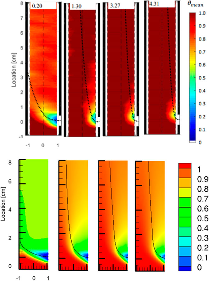
FIGURE 3. Normalized mean temperature for various momentum ratios. Top row: results from experiments, predicted jet trajectories displayed with dotted black lines. Bottom row: results from simulations (cases 1–4 from left to right), jet trajectories displayed with solid black line.
The jet trajectory is defined as the location of the maximum velocity of the downstream flow, thus it defines the flow path of it. In the simulation results, the trajectory is denoted by the stream trace from the centerline of the branch pipe. In the experimental results, the predicted trajectory shown was calculated using a correlation for the trajectory of a jet from a junction positioned flush with a flat plate (Kamotani and Greber, 1974). The correlation is given as
where
The top row in Figure 3 shows the experimental results (Weathered, 2017). MR of different cases are labelled on the top of each contour plot. The bottom row shows the simulation results of cases 1–4. As shown both from the experiments and the simulations, the flow pattern changes from impinging jet to wall jet with MR increasing from 0.2 to 4.31, which is consistent with the flow categories in literature (Hosseini et al., 2008). A reasonable agreement is observed between the simulations and the experiments in terms of the mean temperature.
The jet trajectories in the simulations differ from the trajectories predicted by Eq. 5 as they generally shift towards the far side wall in the simulations. This can be attributed to the different configurations between the simulation and the experiment in Kamotani and Greber (1974). In the simulation, the branch jet flow mixes with the pipe flow in the main pipe, whereas in the experiment in Kamotani and Greber (1974), the branch flow mixed with the cross flow over a flat plate. Besides, buoyancy effects may also contribute to this difference as Eq. 5 does not include the influence of buoyancy while the simulation has non-negligible buoyancy effect due to thermal mixing. An estimation of the trajectory location at 8 cm downstream from the branch pipe, i.e., the exit location of the trajectory in the figure, is made. It is found to be −0.122, 0.255, and 0.345 cm from the centerline of the pipe (the negative sign indicates further away from the jet side) in the experiments, compared to −0.539, −0.225, and −0.166 cm in the simulations (cases 2–4).
Figure 4 shows the temperature and streamwise velocity along the centerline of the main pipe. Following an increase in the velocity close to the junction interface due to the mixing of the streams, the velocity decreases as a result of the fast decay of the jet and increases again in cases 1 and 2 as the impinged jet mixes with the main pipe flow again. Correspondingly, the temperature decreases at the beginning due to the cold branch flow then increases due to the thermal mixing of the two streams.
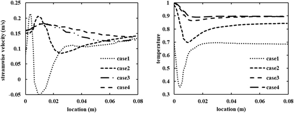
FIGURE 4. Streamwise velocity (left) and normalized temperature (right) along the centerline of the main pipe for cases 1–4.
Figure 5 shows the wall shear stress and the normalized temperature along the near side wall for cases 1–4. A recirculation zone is formed where the wall shear stresses are negative at the side wall. The location of the separation point between the recirculation zone and the upward main flow where the wall shear stress is zero is given in Table 3 for cases 1–4. The temperature increases monotonically along the near side wall as the two streams mix. The thermal front of the jet is defined as the location where the normalized mean temperature is 0.8. In case 1, the temperature has not reached 0.8 before the impingement. In cases 2–4, the thermal front predicted by the simulations and that estimated from the contour plots of experiments are given in Table 3. It is worth pointing out that the contour plots for the experiments in Figure 3 were interpolated from the measurements and uncertainties in the thermal front location in experiments may arise from the interpolation.
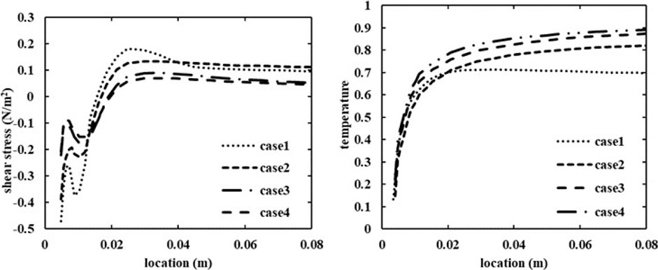
FIGURE 5. Wall shear stress (left) and normalized temperature (right) along the near side wall of the main pipe for cases 1–4.
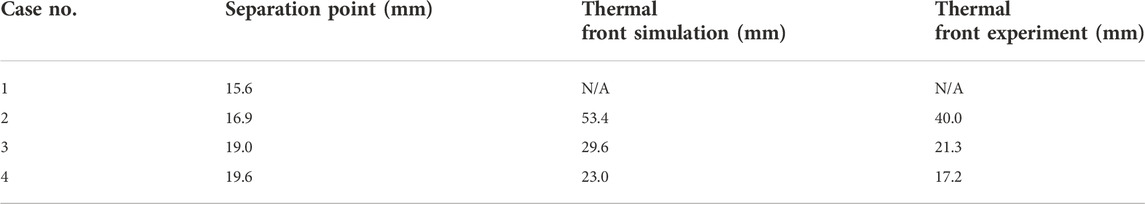
TABLE 3. Locations of the separation point and the thermal front for Cases 1– 4.
The time-dependent temperature data was collected by the optical fiber. The peak-to-peak normalized temperature range was calculated as
where
The temperature fluctuations captured by experiments cannot be resolved directly in the turbulence modelling as the temperature fluctuation variance (
For an indicative comparison with the experiments, TKE (normalized by velocity squared) is shown in Figure 6 to demonstrate the level of turbulence over the domain. The distribution of TKE largely follows the streamline as a result of shearing between the jet and the main pipe flow. The TKE level in case 1 is the highest as the shear flow is strong due to the low MR of the main flow over the branch flow. In each case, the highest TKE is seen slightly downstream from the trajectories as the recirculation zone is formed in those regions.
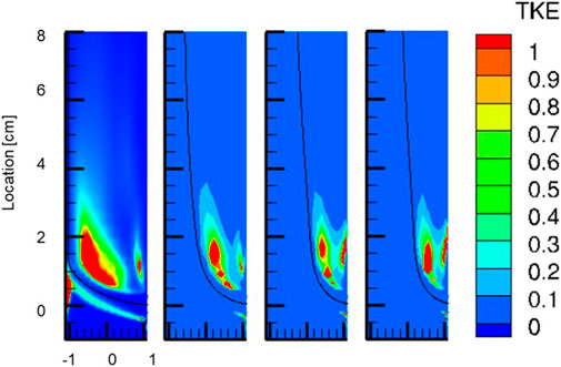
FIGURE 6. Turbulent kinetic energy (0.5<
The temperature variations with time predicted by the URANS models are not significant (lower than 1K) in the current simulations, showing that the k-ω SST model is not able to predict the large-scale temperature fluctuations. A comparison of different URANS models in terms of this time-varying temperature fluctuation will be given in this Section 3.3.
3.2 Results with various temperature differences and bulk Reynolds numbers
Figure 7 gives the normalized mean temperature distribution of cases 5–8. A turning jet is observed in these cases as the MR is fixed at 0.85. Figure 8 shows the wall shear stress and the temperature along the near side wall. The wall shear stress increases with the Remix comparing cases∼8), however, it does not vary significantly with the ∆T (cases 5–6). The locations of the separation points are given in Table 4. The normalized temperature profiles collapse together for cases 5–8 as shown in Figure 8, therefore, the locations of the thermal fronts for those cases are almost the same and not included in Table 4 for comparison.
3.3 Comparison of different turbulence Models
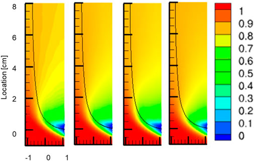
FIGURE 7. Normalized mean temperature contour plots for different temperature difference and mixed Reynolds number. Results from simulations (cases 5–8 from left to right), jet trajectories displayed with solid black line.
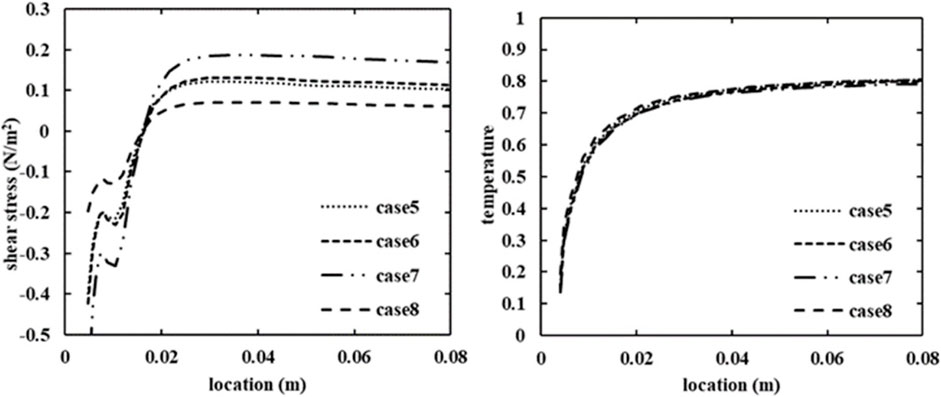
FIGURE 8. Wall shear stress and normalized temperature along the near side wall of the main pipe for cases 5–8.

TABLE 4. Locations of the separation point and the thermal front for Cases 5–8.
A comparison of different turbulence models has been conducted using the boundary conditions of case 1. This case has been selected for comparison as temperature fluctuations observed are strong at both the far side wall and the near side wall in the experiments.
The results of case 1 with various turbulence models are shown in Figures 9–11. The mean temperature distributions are largely the same for the tested turbulence models. Therefore, the contour plots of temperature are omitted and the plots of total shear stress and temperature along the near side wall are shown in Figure 9 instead. Besides, the locations of the separation point, and the thermal front produced by different turbulence models are almost the same. The wall shear stress in the recirculation center is the highest with v2-f model and lowest with the LS k-ε turbulence model.
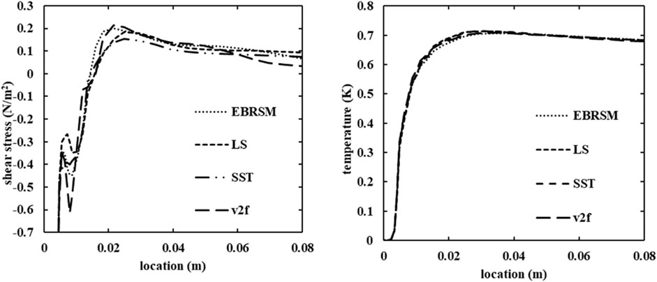
FIGURE 9. Wall shear stress and temperature along the near side wall of the main pipe in the simulations using different turbulence models.
Figure 10 shows the TKE distribution for the tested turbulence models. The LS k-ε turbulence model predicted the strongest turbulence level, while EBRSM and v2-f produce a low level of turbulence.
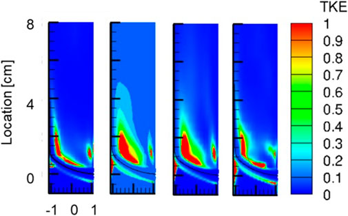
FIGURE 10. TKE in the simulations using different turbulence models (from left to right: EBRSM, LS k-ε and k-ω SST, v2-f).
Figure 11 shows the time variation of the temperature at different locations. Three locations are monitored: 1D downstream at the near side wall, 0D downstream at the centerline and 0D downstream at the far side wall (D is the diameter of the main pipe). Among the tested turbulence models, k-ω SST is not able to reproduce the large-scale temperature fluctuations, while LS k- ε produces the strongest temperature fluctuations. The middle location, i.e., the location at the centerline, has shown low frequency with high magnitude of temperature variations, whereas the far location, i.e., the location at the far side wall, is comparatively silent. Correspondingly, the TKE level at the far location is high while it is relatively low at the middle location as shown in Figure 10. In the results from EBRSM and v2-f, the difference between the three locations is not as significant as that in the LS k-ε result.
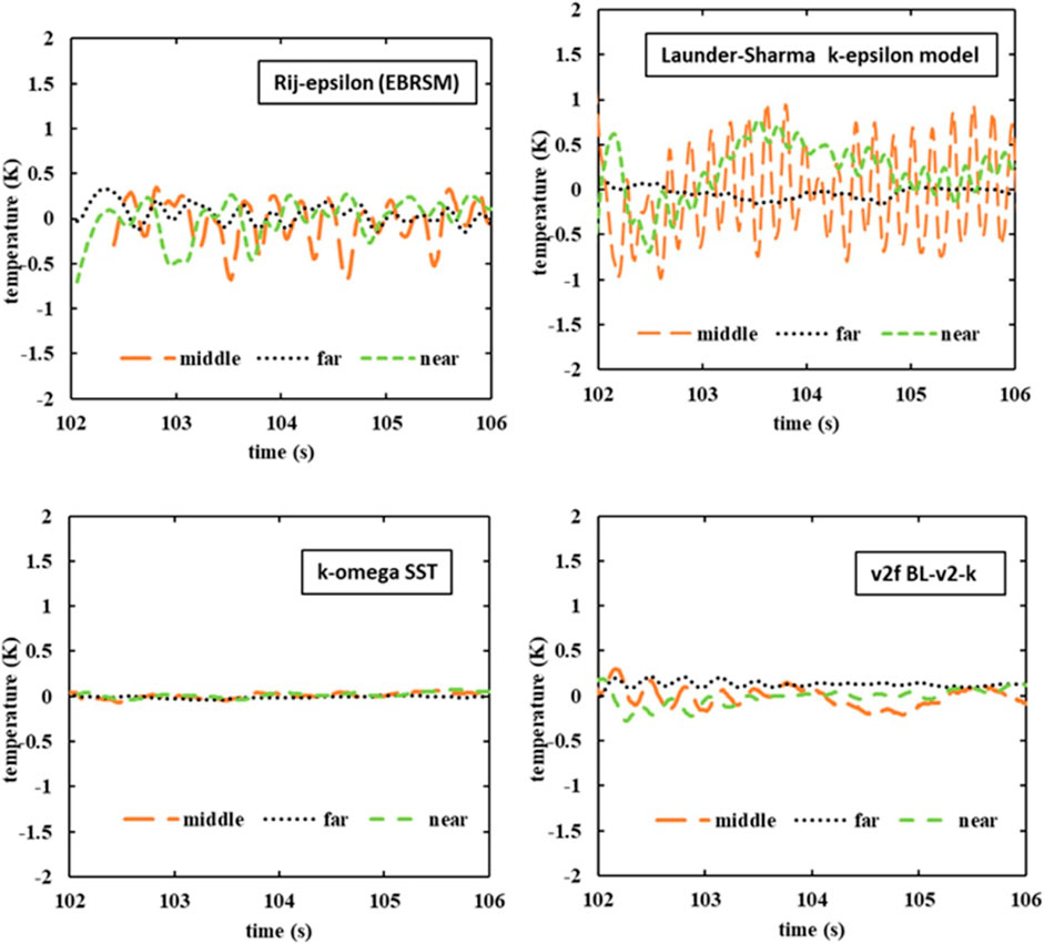
FIGURE 11. Temperature variations with time with different turbulence models.
According to the experimental results of the peak-to-peak temperature range in Weathered (2017), the fluctuation level is around 50% of the temperature difference (i.e., about 15 K), however, the simulation predicted temperature variation is just around 1 K in the case with strongest temperature fluctuations, i.e., the case using LS k-ε model. LES or unsteady RANS with transport equations for the temperature invariance and turbulent heat flux are needed for such predictions and this is the next step of the current study.
4 Conclusion
Unsteady RANS studies have been carried out for the thermal striping phenomena of a non-isothermal T-junction at various momentum ratios, temperature differences and bulk Reynolds numbers. The sensitivity to different turbulence models is also investigated. The main conclusions are as follows:
Within the range of the parameters considered, the flow pattern, including the distribution of the mean temperature, distribution of the recirculation zone and the location of the thermal front, is mainly determined by the momentum ratio while the temperature difference and the bulk Reynolds number have little influence. The location of the separation point of the recirculation zone increases with the momentum ratio while the location of the thermal front decreases with it.
According to the experiments, the temperature fluctuation level is around 50% of the temperature difference and it increases with the momentum ratio. Such fluctuations cannot be resolved directly in URANS simulations. Instead, the small-scale (turbulent) fluctuations can be indirectly inferred from TKE, whereas the large-scale fluctuations can be directly resolved and represented by the unsteady temperature variations. The simulation results show that the TKE level decreases with the momentum ratio. The TKE level is high in the cases with Launder-Sharma k-ε and k-ω SST compared to the rest of the turbulence models. On the other side, the time-varying temperature fluctuations predicted in the case with Launder-Sharma k-ε is the highest (but still around 1K) and it is nearly 0 in the case with k-ω SST.
LES simulations and URANS simulations with transport equations for the temperature invariance and turbulent heat flux are undertaken to directly resolve the temperature fluctuations associated with thermal striping as the next step of this study.
Data availability statement
The original contributions presented in the study are included in the article/Supplementary Material, further inquiries can be directed to the corresponding author.
Author contributions
JD: Conceptualization, Methodology, and Investigation. XH: Data curation and Writing.
Funding
This work has been performed using resources provided by the Cambridge Tier-2 system operated by the University of Cambridge Research Computing Service (www.hpc.cam.ac.uk) funded by EPSRC Tier-2 capital grant EP/P020259/1.
Conflict of interest
Author JD was employed by China Nuclear Power Engineering Co, Ltd.
The remaining authors declare that the research was conducted in the absence of any commercial or financial relationships that could be construed as a potential conflict of interest.
Publisher’s note
All claims expressed in this article are solely those of the authors and do not necessarily represent those of their affiliated organizations, or those of the publisher, the editors and the reviewers. Any product that may be evaluated in this article, or claim that may be made by its manufacturer, is not guaranteed or endorsed by the publisher.
References
Arien, B. (2002), Assessment of computational fluid dynamics codes for heavy liquid metals, Mol, Belgian: ASCHLIM EC-Con. FIKW-CT-2001-80121-Final Report.
Bremhorst, K., and Krebs, L. (1992). Experimentally determined turbulent Prandtl numbers in liquid sodium at low Reynolds numbers. Int. J. Heat. Mass Transf. 35 (2), 351–359. doi:10.1016/0017-9310(92)90273-u
Carteciano, L. N., and Groetzbach, G. (2003). Validation of turbulence models in the computer Code FLUTAN for a free hot sodium jet in different buoyancy flow regimes. Germany: ETDEWEB.
Gauder, P., Selvam, P. K., Kulenovic, R., and Laurien, E. (2016). Large eddy simulation studies on the influence of turbulent inlet conditions on the flow behavior in a mixing tee. Nucl. Eng. Des. 298, 51–63. doi:10.1016/j.nucengdes.2015.12.001
Grötzbach, G. (2007). Anisotropy and buoyancy in nuclear turbulent heat transfer – critical assessment and needs for modelling. FZKA: Forschungszentrum Karlsruhe.
Hosseini, S. M., Yuki, K., and Hashizume, H. (2008). Classification of turbulent jets in a T-junction area with a 90-deg bend upstream. Int. J. Heat Mass Transf. 51 (9-10), 2444–2454. doi:10.1016/j.ijheatmasstransfer.2007.08.024
Huang, X., and He, S. (2022). Study of a lead-bismuth eutectic jet issued into a heated cavity using large eddy simulation. Int. J. Heat Mass Transf. 198, 123407. doi:10.1016/j.ijheatmasstransfer.2022.123407
Huang, X., and He, S. (2022). Study of a negatively buoyant jet of liquid metal in a density-stratified ambient. Int. Commun. Heat Mass Transf. 138, 106351. doi:10.1016/j.icheatmasstransfer.2022.106351
Kamotani, Y., and Greber, I. Experiments on confined turbulent jets in cross flow (1974). Technical report, Cleveland: Case Western Reserve University,
Kawamura, H., Abe, H., and Shingai, K. (2000). DNS of turbulence and heat transport in a channel flow with different Reynolds and Prandtl numbers and boundary conditions, 3rd International Symposium on Turbulence. Nagoya, Japan: Heat Mass Transf.
Lee, J. I., Hu, L., Saha, P., and Kazimi, M. S. (2009). Numerical analysis of thermal striping induced high cycle thermal fatigue in a mixing tee. Nucl. Eng. Des. 239 (5), 833–839. doi:10.1016/j.nucengdes.2008.06.014
Manservisi, S., and Menghini, F. (2014). Triangular rod bundle simulations of a CFD κ-ϵ-κθ-ϵθ heat transfer turbulence model for heavy liquid metals. Nucl. Eng. Des. 273, 251–270. doi:10.1016/j.nucengdes.2014.03.022
Ndombo, J., and Howard, Richard J. A. (2011). Large Eddy Simulation and the effect of the turbulent inlet conditions in the mixing Tee. Nucl. Eng. Des. 241 (6), 2172–2183. doi:10.1016/j.nucengdes.2011.03.020
Otic, I., and Grötzbach, G. (2007). Turbulent heat flux and temperature variance dissipation rate in natural convection in lead-bismuth. Nucl. Sci. Eng. 155, 489–496. doi:10.13182/nse07-a2679
Otić, I., Grötzbach, G., and Wörner, M. (2005). Analysis and modelling of the temperature variance equation in turbulent natural convection for low-Prandtl-number fluids. J. Fluid Mech. 525, 237–261. doi:10.1017/s0022112004002733
Roelofs, F., Gerschenfeld, A., Tarantino, M., Van Tichelen, K., and Pointer, W. D. (2019). Thermal-hydraulic challenges in liquid-metal-cooled reactors. Sawston, United Kingdom: Woodhead Publishing.
Shams, A. (2018). Towards the accurate numerical prediction of thermal hydraulic phenomena in corium pools. Ann. Nucl. Energy 117, 234–246. doi:10.1016/j.anucene.2018.03.031
Sobolev, V. (2011). Database of thermophysical properties of liquid metal coolants for GEN-IV. 2nd ed. Belgium: SCK·CEN.
Walker, C., Simiano, M., Zboray, R., and Prasser, H. M. (2009). Investigations on mixing phenomena in single-phase flow in a T-junction geometry. Nucl. Eng. Des. 239 (1), 116–126. doi:10.1016/j.nucengdes.2008.09.003
Weathered, M. (2017). “Characterization of sodium thermal hydraulics with optical fiber temperature sensors,”. Thesis (Ph.D.) (Madison: University of Wisconsin).
Keywords: liquid metal-cooled fast reactor, T-junction, URANS, thermal stripping, thermal mixing
Citation: Duan J and Huang X (2023) An unsteady RANS study of thermal striping in a T-junction with sodium streams mixing at different temperatures. Front. Energy Res. 10:991763. doi: 10.3389/fenrg.2022.991763
Received: 11 July 2022; Accepted: 28 September 2022;
Published: 10 January 2023.
Edited by:
Songbai Cheng, Sun Yat-Sen University, ChinaReviewed by:
Shuo Li, The University of Tokyo, JapanTing Zhang, Kyushu University, Japan
Shangzhen Xie, Wuhan Institute of Technology, China
Copyright © 2023 Duan and Huang. This is an open-access article distributed under the terms of the Creative Commons Attribution License (CC BY). The use, distribution or reproduction in other forums is permitted, provided the original author(s) and the copyright owner(s) are credited and that the original publication in this journal is cited, in accordance with accepted academic practice. No use, distribution or reproduction is permitted which does not comply with these terms.
*Correspondence: Xiaoxue Huang, eGlhb3h1ZS5oaUBnbWFpbC5jb20=, eGlhb3h1ZS5odWFuZ0BzaGVmZmllbGQuYWMudWs=