Forecasting crude oil prices volatility by reconstructing EEMD components using ARIMA and FFNN models

The energy sector which includes gas and oil is concerned to explore and develop refined oil and it’s a multitrillion business. As crude oil is a very important source of energy, and it has a very valuable impact on a country’s economic growth, national security, and social stability. Therefore, accurately predicting the crude oil price volatility is a very important topic of research and still, it is a challenge for researchers to accurately forecast crude oil prices. Therefore, this study is conducted to address the said problem significantly. This research presents a novel hybrid method for reconstructing EEMD IMFs that involves two steps. Visual analysis of Average Mutual Information (AMI) graphs were used to rebuild IMFs. EEMD IMFs were split into two components called stochastic and deterministic. In the proposed method, reconstruction of IMFs of EEMD was done at two stages to see if the stochastic components have more variation. Later, ARIMA and FFNN models were used to test the suggested method’s performance. For this purpose, Brent crude oil prices data was used, and the hybrid model EEMD-S2D1D2-ARIMA/FFNN outperformed the other existing hybrid model with minimum MAE = 0.2323, RMSE = 0.3058 and MAPE = 0.5273. A simulation study was also conducted to check the robustness of the proposed method for N = 50, 500, 1,000, 2000, 5,000, and 7,500. The simulation results also confirm that the unpredictability present in the reconstructed IMFs of the hybrid models EEMD-ARIMA/FFNN and EEMD-SD-ARIMA/FFNN has been reduced by the proposed hybrid models.

1 Introduction

Accurately predicting the crude oil price volatility is a very important topic of research because every country’s economy highly depends on crude oil prices. Many factors put a significant impact on crude oil prices such that supply and demand (Kilian, 2009), US dollar exchange rate (Lizardo and Mollick, 2010), venture trading(Kilian and Murphy, 2014), geographically conflicts, and natural disasters (Sahir and Qureshi, 2007) these factors introduce a high level of noise to crude oil prices which consists of non-linearity and uncertain characteristics, which become difficult to forecast. Therefore, crude oil price forecasting remains a huge challenge for all researchers. There are two types of econometric models 1) structural and 2) time series.

The structural model includes the Error Correction Model (ECM), Vector Error Correction Model (VECM), and Vector Auto-Regressive (VAR) model. These models use linear regression and are based on data such as demand and supply. These models also include other explanatory variables in addition to prior data on oil prices. The other technique is time series models, which use just the previous history of oil prices to predict future oil prices. However, these models need data to be stationary and linear because these models cannot accurately deal with the inner complexity of crude oil prices in addition to econometric methodologies.

Xiang and Zhuang (2013) applied the ARIMA model of order (1,1,1) to Brent oil prices from November 2012 to April 2013 and found that the ARIMA model had a good prediction effect and could be used for short-term crude oil price forecasting. Xie et al. (2006) used WTI monthly crude oil prices (COPs) from January 1970 to December 2003 and they applied the support vector regression (SVR) model, the empirical finding showed that the SVR model is more appropriate than ARIMA and Back Propagation Neural Network (BPNN) models in predicting monthly WTI prices. Movagharnejad et al. (2011) employed an ANN model. Kamdem et al. (2020) employed a deep learning model (DLM) for commodities price predictions. Their findings showed that the coronavirus has an impact on commodity price which results in variability. They also utilized an ARIMA-wavelet hybrid model to predict the spread of the coronavirus. The findings revealed a strong link between the spread of the Coronavirus and commodities prices. Yu et al. (2008) used EMD to decompose WTI and Brent daily COPs for the period 20 May 1987 to 30 September 2008, and the findings showed that the decomposition and ensemble techniques worked well and enhanced the models’ performance. Lin and Sun (2020) used CEEMDAN and MLGRU Neural Network and found that the new model improved predicting accuracy for predicting COPs. Wu et al. (2019) also proposed a unique EEMD and LSTM-based technique. The proposed hybrid model was applied to WTI COPs, and the results confirmed the new technique’s superiority. AAMIR (2018) introduced a new method for the reconstruction of IMFs. For reconstruction, the proposed method exploited autocorrelation for the reconstruction of EEMD IMFs. The daily and weekly prices of Brent and WTI were used to assess ARIMA and ANN models’ forecasting performance using reconstructed data. In comparison to single models utilizing ARIMA and FFNN, the proposed approach of reconstruction of IMFs with autocorrelation was found to be the best alternative. Moshiri and Foroutan (2006) employed the ANN model to estimate daily crude oil futures prices traded at the New York Mercantile Exchange (NYMEX). Mostafa and El-Masry (2016) used gene expression programming (GEP) and ANN to forecast the upward and downward movement of oil prices, The least squares support vector machine (LSSVM) approach to oil futures price forecasting was proposed by (Yusof and Mustaffa, 2016). Zhao et al. (2017) proposed a deep learning approach (SDAE) for forecasting WTI crude oil spot prices. Artificial intelligence methods, unlike econometric models, can model complicated traits like nonlinearity and volatility. Artificial intelligence approaches have drawbacks as well many researchers increasingly employ hybrid approaches to estimate crude oil prices. Hybrid methods maximize the strengths of the models: 1) a hybrid model combining the multilayer backpropagation neural networks and such as the empirical mode decomposition (EMD) based neural network ensemble learning paradigm, the hybrid model combining the dynamic properties of multilayer backpropagation neural networks, and the recent Harr A torus wavelet decomposition HTW-MBPNN (Jammazi and Aloui, 2012), a hybrid model based on EMD and including the slope-based approach (SBM), i.e., EMD-SBM-FNN is proposed by (Xiong et al., 2013). Hybrid model based on ensemble empirical mode decomposition (EEMD) and extended extreme learning machine (EELM), i.e., EEMD-EELM was used by (Yu et al., 2016). Authors in (Yu et al., 2014) compressed sensing-based de-noising (CSD) and some artificial intelligence (AI). Combining AI with econometric methodologies, such as EEMD-LSSVM-PSO-GARCH, a hybrid method that joins EEMD, least-square support vector machine particle swarm optimization (LSSVM-PSO), and the GARCH model. The results of the empirical investigation show that hybrid forecast approaches are more accurate than single methods. In other words, the rapid advancement of complicated network time series analysis technologies has opened up new avenues for removing noise from raw data. Piersanti et al. (2020) suggested an application of a new non-linear data processing method, Fast iterative filtering (FIF), and multiscale statistical analysis in (a standardized mean test). They divide crude oil price data into three categories: long-term trend, intermediate or middle behavior, and short-term behavior. The findings revealed that the proposed method is a more effective tool for analyzing crude oil prices. Nademi and Nademi (2018), employed Markov switching, AR, ARCH on WTI on Brent and crude oil prices. This model’s forecasting capacity is made up of various ARIMA and GARCH models for both in-sample and out-of-sample forecasting. The results of the estimation reveal that the semi-parametric Markov switching models work well.

EMD, Ensemble Empirical Mode Decomposition (EEMD), and Complementary EEMD (CEEMD) have gained attraction and are now widely applied to world oil prices. For example, (Zhang et al., 2008; Yu et al., 2015; Li et al., 2016). The EMD technique, which was first proposed by (Huang et al., 1999a), decomposes the original data series into a set of nearly orthogonal oscillating components called intrinsic mode functions (IMFs) and a trend function. The IMFs are referred to as intrinsic mode functions in the literature (Piersanti et al., 2020). They decided to rename them IMCs to avoid confusion with the intrinsic mode functions (IMF). Each IMC is an oscillating signal with a distinct time scale that is extracted from the data without any functional shape being imposed. By separating trends and oscillations at multiple time scales the EMD method can be viewed as an empirical, intuitive, and efficient data processing tool that is well revised to capture various hidden patterns in complex data systems without any prior knowledge. These characteristics explain why EMD outperforms other common decomposition approaches, such as wavelet and Fourier transforms, in capturing the oscillations’ instantaneous time-frequency structure (Huang et al., 2003); The IMC components generated via EMD, on the other hand, can handle the “mode mixing” problem generated in (Huang et al., 2003). EMD approach is unstable when the signal under examination is disturbed slightly. Various approaches, such as the intermittence test have been proposed by experts and researchers to discourse these challenges (Cicone and Zhou, 2021). However, EMD-based family models have several flaws, such as the lack of a solid theoretical framework that guarantees a priori convergence and stability.

Sun et al. (2022) used the improved complete ensemble empirical mode decomposition with adaptive noise (ICEEMDAN) method, and the permutation entropy (PE) method is employed to reconstruct these sub-sequences into high-frequency, low-frequency, and trend components. The empirical results show that the approach proposed in this study improves forecasting accuracy compared to other benchmark models. Wu et al. (2022) also proposed a novel modified multi-objective water cycle algorithm is proposed to optimize the parameters of the echo state network. Finally, deterministic and uncertainty prediction is conducted to verify the model performance. The results reveal that the proposed hybrid model outperforms various contract models in deterministic and interval predictions, as well as in daily and weekly forecasting of crude oil prices. Therefore, the proposed hybrid model is a reliable tool for crude oil price forecasting and serves as a reference for decision-making in the energy economic market. He and Zou (2022) propose a new MD VaR-based risk forecasting model, using multiple Mode Decomposition models and the Quantile Regression Neural Network (QRNN) model. This model takes a semi-parametric data-driven approach to calculate VaR by combining forecasts for both normal and transient market risk exposure at different scales. The transient risk factor is extracted using dynamically selected Mode Decomposition models such as EMD and EEMD. The optimal scale is identified and modeled using QRNN model. Our empirical results using major crude oil data show that MD VaR based risk forecasting model significantly improves the reliability of VaR forecasting.

Karasu et al. (2020) the crude oil time series, including chaotic behavior and inherent fractality. In this study, a new forecasting model based on support vector regression (SVR) with a wrapper-based feature selection approach using a multi-objective optimization technique is developed to deal with the challenge that the proposed forecasting model can capture the nonlinear properties of crude oil time series, and that better forecasting performance can be obtained in terms of precision and volatility than the other current forecasting models. Li et al. (2022) proposed crude oil prices forecasting model based on secondary decomposition with improved complementary ensemble empirical mode decomposition with adaptive noise (ICEEMDAN), state space correlation entropy (SSCE), improved variational mode decomposition by tunicate swarm algorithm (TVMD), and improved kernel-based extreme learning machine by artificial gorilla troops optimizer (GTO-KELM), named ICEEMDAN-SSCE-TVMD-GTO-KELM, is proposed. Motivated by the study of (Li et al., 2022) a new technique of reconstruction of IMFs is proposed which enhanced the forecasting accuracy and takes less computational time.

In the next section, the framework of the proposed study, methods, and material are outlined in detail.

2 Methodology

2.1 Layout of the proposed method

First of all the brent oil prices series was decomposed using EEMD. IMFs were divided into stochastic and deterministic components through the visual inspection of AMI graphs. All the stochastic components of the second stage were added as a single stochastic component then EEMD was again applied to it. Again IMFs were divided into two components named stochastic and deterministic by the visual inspection of AMI graphs, then each of the stochastic and combined deterministic components was modeled using ARIMA and FFNN models. In the last step, accuracy measures (MAE, RMSE, and MAPE) were used to check the performance of the proposed method. The layout of the proposed method is presented in Figure 1 and as under.

FIGURE 1

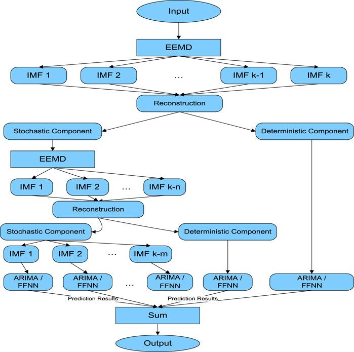
FIGURE 1. A flowchart of the proposed method.

2.1 ARIMA model

The ARIMA model is a type of stochastic process that can be used to analyze nonstationary time series. The autoregressive (AR), integrated (I), and moving average (MA) are the three major components of an ARIMA model. The future variable in an ARIMA model is meant to be a linear function of the past observations plus some random errors and p and q denote the model order. The random errors are assumed to be independent and distributed with a mean of zero and a standard deviation (SD) of σ2. It is also demonstrated as follows:

$y_t=\sigma +{\theta }_1{y}_{t-1}+{\theta }_2{y}_{t-2}+\dots \dots .+{\theta }_p{y}_{t-p}+{\phi }_1{q}_{t-1}+{\phi }_2{q}_{t-2}+\dots \dots .+{\phi }_p{q}_{t-q}(1)$

When p = 0, the model is also reduced to an MA model. Also, when the q = 0 model becomes an AR model non-stationary time series can be made stationary by differencing them once or twice. The Box and Jenkins methodology was used to select the best ARIMA model order. Model identification, parameter estimates, and diagnostic checking are the three primary steps of this process. The ACF and PACF of the time series are used in the “model identification” step to determine if the time series is stationary or non-stationary. To make non-stationary data stationary, the differencing operator is used one or more times to the time series. The second stage, parameter estimation, is simple after an appropriate ARIMA model has been selected. The model estimation error is decreased, and the optimal parameters are generated using some methods such as the least square estimate methodology. The Box–Jenkins model will examine whether the model error is satisfied in the final stage, called diagnostic checking. For this purpose, the L-Jung Box test was used in this work.

2.2 ANN model

Neural networks are parallel computing systems that seek to simulate the human brain on a computer. The main goal is to create a system that can execute various computer activities faster than traditional systems. ANN acquires a large number of units that are interconnected in some pattern to facilitate communication between the units. Basic parallel operating processors are often known as nodes or neurons. Every neuron is connected to other neurons via a connecting link. Each connection link has a weight that contains information about the input signal. Because the weight often excites or hinders the signal from being delivered, this is the most valuable knowledge for solving a specific problem for neurons. Each neuron has an internal state that is known as an activation signal. After the input signals and the activation rule have been combined, the output signals can be delivered to other units. The ANNs are used to model the nonlinear component of the Brent oil price in this research. Modeling of the nonlinear relationship between the input and output data-set is achievable with the help of ANNs. One of the most notable advantages of ANNs over other nonlinear modeling techniques is that they can be utilized as universal approximators to learn a wide number of functions accurately. The single hidden/middle layer ANN illustrated in Figure 2 is used.

FIGURE 2

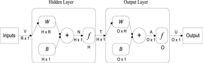
FIGURE 2. The general structure of ANN.

It's a three-layer feedforward multilayer perception (MLP): 1) input, 2) hidden, and 3) output. To model the time series, this paper uses a single-layer ANN. The following is a mathematical description of the relationship between the inputs and the output yt:

$y_t={\beta }_0+{\sum }_{j=1}^s{\beta }_j\mathrm{G}\left({\alpha }_{0j}+{\displaystyle \sum }_{i=1}^p{\alpha }_{ij}{y}_{t-i}\right)+{\alpha }_t(2)$

where p and s are the input and hidden layer node counts, where i = 1, 2..., p; j = 1, 2..., s, are the ANN biassing and weighting factors, respectively. G ( ) is also the ANN’s transfer function. The type of transfer function for the hidden layer in this study is a tangent-sigmoid function, which is defined as follows:

$f\left({\mathrm{Y}}_{\mathrm{t}}\right)=\frac{1}{1+e^{-Yt}}(3)$

exp () is the exponential operator, and y is the input vector. The ANN creates a nonlinear mapping between the input and output data as seen in Eq. 4:

$y_t=\left(y_{t-1},y_{t-2},\dots \dots ..,y_{t-p},\alpha ,\beta \right)+{\alpha }_t(4)$

where a and b are the biassing and weighting factors of the ANN’s vectors. According to recent studies, increasing the number of nodes (s) in the hidden layer of the simple ANN presented in Eq. 3 is a powerful model for learning nonlinear functions. However, a neural network with small nodes in the hidden layer is more powerful in out-of-sample forecasting. Indeed, as the number of nodes in the hidden layer grows, the ANN’s ability to fit nonlinear time series grows, but at the expense of the ANN’s ability to generalize out of the training data. This behavior can be interpreted as an overfitting event that occurs throughout the ANN modeling phase. An overfitted model can fit the data used as training data well, but it has a limited ability to generalize to samples outside of the training data.

2.3 Average mutual information

The IMFs are split into two parts, each of which requires a method or strategy that permits the deterministic and stochastic parts to be altered individually. From series to series, the cut-off points between two components of the examined sequence, such as stochastic and deterministic, differ. As a result, to estimate automatically, the RP (Kamphorst and Ruelle, 1987); and the mutual information (MI) (Shannon, 2001) these methods are commonly utilized. MI is employed to derive the stochastic and deterministic components in this study due to its simplicity and nonparametric behavior. The MI requirements were proposed by (Shannon, 2001).MI calculates shared data on the two variables related to the theory knowledge field. This term is explained via a simple demonstration. Because x1 does not have x2 knowledge (Kamphorst and Ruelle, 1987), let X1 and X2 be their MI = 0 random variables. In Eq. 5, the MI is shown between the two variables X1 and X2, where the joint density function of x1 and x2 is fx1fx2(x1,x2), and their marginal density functions are fx1 (x1) and fx2 (x2).

${\mathrm{M}\mathrm{I}}_{\left(\mathrm{X}1,\mathrm{X}2\right)}=\iint f_{X_{1,X_2}}\left(x_{1,}{x}_2\right)\mathit{log}\frac{f{X}_{1,}{X}_2\left(X_{1,}{X}_2\right)}{f{x}_{1,}\left(x_1\right).f{x}_2\left(X_2\right)}{d}_{x_1}{d}_{x_2}(5)$

The MI process is divided into three steps. To begin, divide the data into discrete, fixed-width cells (bins). In the second step, the focus is on frequencies to create a histogram for each cell (Ahmed and Shabri, 2014). In the third phase, the MI on each histogram is calculated. The IMF’s was broken down into two categories: stochastic and deterministic. The following is the equation that represents these elements

${\mathrm{S}\mathrm{C}}_{\left(\mathrm{t}\right)}={\displaystyle \sum }_{j=1}^k{IMF}_j\left(t\right)(6)$

${\mathrm{D}\mathrm{C}}_{\left(\mathrm{t}\right)}={\displaystyle \sum }_{j=k+1}^n{IMF}_j\left(\mathrm{t}\right)+\mathrm{r}\mathrm{e}\mathrm{s}\mathrm{i}\mathrm{d}\mathrm{u}\mathrm{e}(7)$

Where DC is the deterministic component, SC is the stochastic component, k is the number of stochastic IMFs, and n is the overall number of IMFs. The EEMD approach guarantees that the sum of all IMFs and residues will produce the original time series. As a result, we may restore the original series by combining the stochastic and deterministic components.

2.4 EMD

The EMD is a technique for nonlinear signal modification that was developed by (Huang et al., 1999a). This method is used to transform nonlinear and nonstationary time series data into intrinsic mode functions (IMFs) having a single intrinsic time measure property. According to (Huang et al., 1999a), each IMF must meet both conditions. The number of extreme and zero crossings’ values must be identical or differ by no more than one value, and the average value of the envelope must be zero at any site formed by local minima and maxima. The decomposition procedure of a time series data is as follows:

i) Detect all local minima and maxima of the series $Y_t.$

ii) Compute the lower envelope $Y_t\left(l\right)$ and upper envelope $Y_t\left(u\right)$ for the series $Y_t.$

iii) Use the lower and upper envelope to obtain the first mean time series $m_t\left(\mathit{1}\right)$, i.e., $m_t\left(\mathit{1}\right)=\left(Y_t\left(l\right)+Y_t\left(u\right)\right)/\mathit{2}$.

iv) To get the first IMF ${imf}_t\left(\mathit{1}\right)$, find the difference between the series $Y_t$ and the mean series $m_t\left(\mathit{1}\right)$. i.e., ${imf}_t\left(\mathit{1}\right)=Y_t-m_t\left(\mathit{1}\right)$. Furthermore, the two conditions will be checked for ${imf}_t\left(\mathit{1}\right)$, if it does not satisfy both conditions, then steps (i) to (iii) of the decomposition process will be repeated to obtain the first IMF.

v) Repeat the above steps to get all IMFs, until the final residue ${resid}_t$, which is a monotonic function proposed for the discontinuing of the decomposition process (Huang et al., 1999b).

To get back the original time series $x_t$ from the IMFs and residue simply add these components using this equation. $Y_t={\displaystyle \sum }_i^n{imf}_t\left(i\right)+{resid}_t$, where n is the total number of IMFs. The sifting process stops when the residual $r_t$ becomes a monotonic function.

2.5 EEMD

Wu and Huang (2009) presented the Ensemble Empirical Mode Decomposition (EEMD) to discuss the mode mixing problem in EMD. As a result of mode mixing, the IMF component takes on distinct timeframe characteristics and evolves into a scale-dependent oscillation, losing its original physical significance. Several white noises are added to the original time series, and because the frequency of these white noises is greatly dependent on EEMD, 0.20 was applied to the daily Brent oil prices series by default (Aamir and Shabri, 2018). The algorithm flow of EEMD is as follows:

i) Introduce several Gaussian white noises $x_t\left(i\right)$ into crude oil price $Y_t$, $x_t\left(i\right)\sim N\left(\mathit{0},{\sigma }^{\mathit{2}}\right)$.

$Y_t\left(i\right)=Y_t+x_t\left(i\right)$

ii) Conduct the EMD decomposition on $Y_t\left(i\right)$ respectively and obtaining a set of IMFs ${imf}_t\left(ij\right)$ and a residue ${resid}_t\left(i\right)$, where ${imf}_t\left(ij\right)$ is the $j^{th}$ IMF decomposed by EMD after adding the Gaussian white noise for an $i^{th}$ time.

iii) Repeat the above-mentioned steps. The ensemble average of corresponding IMFs is seen as the final decomposition result.

${imf}_t\left(i\right)=\frac{1}{N}{\displaystyle \sum }_{j=1}^N{imf}_t\left(ij\right)$

where $N$ is the ensemble size.

The EEMD can effectively solve the mode mixing existing problem in the traditional EMD. As a result, the decomposition becomes more stable and physically meaningful.

2.6 EEMD-ARIMA/FFNN

All of the IMFs obtained from EEMD are used in the EEMD-ARIMA model. This approach is also known as the RDE model (reconstruction decomposition ensemble). All IMFs are modeled and used for predicting in this technique. The EEMD-ARIMA technique can be broken down into three simple parts.

i) EEMD decomposed the original time series into n components IMFs.

ii) For all of the extracted IMFs, the best ARIMA model is chosen, and the respective series are modeled and predicted appropriately.

iii) Finally, all IMFs’ anticipated results are added together, and the output of the targeted time series is obtained. The goal of decomposition is to make forecasting easier, but the goal of the ensemble is to reformulate the decomposed component into a single series that can be used to forecast the original data.

2.7 EEMD-SD-ARIMA/FFNN

To begin, visually evaluate AMI graphs to divide EEMD-ARIMA model components into two parts: stochastic and deterministic components. Individual stochastic and one deterministic component is used in the EEMD-SD-ARIMA/FFNN model. Finally, MAE, MAPE, and RMSE were used to test the accuracy of this hybrid model. The complete process of reconstruction of IMFs obtained from EEMD is as follows:

i) Apply the EEMD technique to the original time series $Y_t$ to gather all IMFs.

ii) Compute different characteristics of all IMFs e.g., Average mutual information (AMI), recurrence plot, autocorrelation.

iii) Based on each IMF characteristic divide the IMFs into components according to their nature like stochastic or deterministic.

Reconstruction is complete and applies the different models to the new form components.

2.8 EEMD-S2-ARIMA/FFNN

The suggested method starts by adding the stochastic IMFs of the hybrid model EEMD-SD-ARIMA/FFNN as a single component and then applying EEMD to it. As a result, numerous IMFs were generated, and ARIMA/FFNN models were fitted to each of the IMFs in the hybrid model EEMD-S2-ARIMA/FFNN. Because stochastic IMFs do not correlate with their previous lags, and since forecasting requires that the current value correlates with its past value, this suggests that there is some unneeded noise present in these stochastic IMFs, which needs to be divided further.

2.9 EEMD-SD1D2-ARIMA/FFNN

Individual stochastic and deterministic components make up the EEMD-SD1D2-ARIMA model. Finally, individual stochastic and two deterministic components were subjected to ARIMA and FFNN models, and the prediction accuracy of the proposed EEMD-SD1D2-ARIMA/FFNN hybrid model was assessed using MAE, RMSE, and MAPE.

2.10 EEMD-S + D1+D2-ARIMA/FFNN

The hybrid model EEMD-S + D1+D2-ARIMA combines stochastic and deterministic components. FFNN and ARIMA models were used to test the correctness of this hybrid model. In this model, the stochastic component and deterministic component in the second stage, and the deterministic component in the first stage were used to forecast the crude oil prices.

3 Analysis

3.1 Simulation study

For simulation, a time series was created using a sine function, a third-order autoregressive model, and a normal distribution. The sine function with an angular frequency of 2$\pi$ was used to create a deterministic component, while the AR(3) and N functions were used to create a stochastic component using AR(3) and N (0,1). The results were validated with various numbers of observations, including N = 50, 500, 1,000, 2000, 5,000, and 7,500. As a result, the noisy time series was created by combining all of the components (Xu et al., 2020; Ahmad et al., 2021).

$\mathrm{Y}\mathrm{t}=\sin \left(2\pi \right)+\mathrm{A}\mathrm{R}\left(3\right)+\mathrm{N}\left(\mathrm{0,1}\right)(8)$

To divide the IMFs into stochastic and deterministic components the AMI plots are used. For various numbers of observations i.e., N = 50, 500, 1,000, 2000, 5,000, and 7,500 the AMI plots are presented in the following figures respectively. The order of ARIMA models are presented in Table 1 for all IMFs of different sample sizes of simulation study. Secondly, the LB test values are presented in Table 2.

TABLE 1

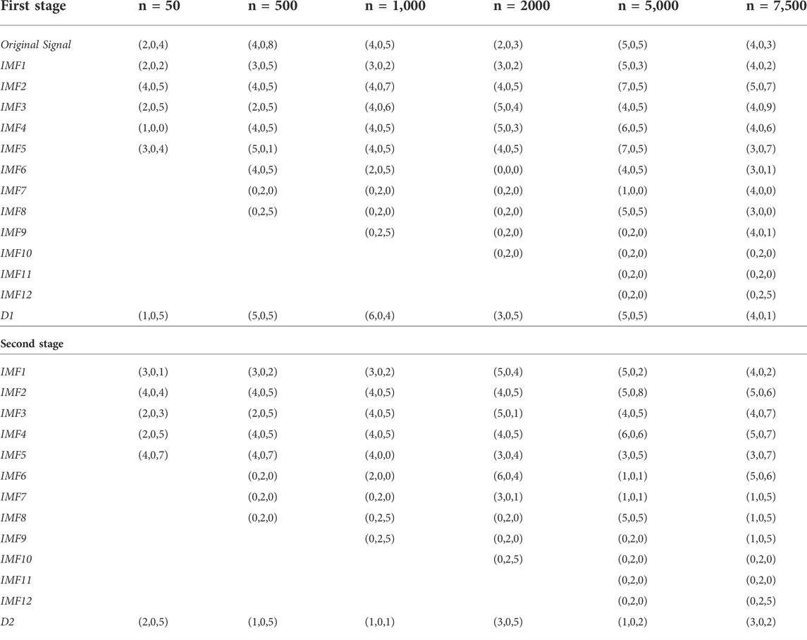
TABLE 1. The order of the ARIMA models.

TABLE 2

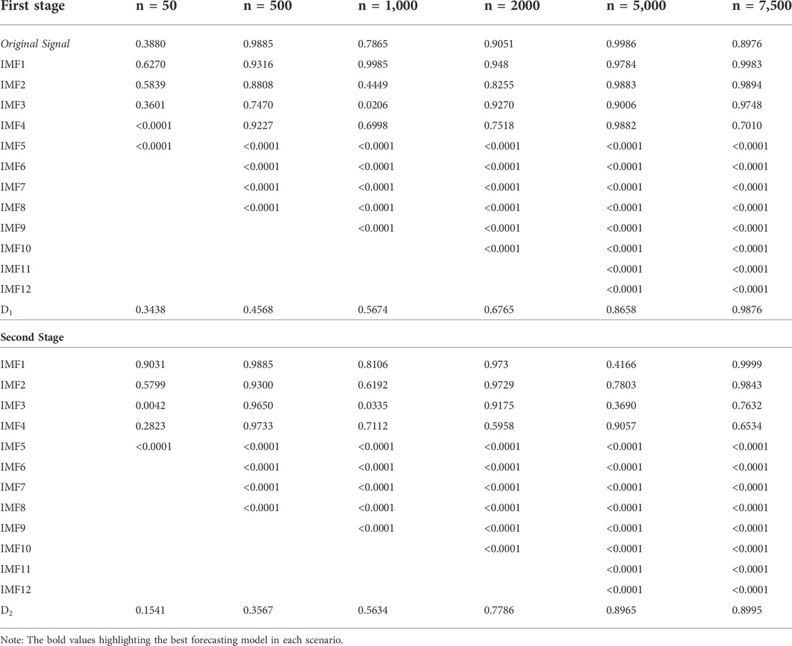
TABLE 2. L-Jung Box test p-values of ARIMA and EEMD-ARIMA models at the first stage.

After observing above Figure 3, the first three IMFs were taken as stochastic and the last two components as deterministic. Also, from Figure 4 the first four IMFs, from Figures 5, 6 the first six IMFs, and in Figures 7-9 the first seven IMFs were taken as stochastic, and the rest of the IMFs were reserved as deterministic respectively.

FIGURE 3

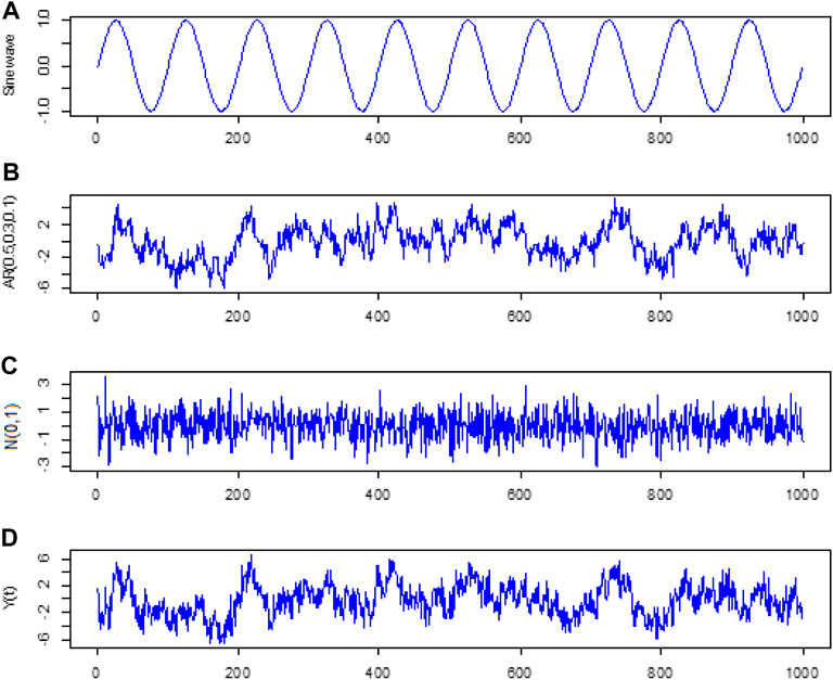
FIGURE 3. (A) Deterministic component $\left(\mathit{2}\pi t\right)$ , (B) Stochastic component $AR\left(\mathit{3}\right)$ (C) white noise $N\left(\mathit{0,1}\right)$ (D) The noisy time series $Y_t=\mathit{Sin}\left(\mathit{2}\pi t\right)+AR\left(\mathit{3}\right)+N\left(\mathit{0,1}\right)$.

FIGURE 4

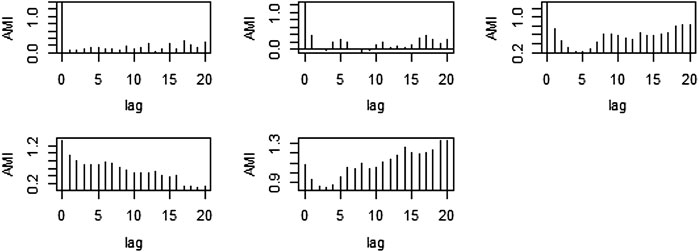
FIGURE 4. AMI graph of the proposed method for N = 50.

FIGURE 5

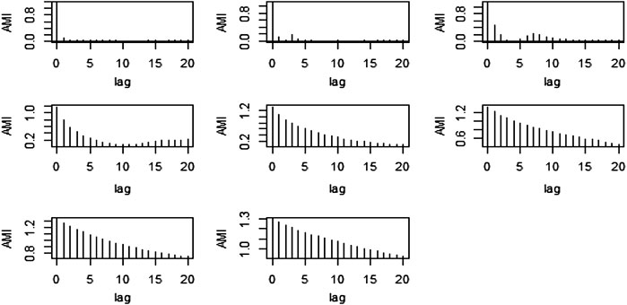
FIGURE 5. AMI graph of the proposed method for N = 500.

FIGURE 6

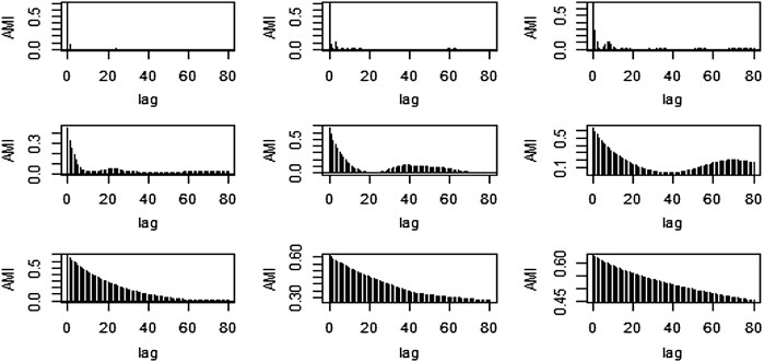
FIGURE 6. AMI graph of the proposed method for N = 1,000.

FIGURE 7

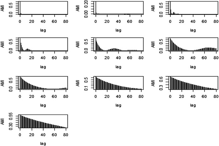
FIGURE 7. AMI graph of the proposed method for N = 2000.

FIGURE 8

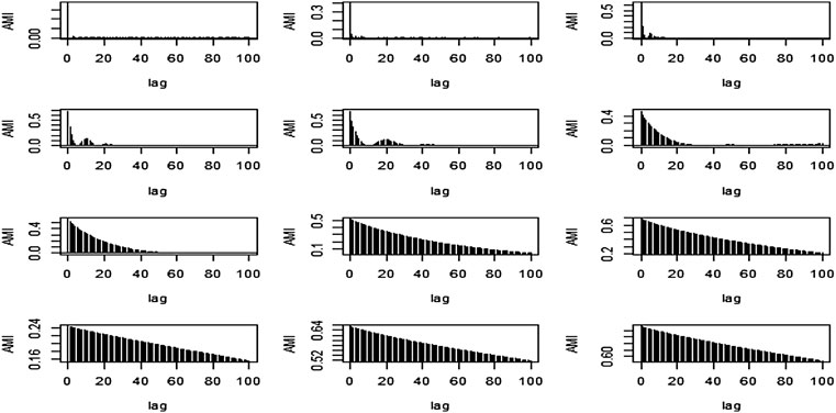
FIGURE 8. AMI graph of the proposed method for N = 5,000.

FIGURE 9

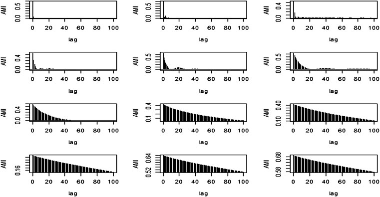
FIGURE 9. AMI graph of the proposed method for N = 7,500.

3.2 Diagnostic checking

For diagnostic checking, the statistical test is used which may infer a denial of the fitted model. The test to be used is the Ljung-Box (LB), which tests the serials independence among the fitted model residual. The first step in this test is the extraction of the fitted model residuals. The extracted T residuals from the fitted model are used to attain the sample autocorrelations using the subsequent formulation:

${\widehat{r}}_{\kappa }=\frac{{\sum }_{t=\kappa +1}^T{\widehat{ϵ}}_t{\widehat{ϵ}}_{t-\kappa }}{{\displaystyle \sum }_{t=1}^T{\widehat{ϵ}}_t^2},\kappa =\mathrm{1,2},\dots (9)$

The autocorrelations obtained from Eq. 9 are then tested for serial dependence using the LB test. Eq. 10 is used for the said purpose of testing the hypothesis of independence against the serially dependent hypothesis. The LB test test-statistic is as follows:

$\stackrel{\sim }{Q}\left(r\right)=T\left(T+2\right){\displaystyle \sum }_{\kappa =1}^n{\left(T-\kappa \right)}^{-1}{r}_{\kappa }^2(10)$

The Q(r) statistic is distributed asymptotically as an X ∼ a(n), where a is the significance level and n is the degrees of freedom and number of lagged autocorrelations.

LB test was applied to check the model adequacy for n = 50, 500, 1,000, 2000, 5,000, and 7,500 for a 5% level of significance under the null hypothesis that the series is stationary. The p-value of 0.0001 shows that the series is not stationary and vice versa.

A simulation study was performed to check the adequacy of the proposed method for different sample sizes. Hybrid model EEMD-S1-ARIMA outperformed the other hybrid models for n = 50 and 500. However, in other cases, for n = 1,000, 2000, 5,000, and 7,500, the proposed hybrid model EEMD-S2D1D2-ARIMA performed well. This shows that the sample size has a greater impact on the performance of the proposed hybrid model because for a small sample EEMD generated a smaller number of IMFs and has more stochasticity present in between them due to this reason, the proposed hybrid model EEMD-S1-ARIMA performed well because in this model all IMFs were modeled individually. As the sample size increases, EEMD components have high variability present in them that’s why the reconstruction of IMFs at the second stage was performed to reduce the variability that is present between them. The proposed hybrid model EEMD-S2D1D2-ARIMA has minimum MAE, RMSE, and MAPE for N = 1,000, 2000, 5000, and 7,500. Figures 10, 11 showing the forecasting performance of the used hybrid models which confirms the superiority of the proposed method.

FIGURE 10

FIGURE 10. Accuracy measures graph of simulation study for n = 50, 500, 1,000, 2000, 5,000, and 7,500.

FIGURE 11

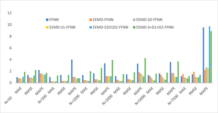
FIGURE 11. Accuracy measures of FFNN hybrid models.

FFNN model was also applied to check the performance of the proposed method. The hybrid model EEMD-S1-FFNN outperformed the other hybrid model for N = 50 and 500, which shows that this hybrid model is good for a small sample size. On the other hand, EEMD-S2D1D2-FFNN worked well, and it showed minimum MAE, RMSE, and MAPE to other hybrid models. The forecasting accuracy measures for both ARIMA and FFNN hybrid models are presented in Tables 3, 4.

TABLE 3

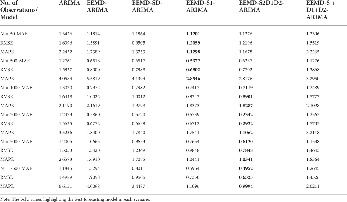
TABLE 3. Accuracy measures of the proposed hybrid model using ARIMA.

TABLE 4

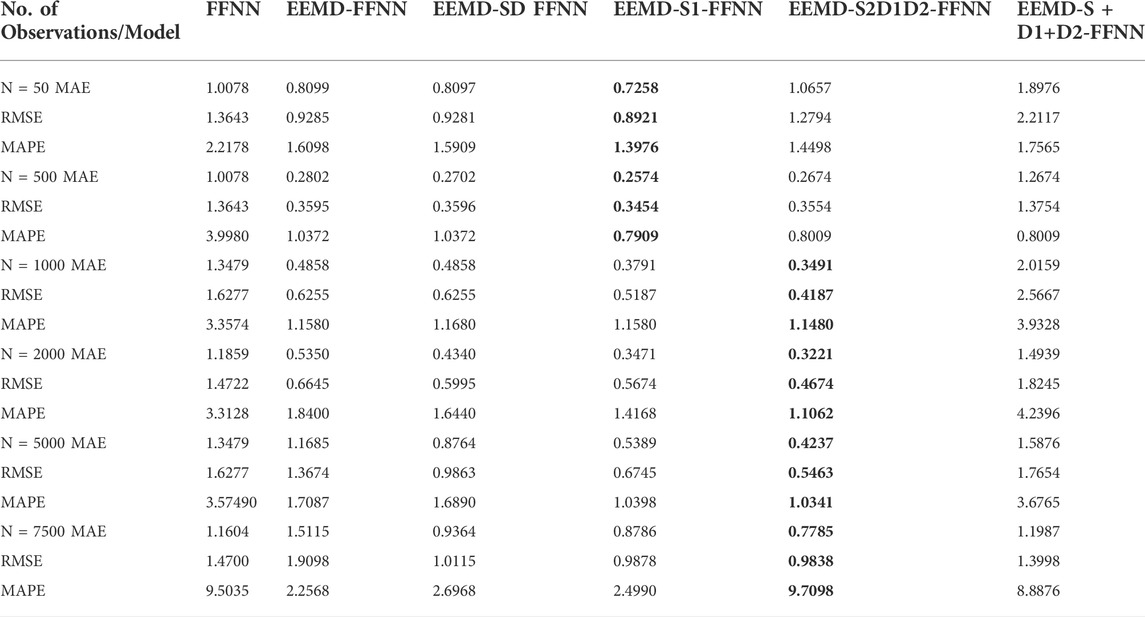
TABLE 4. Accuracy measures of the proposed hybrid models using FFNN.

3.3 Data description

The data used in this study were daily Brent crude oil prices. This data was divided into two sets 80% training and 20% testing (Ahmed and Shabri, 2014; Aamir et al., 2018). The Brent oil prices was consisting of 4,933 observations and presented in Figure 12. From the graph of the Brent crude oil prices, it is observed that there are no trend, seasonal, or cyclic variations but irregular variations.

FIGURE 12

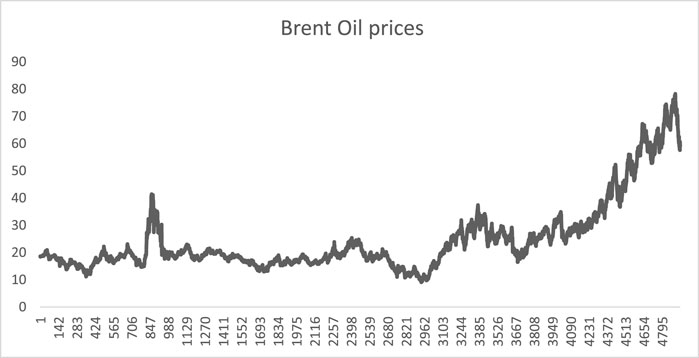
FIGURE 12. Daily Brent crude oil prices data.

To check the stationarity of a series ADF test was applied to the training set of the data. The p-value of the ADF test was 0.04776. FFNN was also applied to the data and the number of lags was chosen according to the auto-regressive term of the ARIMA model and hidden layers were chosen according to formula (2×k+1) (AAMIR, 2018). The EEMD was presented by (Wu and Huang, 2009) to discourse on the mode mixing problem of EMD. The consequence of mode mixing is that the IMF component will consist of different timescale characteristics and becomes scale-dependent oscillation and therefore losses its original physical meaning. Several white noises are added to the original time series EEMD highly depends on the frequency of these white noises so by default 0.20 is used. The graphs of the decomposed series are presented in Figure 13.

FIGURE 13

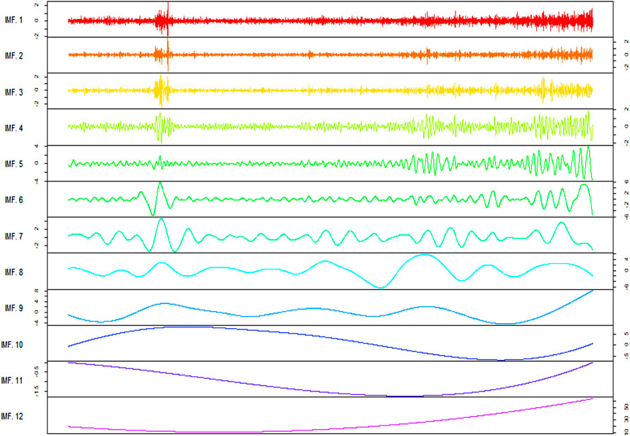
FIGURE 13. Brent Oil prices IMFs generated by EEMD.

The order of the selected ARIMA models for all IMFs with their respective values of the LB test is presented in Table 5,6.

TABLE 5

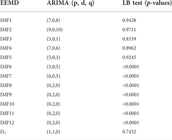
TABLE 5. Order of ARIMA model of Gao et al. (2019) method.

TABLE 6

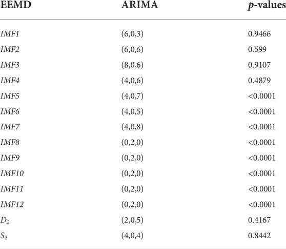
TABLE 6. Order of ARIMA model and LB test p-values.

3.4 AMI plots

The method used for comparison is based on the reconstruction of IMFs via AMI plots. The plots of the AMI are presented in Figure 14.

FIGURE 14

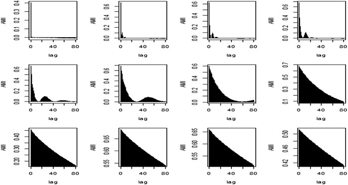
FIGURE 14. AMI graphs of Gao et al. (2019) method.

By the visual inspection of the AMI graphs, the first 7 IMFs were considered Stochastic, and the rest of the IMFs were added and considered Deterministic components. Since all of these 7 IMFs follow a different trend, the IMFs from 1 to 7 follow a stochastic pattern, showing that there are no dependencies of upcoming observations on past observations. This can also be proven by the MAE, RMSE, and MAPE of the stochastic and deterministic components which are (0.7879, 1.0342, and 115.3129) and (0.0001, 0.0013, and 0.0005) respectively. So, from these measures, it was concluded that the stochastic component has more variation, and they should be modeled individually.

3.5 The proposed method

The stochastic components of the comparison method were added as a single stochastic component and then EEMD was applied to that stochastic component. The plot of the stochastic component IMFs of the second stage of EEMD is presented in Figure 15.

FIGURE 15

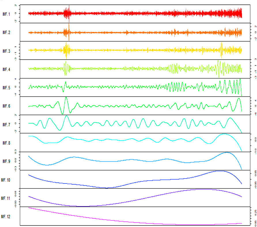
FIGURE 15. Stochastic component and IMFs of the second stage EEMD.

Reconstruction of IMFs was performed again by the visual inspection of the AMI plots at the second stage and the plots are as under:

Based on Figure 16 the IMFs were divided into Stochastic and Deterministic components. Our focus is on the Stochastic component because it contributes more variation as compared to the Deterministic component. The Stochastic component consists of the first six IMFs while the rest of the IMFs were considered Deterministic. The order of the ARIMA model of Stochastic component are as follows.

FIGURE 16

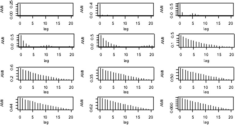
FIGURE 16. AMI graphs of the proposed method.

The forecasting accuracy measures of all the models for Brent crude oil prices data are presented in Table 7 and for more clearer picture plotted in Figure 17. The values of the best forecasting accuracy models are highlighted.

TABLE 7

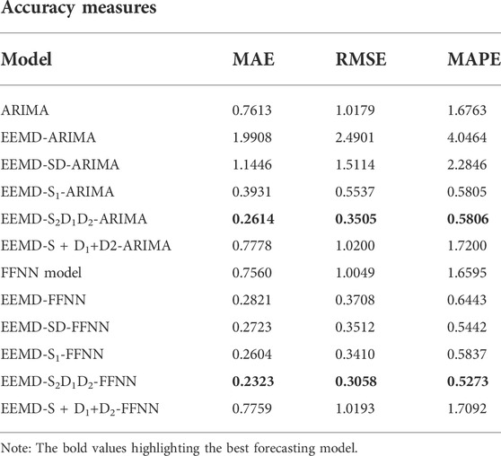
TABLE 7. Comparison of results of the proposed model and interpretable benchmark models.

FIGURE 17

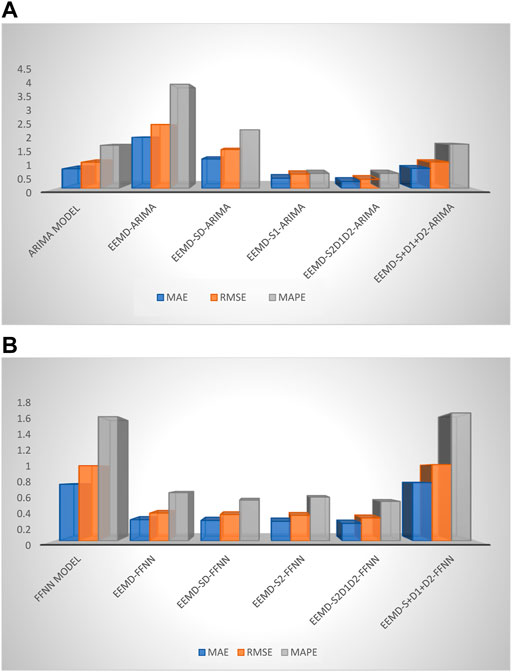
FIGURE 17. Plot of the accuracy measures based on (A) ARIMA and (B) FFNN models.

3.6 Discussion

In this study, three hybrid models were proposed and compared with the existing method of reconstruction of IMFs. EEMD components were reconstructed at two stages, in earlier studies EEMD components were reconstructed at only one stage but a novel method was proposed in which EEMD components were reconstructed at two stages through AMI graphs. A simulation study was performed to check the adequacy of the proposed method for N = 50, 500, 1,000, 2000, 5,000, and 7,500. EEMD generates a different number of IMFs for different sample sizes. The hybrid model EEMD-S1-ARIMA performed well for N = 50 and 500 as compared to the existing and the other two proposed hybrid models, similarly EEMD-S2D1D2-ARIMA/FFNN hybrid model outperformed the other models for N = 1,000, 2000, 5,000, and 7,500, with minimum MAE, RMSE, and MAPE.

Apart from the simulation study, Brent crude oil prices data was also used to check the performance of the proposed hybrid model, which also showed higher efficiency as compared to other hybrid models that have been used in this study. Based on forecasting accuracy measures the proposed hybrid model EEMD-S₂D₁D₂-ARIMA/FFNN outperformed its counterpart models. Both models i.e., EEMD-S₂D₁D₂-ARIMA and EEMD-S₂D₁D₂-ARIMA/FFNN performed well when used in the proposed scenario. The MAPE values of EEMD-S₂D₁D₂-ARIMA and EEMD-S₂D₁D₂-ARIMA/FFNN are 0.5806 and 0.5273 respectively, which is less than 1 indicating that the proposed models fall in the range of perfect models (Aamir and Shabri, 2018). Hence it was concluded that the proposed hybrid model EEMD-S2D1D2-ARIMA/FFNN has a significant capability to predict the crude oil prices as compared to the rest of the hybrid models.

From the above discussions and analysis, some important findings are summarized as follows:

i) To accurately forecast the crude oil prices, it is hard to attain satisfactory results when using single models (i.e., FFNN and ARIMA) due to the nonlinearity and nonstationary structure of the data.

ii) The models which used all decomposed IMFs relatively performed well than the models which used the reconstructed IMFs only in two components i.e., deterministic, and stochastic.

iii) Based on the synthetic data the proposed method of reconstruction of IMFs at two stages proved that the reconstruction of IMFs through AMI is a better and simple strategy that enhanced the performance of both models i.e., ARIMA and FFNN.

iv) With the benefits of EEMD, reconstruction, ARIMA, and FFNN, the proposed ensemble models EEMD-S2D1D2-ARIMA and EEMD-S2D1D2-FFNN significantly outperform all other models listed in this study in terms of MAPE, RMSE, and MAE.

v) The performance of the proposed models EEMD-S2D1D2-ARIMA and EEMD-S2D1D2-FFNN are almost the same. However, in terms of MAPE, RMSE, and MAE the model EEMD-S2D1D2-FFNN relatively performed well compared to EEMD-S2D1D2-ARIMA. Therefore, the suggested model for forecasting crude oil prices is EEMD-S2D1D2-FFNN.

vi) The experimental results demonstrated that the reconstruction of IMFs into stochastic and deterministic components using the proposed method was effective but modeling the IMFs being part of the stochastic component separately was the more effective and powerful approach for forecasting crude oil prices.

vii) As one of the most important commodities in the world, we analyze the COPs for illustration and verification of the proposed method. *e empirical results showed that our proposed reconstruction of decomposition and ensemble model-based analysis approach is vital and effective and could be tested for more complex tasks.

4 Conclusion

The price of crude oil, known as the lifeblood of the global industry, has an important influence on practitioners, scholars, and politicians. Therefore, a stable, and reliable prediction of crude oil prices are helpful for national security and economic development, enterprise operations, and investment. However, crude oil prices are extremely unstable, and some traditional point forecasting methods no longer work, against the background of the Russia-Ukraine war and COVID-19.

In this study, a new hybrid model for the forecasting of crude oil prices is proposed. Considering the shortcomings of existing data decomposition and reconstruction of decomposition techniques, we propose a new reconstruction of data decomposition technique work in two steps, which can differentiate components based on stochastic and deterministic influences. Then, In the first step, we distinguish and reconstruct components with their influences. In the next step retain the deterministic and again apply EEMD on the stochastic component. Based on AMIs split the IMFs into two components i.e., stochastic, and deterministic. The ARIMA and FFNN models were applied to the reconstructed components to model the crude oil prices. After predicting the different components separately for the final output all the results are simply added. Finally, the point forecast based on ARIMA and FFNN models was obtained. Comparisons with various benchmark models show that the proposed reconstruction of IMFs has improved forecasting performance for both ARIMA and FFNN models. Furthermore, due to the excellent and stable prediction ability of the proposed reconstruction of IMFs method, we believe that it is also suitable for prediction tasks in other domains.

Although our developed system has achieved good results, there is still room for improvement. Our future research work is based on the following two aspects:

i) At present, many new techniques for the reconstruction of IMFs have been proposed, such as autocorrelation, low, medium, and high frequencies, stationarity, ARIMA model, etc. We hope to introduce advanced techniques to further enhance the forecasting performance and simplify the model.

ii) As the crude oil price fluctuates greatly at present, we consider establishing an early warning system for price mutation in the future.

Data availability statement

Datasets were analyzed in this study are included in the article/Supplementary Material, further inquiries can be directed to the corresponding authors.

Author contributions

All authors listed have made a substantial, direct, and intellectual contribution to the work and approved it for publication.

Conflict of interest

The authors declare that the research was conducted in the absence of any commercial or financial relationships that could be construed as a potential conflict of interest.

Publisher’s note

All claims expressed in this article are solely those of the authors and do not necessarily represent those of their affiliated organizations, or those of the publisher, the editors and the reviewers. Any product that may be evaluated in this article, or claim that may be made by its manufacturer, is not guaranteed or endorsed by the publisher.

References

Aamir, M. (2018). Crude oil price forecasting based on the reconstruction of imfs of decomposition ensemble model with arima and ffnn models. PhD thesis (Johor Bahru, Malaysia: Universiti Teknologi Malaysia).

Aamir, M., and Shabri, A. (2018). Improving crude oil price forecasting accuracy via decomposition and ensemble model by reconstructing the stochastic and deterministic influences. Adv. Sci. Lett. 24, 4337–4342. doi:10.1166/asl.2018.11601

CrossRef Full Text | Google Scholar

Aamir, M., Shabri, A., and Ishaq, M. (2018). Improving forecasting accuracy of crude oil prices using decomposition ensemble model with reconstruction of IMFs based on ARIMA model. Mal. J. Fund. Appl. Sci. 14, 471–483. doi:10.11113/mjfas.v14n4.1013

CrossRef Full Text | Google Scholar

Ahmad, W., Aamir, M., Khalil, U., Ishaq, M., Iqbal, N., and Khan, M. (2021). A new approach for forecasting crude oil prices using median ensemble empirical mode decomposition and group method of data handling. Math. Problems Eng. 2021, 1–12. doi:10.1155/2021/5589717

CrossRef Full Text | Google Scholar

Ahmed, R. A., and Shabri, A. B. (2014). Daily crude oil price forecasting model using arima, generalized autoregressive conditional heteroscedastic and support vector machines. Am. J. Appl. Sci. 11, 425–432. doi:10.3844/ajassp.2014.425.432

CrossRef Full Text | Google Scholar

Cicone, A., and Zhou, H. (2021). Numerical analysis for iterative filtering with new efficient implementations based on FFT. Numer. Math. (Heidelb). 147, 1–28. doi:10.1007/s00211-020-01165-5

CrossRef Full Text | Google Scholar

Gao, W., Aamir, M., Shabri, A. B., Dewan, R., and Aslam, A. (2019). Forecasting crude oil price using kalman filter based on the reconstruction of modes of decomposition ensemble model. IEEE Access 7, 149908–149925. doi:10.1109/access.2019.2946992

CrossRef Full Text | Google Scholar

He, K., and Zou, Y. (2022). Crude oil risk forecasting using mode decomposition based model. Procedia Comput. Sci. 199, 309–314. doi:10.1016/j.procs.2022.01.038

CrossRef Full Text | Google Scholar

Huang, N. E., Shen, Z., and Long, S. R. (1999a). A new view of nonlinear water waves: The hilbert spectrum. Annu. Rev. Fluid Mech. 31, 417–457. doi:10.1146/annurev.fluid.31.1.417

CrossRef Full Text | Google Scholar

Huang, N. E., Shen, Z., and Long, S. R. (1999b). A new view of nonlinear water waves: The hilbert spectrum. Annu. Rev. Fluid Mech. 31, 417–457. doi:10.1146/annurev.fluid.31.1.417

CrossRef Full Text | Google Scholar

Huang, N. E., Wu, M. L. C., Long, S. R., Shen, S. S., Qu, W., Gloersen, P., et al. (2003). A confidence limit for the empirical mode decomposition and Hilbert spectral analysis. Proc. R. Soc. Lond. A 459, 2317–2345. doi:10.1098/rspa.2003.1123

CrossRef Full Text | Google Scholar

Jammazi, R., and Aloui, C. (2012). Crude oil price forecasting: Experimental evidence from wavelet decomposition and neural network modeling. Energy Econ. 34, 828–841. doi:10.1016/j.eneco.2011.07.018

CrossRef Full Text | Google Scholar

Kamdem, J. S., Essomba, R. B., and Berinyuy, J. N. (2020). Deep learning models for forecasting and analyzing the implications of COVID-19 spread on some commodities markets volatilities. Chaos, Solit. Fractals 140, 110215. doi:10.1016/j.chaos.2020.110215

CrossRef Full Text | Google Scholar

Kamphorst, J. P. E. S. O., and Ruelle, D. (1987). Recurrence plots of dynamical systems. Europhys. Lett. 4, 973–977. doi:10.1209/0295-5075/4/9/004

CrossRef Full Text | Google Scholar

Karasu, S., Altan, A., Bekiros, S., and Ahmad, W. (2020). A new forecasting model with wrapper-based feature selection approach using multi-objective optimization technique for chaotic crude oil time series. Energy 212, 118750. doi:10.1016/j.energy.2020.118750

CrossRef Full Text | Google Scholar

Kilian, L., and Murphy, D. P. (2014). The role of inventories and speculative trading in the global market for crude oil. J. Appl. Econ. Chichester. Engl. 29, 454–478. doi:10.1002/jae.2322

CrossRef Full Text | Google Scholar

Kilian, L. (2009). Not all oil price shocks are alike: Disentangling demand and supply shocks in the crude oil market. Am. Econ. Rev. 99, 1053–1069. doi:10.1257/aer.99.3.1053

CrossRef Full Text | Google Scholar

Li, G., Yin, S., and Yang, H. (2022). A novel crude oil prices forecasting model based on secondary decomposition. Energy 257, 124684. doi:10.1016/j.energy.2022.124684

CrossRef Full Text | Google Scholar

Li, T., Zhou, M., Guo, C., Luo, M., Wu, J., Pan, F., et al. (2016). Forecasting crude oil price using EEMD and RVM with adaptive PSO-based kernels. Energies 9, 1014. doi:10.3390/en9121014

CrossRef Full Text | Google Scholar

Lin, H., and Sun, Q. (2020). Crude oil prices forecasting: An approach of using CEEMDAN-based multi-layer gated recurrent unit networks. Energies 13, 1543. doi:10.3390/en13071543

CrossRef Full Text | Google Scholar

Lizardo, R. A., and Mollick, A. V. (2010). Oil price fluctuations and US dollar exchange rates. Energy Econ. 32, 399–408. doi:10.1016/j.eneco.2009.10.005

CrossRef Full Text | Google Scholar

Moshiri, S., and Foroutan, F. (2006). Forecasting nonlinear crude oil futures prices. energy J. 27. doi:10.5547/issn0195-6574-ej-vol27-no4-4

CrossRef Full Text | Google Scholar

Mostafa, M. M., and El-Masry, A. A. (2016). Oil price forecasting using gene expression programming and artificial neural networks. Econ. Model. 54, 40–53. doi:10.1016/j.econmod.2015.12.014

CrossRef Full Text | Google Scholar

Movagharnejad, K., Mehdizadeh, B., Banihashemi, M., and Kordkheili, M. S. (2011). Forecasting the differences between various commercial oil prices in the Persian Gulf region by neural network. Energy 36, 3979–3984. doi:10.1016/j.energy.2011.05.004

CrossRef Full Text | Google Scholar

Nademi, A., and Nademi, Y. (2018). Forecasting crude oil prices by a semiparametric Markov switching model: OPEC, WTI, and brent cases. Energy Econ. 74, 757–766. doi:10.1016/j.eneco.2018.06.020

CrossRef Full Text | Google Scholar

Piersanti, G., Piersanti, M., Cicone, A., Canofari, P., and Di Domizio, M. (2020). An inquiry into the structure and dynamics of crude oil price using the fast iterative filtering algorithm. Energy Econ. 92, 104952. doi:10.1016/j.eneco.2020.104952

CrossRef Full Text | Google Scholar

Sahir, M. H., and Qureshi, A. H. (2007). Specific concerns of Pakistan in the context of energy security issues and geopolitics of the region. Energy policy 35, 2031–2037. doi:10.1016/j.enpol.2006.08.010

CrossRef Full Text | Google Scholar

Shannon, C. E. (2001). A mathematical theory of communication. Sigmob. Mob. Comput. Commun. Rev. 5, 3–55. doi:10.1145/584091.584093

CrossRef Full Text | Google Scholar

Sun, J., Zhao, P., and Sun, S. (2022). A new secondary decomposition-reconstruction-ensemble approach for crude oil price forecasting. Resour. Policy 77, 102762. doi:10.1016/j.resourpol.2022.102762

CrossRef Full Text | Google Scholar

Wu, C., Wang, J., and Hao, Y. (2022). Deterministic and uncertainty crude oil price forecasting based on outlier detection and modified multi-objective optimization algorithm. Resour. Policy 77, 102780. doi:10.1016/j.resourpol.2022.102780

CrossRef Full Text | Google Scholar

Wu, Y. X., Wu, Q. B., and Zhu, J. Q. (2019). Improved EEMD-based crude oil price forecasting using LSTM networks. Phys. A Stat. Mech. its Appl. 516, 114–124. doi:10.1016/j.physa.2018.09.120

CrossRef Full Text | Google Scholar

Wu, Z., and Huang, N. E. (2009). Ensemble empirical mode decomposition: A noise-assisted data analysis method. Adv. Adapt. Data Anal. 1, 1–41. doi:10.1142/s1793536909000047

CrossRef Full Text | Google Scholar

Xiang, Y., and Zhuang, X. H. (2013). “Application of ARIMA model in short-term prediction of international crude oil price,” in Advanced materials research (Stafa-Zurich, Switzerland: Trans Tech Publ), 979–982.

CrossRef Full Text | Google Scholar

Xie, W., Yu, L., Xu, S., and Wang, S. (2006). “A new method for crude oil price forecasting based on support vector machines,” in Computational science–ICCS 2006 (Berlin, Germany: Springer), 444–451.

CrossRef Full Text | Google Scholar

Xiong, T., Bao, Y., and Hu, Z. (2013). This is a preprint copy that has been accepted for publication in Knowledge-based Systems.

Google Scholar

Xu, P., Aamir, M., Shabri, A., Ishaq, M., Aslam, A., and Li, L. (2020). A new approach for reconstruction of IMFs of decomposition and ensemble model for forecasting crude oil prices. Math. Problems Eng. 2020, 1–23. doi:10.1155/2020/1325071

CrossRef Full Text | Google Scholar

Yu, L., Dai, W., and Tang, L. (2016). A novel decomposition ensemble model with extended extreme learning machine for crude oil price forecasting. Eng. Appl. Artif. Intell. 47, 110–121. doi:10.1016/j.engappai.2015.04.016

CrossRef Full Text | Google Scholar

Yu, L., Wang, S., and Lai, K. K. (2008). Forecasting crude oil price with an EMD-based neural network ensemble learning paradigm. Energy Econ. 30, 2623–2635. doi:10.1016/j.eneco.2008.05.003

CrossRef Full Text | Google Scholar

Yu, L., Wang, Z., and Tang, L. (2015). A decomposition–ensemble model with data-characteristic-driven reconstruction for crude oil price forecasting. Appl. Energy 156, 251–267. doi:10.1016/j.apenergy.2015.07.025

CrossRef Full Text | Google Scholar

Yu, L., Zhao, Y., and Tang, L. (2014). A compressed sensing based AI learning paradigm for crude oil price forecasting. Energy Econ. 46, 236–245. doi:10.1016/j.eneco.2014.09.019

CrossRef Full Text | Google Scholar

Yusof, Y., and Mustaffa, Z. (2016). A review on optimization of least squares support vector machine for time series forecasting. Int. J. Artif. Intell. Appl. 7, 35–49. doi:10.5121/ijaia.2016.7203

CrossRef Full Text | Google Scholar

Zhang, X., Lai, K. K., and Wang, S. Y. (2008). A new approach for crude oil price analysis based on empirical mode decomposition. Energy Econ. 30, 905–918. doi:10.1016/j.eneco.2007.02.012

CrossRef Full Text | Google Scholar

Zhao, Y., Li, J., and Yu, L. (2017). A deep learning ensemble approach for crude oil price forecasting. Energy Econ. 66, 9–16. doi:10.1016/j.eneco.2017.05.023

CrossRef Full Text | Google Scholar