An improved selective ensemble learning approach in enabling load classification considering base classifier redundancy and class imbalance

In modern power systems, analyzing the behaviors of the end users can help to improve the system’s security, stability, and economy. Load classification provides an efficient way to implement awareness of the user’s behaviors. However, due to the development of data collection, transmission, and storage technologies, the volumes of the load data keep increasing. Meanwhile, the structure and knowledge hidden in the data become ever more complicated. Therefore, the parallelized ensemble learning method has been widely employed in recent load classification research. Although the positive performance of ensemble learning has been proven, two critical issues remain: class imbalance and base classifier redundancy. These issues raise challenges of improving the classification accuracy and saving computational resources. Therefore, to solve the issues, this article presents an improved selective ensemble learning approach to enable load classification considering base classifier redundancy and class imbalance. First, a Gaussian SMOTE based on density clustering (GSDC) is introduced to handle the class imbalance, which aims to achieve higher classification accuracy. Second, the classifier pruning strategy and the optimization strategy of the ensemble learning are further introduced to handle the base classifier redundancy. The experimental results indicate that when combined with the popular classifiers, the presented approach shows effectiveness for serving the load classification tasks.

1 Introduction

Along with the evolution of the power system, brand new techniques and features have been introduced (e.g., renewable energies, energy storage, and various user demands), which all impact the operations of the system. These points significantly increase the difficulties of the resource dispatch of the power system and this may lead to security, stability, and economy issues. It has been proven that on the user side, guiding the load of the users according to their power consumption behaviors to participate in power system dispatch could be an effective way of relieving these difficulties (Muthirayan et al., 2000; Aderibole et al., 2019; Wei et al., 2022). Therefore, to accurately and efficiently identify the user’s behaviors based on the load dataset has become a significant challenge (Zhu et al., 2020; Zhu et al., 2021). A number of researchers have suggested that load classification shows enormous potential to implement the user behavior awareness task (Zhang et al., 2015; Zhu et al., 2020; Liu et al., 2021).

Tambunan et al. (2020) present an improved k-means clustering algorithm, which is able to classify the load dataset based on the concept of clustering. Although their algorithm improves the stability of the traditional k-means, flaws still exist (e.g., the difficulty of determining the number of the initial centroids). Zhou and Yang (2012) present a self-adaptive fuzzy c-means algorithm to implement the load clustering and the authors claim that local optimal issue could be partially solved. Shi et al. (2019) present a deep learning and multi-dimensional fuzzy c-means clustering based load classification approach. Their experimental results show that this approach can provide satisfactory performances of dimension reduction, feature extraction, algorithm stability, algorithm efficiency, and so on. Zhang et al. (2020) present a Gaussian mixture model and multi-dimensional scaling analysis that is based on the load classification approach. The authors also report that the computational efficiency can be improved, while the computational cost can be reduced. However, although these studies contribute to our understanding of load classification, their methodologies are mainly based on distance-based clustering algorithms that lack of the ability of revealing the correlated features in the high-dimensional load data. Additionally, the presented algorithms have a serial algorithm architecture, which has limited capacity for serving the current large-volume load data in terms of efficiency. Therefore, to further improve the classification accuracy and processing efficiency of large-volume load data, supervised machine learning algorithms and the distributed computing technologies are widely employed in load classification research (Liu et al., 2019; Li et al., 2020; Tang et al., 2020; Wang et al., 2021). Among the supervised learning algorithms, artificial neural networks show remarkable performance and almost dominate the recent classification studies. Liu et al. (2019) employ the back propagation neural network as an underlying algorithm to achieve better load classification accuracy. To highlight the time series characteristics of the load data, the long short-term memory neural network is adopted to implement the classification in these studies (Li et al., 2020; Tang et al., 2020; Wang et al., 2021). Zhang et al. (2022) employ bi-directional temporal convolutional network and data augmentation to achieve high-accurate load classification. These authors supply great load classification in terms of accuracy. However, the authors still report that low efficiency issue occurs when the algorithms are dealing with the large-volume load data due to the algorithm overhead. As a result, Liu et al. (2016), Liu et al. (2017), and Liu et al. (2020) finally introduce the distributed computing to improve the efficiency of the large-scale load data classification. The authors report that because of the difficulties in the algorithm decoupling, the ensemble learning technology is a necessary tool to implement algorithm parallelization. This idea has also been proven by a number of researches (Liu et al., 2019; Li et al., 2020; Liu et al., 2016; Liu et al., 2017; Liu et al., 2020). Ensemble learning is able to create a number of parallel base classifiers, which facilitates the parallelization of the classification algorithm. However, among the base classifiers, the redundancy issue is inevitable (Liu et al., 2021; Wang et al., 2022). This point further causes the base classifier homogenization issue, which deteriorates the performance of ensemble learning and the final classification in terms of computational resource consumption and accuracy.

Class imbalance is another critical issue that impacts supervised classification algorithms. Due to imbalanced class distribution, the majority class may overwhelm the minority class and this causes imbalanced insufficient training. Therefore, the final classification accuracy may be severely affected. However, because of various user power consumption behaviors, the class imbalance issue naturally exists in the load data (Liu et al., 2019; Zhang et al., 2022). Consequently, a number of researchers have presented solutions, among which oversampling is considered to be the most effective. Liu et al. (2019) adopt the SMOTE algorithm to balance the classes of the load data, and effectively synthesized samples belonging to the minority class. Li et al. (2020) improve the traditional SMOTE and presents the Borderline-SMOTE algorithm, and successfully highlighted the borderline of the classes. Liu et al. (2020) present an improved BS algorithm considering the ratio of the sample synthesis, which also shows effectiveness of balancing the class distribution. However, it should be noted that the basic concept of these studies is based on stochastic oversampling. Their most crucial drawback is that stochastic sampling may not accurately simulate the real sample distribution of the original load data. As a result, the side effect (for example) of the class overlapping may seriously impact the generalization of the classifier, which may finally deteriorate the classification accuracy.

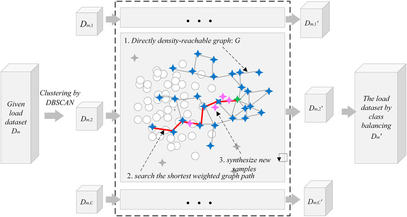
Motivated by the previous studies, this article initially presents a GSDC approach to solve the class imbalance issue. GSDC first constructs a directly density-reachable graph using density clustering. The algorithm then uses the shortest weighted graph path between the sample and the cluster centroid to form the sampling path to synthesize the minority samples. Then, the oversampling with the Gaussian stochastic perturbation is employed to enhance the diversities of the synthesized samples. This article will then present a fuzzy increment of diversity (FID) based clustering pruning strategy (CPS) to solve the base classifier redundancy issue. In this strategy, the FID eigenvector of each base classifier is firsts constructed. The FID characteristic matrix of all the base classifiers is then constructed. The affinity propagation clustering algorithm is then applied on the matrix to achieve the clusters and the corresponding centroids of the base classifiers. Based on two presented indices, the pruning strategy is implemented on the clusters. This finally leads us to achieve an optimal number of the base classifiers. To further maintain the diversity and accuracy of the redundancy eliminated base classifiers, a surrogate empirical risk with regular term-based optimization selection integration (OSI) composed of the surrogate empirical risk function, Huber function, and K-fold cross validation method is presented. Ultimately, combined with the popular classifiers, the performance of the presented class balancing algorithm and the improved selective ensemble learning algorithm are evaluated and validated.

The rest of this article is organized as follows. Section 2 presents the class balancing algorithm. Section 3 presents the improved selective ensemble learning algorithm. Section 4 shows the experimental results and discussions. Finally, Section 5 concludes this study.

2 Class balancing using GSDC

The class imbalance issue naturally exists in the load dataset, which increases the difficulties of minority class identification in the classifier. Although the stochastic oversampling algorithms can handle this issue to some extent, the flaws, for example, of the class overlapping and inaccurate sample distribution may deteriorate the performance of the classifier. Therefore, this article presents the GSDC algorithm to solve the flaws and improve the performance of the traditional SMOTE algorithm. It should be noted that there is currently no numerical definition of the concept minority class. Therefore, according to Liu et al. (2019), a threshold of 20% is employed to identify if a class is a minority class. If the number of the samples in a class is less than 20% of those in a class with the largest number of samples, then class is identified as a minority class.

2.1 Basic definitions in GSDC

1) $\rho$-neighborhood: Let $Z$ denote a cluster; $x_i$ denote a sample in $Z$; $x_j$ denote another sample in $Z$; and $\rho$ denote the neighborhood radius of $x_i$. Therefore, $\rho$-neighborhood $N_{\rho }\left(x_i\right)$ can be defined by Eq. 1:

$N_{\rho }\left(x_i\right)=\left\{x_j|\Vert x_i,x_j\Vert {\hspace{0.17em}}_2\le \rho ,x_j\in Z\right\}(1)$

2) Core: For a given sample $x_i$, if there are at least a number of $\kappa$ samples locating in its $\rho$ -neighborhood, then $x_i$ is regarded as a core.

3) Directly density-reachable: For two given samples $x_i$ and $x_j$, if $x_i$ is a core and $x_j$ satisfies $x_j\in N_{\rho }\left(x_i\right)$, then $x_j$ is regarded as directly density-reachable to $x_i$.

4) Directly density-reachable graph: Let $V$ denote the set of all the directly density-reachable samples in $Z$ and $E$ denote the set of edges, in each of which is a weighted graph path between a directly density-reachable sample and its core. The Euclidean distance between samples is employed as the weight. Therefore, $G(Z,\rho ,\kappa )=(V,E)$ is the direct density-reachable graph for the cluster $Z$ with parameters $\rho$ and $\kappa$.

2.2 Detailed steps of GSDC

Step 1, identify the minority sample and class. A given load dataset D is composed of samples belonged to a number of M classes $\left\{D_m|m=1,\cdots ,M\right\}$. If the number of samples in a class $D_m$ is smaller than 20% of the number of samples in the class which contains the largest number of samples, then $D_m$ is regarded as the minority class. The samples in $D_m$ are regarded as the minority samples.

Step 2, clustering of the minority samples. Let $D_m$ denote a minority set and $C$ denote the number of clusters in $D_m$. The DBSCAN clustering algorithm (Ester et al., 1996) is applied on $D_m$. Therefore, a number of clusters $\left\{D_{m,c}|c=1,\cdots ,C\right\}$ can be achieved. In addition, the centroids $\left\{x_c^{\text{center}}|c=1,\cdots ,C\right\}$ of the clusters can be achieved.

Step 3, direct density-reachable graph construction based on clusters. Based on the clustering results in Step 2, the directly density-reachable graph $G(D_{m,c},\rho ,\kappa )$ can be achieved according to Section 2.1. In this article, the values of $\rho$ and $\kappa$ are 10 and 3, respectively, according to the experiments based on the enumeration method.

Step 4, determine the number of synthesized samples for each $D_{m,c}$. Compute the proportion of the sample distribution for each cluster. Then, according to the proportion, the synthesized samples can be generated.

Step 5, search of the sampling path. In each sample synthetic operation, a real sample $x_r$ is randomly selected from $D_{m,c}$. The Dijkstra algorithm (Xu et al., 2007) is then employed to search the shortest weighted graph path $J_{r\leftrightarrow \text{center}}=x_r\leftrightarrow x_1^r\cdots x_{\alpha }^r\leftrightarrow x_{\beta }^r\cdots x_c^{\text{center}}$ between $x_r$ and the centroid $x_c^{\text{center}}$ in $G(D_{m,c},\rho ,\kappa )$. $x_1^r$, $x_{\alpha }^r$, and $x_{\beta }^r$ represent the samples that the path passes through. $\leftrightarrow$ represents directly density-reachable. As a result, $J_{r\leftrightarrow \text{center}}$ can be regarded as the sampling path.

Step 6, sample synthetic. A directly density-reachable edge $x_{\alpha }^r\leftrightarrow x_{\beta }^r$ is randomly selected from $J_{r\leftrightarrow center}$ as the sampling interval. In the sampling interval, an interpolation distance $\wp$ that is subject to the uniform distribution is employed, as shown in Eq. 2:

$\wp \sim U\left(0,d_{\alpha ,\beta }^r\right),d_{\alpha ,\beta }^r=\Vert x_{\alpha }^r-x_{\beta }^r\Vert {\hspace{0.17em}}_2(2)$

Then, randomly generate the interpolation coordinates $\vartheta$ shown in Eq. 3:

$\vartheta =\left(x_{\beta }^r-x_{\alpha }^r\right)\cdot \wp (3)$

Afterward, to improve the diversities of the synthesized samples, a random disturbance vector $o$ is added to $\vartheta$. $o$ subjects to the normal distribution, as shown in Eq. 4:

$o\sim N\left(0,d_{\alpha ,\beta }^r\cdot \sigma \right)(4)$

where $\sigma$ represents the relative standard deviation. Finally, one synthetic sample can be generated, which is presented by Eq. 5:

$x_{\text{synthetic}}=x_{\alpha }^r+\vartheta +o(5)$

Keep synthesizing the samples until the number of the samples in the minority class reaches to 20% of those in a class with the largest number of samples, the algorithm terminates.

The entire process of GSDC in enabling class balance of the load dataset is shown in Figure 1.

FIGURE 1

FIGURE 1. The entire process of GSDC in enabling class balance of the load dataset.

3 Improved selective ensemble learning

The essential method of the ensemble learning is based on one concept that a series of weak classifiers (base classifiers) are able to compose one strong classifier. The performance of the ensemble learning is depending on the diversity and the decision accuracy of the base classifier (Kuncheva and Whitaker, 2003; Yang et al., 2014). The diversity refers to the trend that the classifiers generate diverse misclassification of the samples, while the decision accuracy refers to the correct classification of the samples. It is obvious that along with the increasing scale of the base classifiers, the homogenization of the classifiers is inevitable. This point significantly deteriorates the diversity of the classifiers and finally causes the base classifier redundancy issue.

Therefore, to balance the diversity and accuracy of the classifiers, this article presents a fuzzy increment of diversity (FID) based clustering pruning strategy (CPS) and a surrogate empirical risk with regular term-based optimization selection integration (OSI) to implement the improved selective ensemble learning which finally serves the load classification and the identification of the load behaviors.

3.1 Clustering pruning strategy

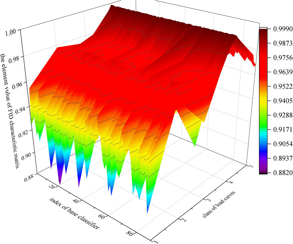
The presented fuzzy increment of diversity (FID) based clustering pruning strategy (CPS) first constructs the FID eigenvectors and the FID characteristic matrix for the base classifiers. The affinity propagation (AP) clustering algorithm is then applied on the matrix (Gan and Ng, 2014). According to the Euclidean distance-based and cosine distance-based measurement indices, the optimal centroids of the base classifiers can be achieved from the clustered clusters. This finally leads to the pruning of the redundancy base classifiers.

3.1.1 Eigenvector of FID

Q-statistics are employed to construct the FID eigenvector (Kuncheva and Whitaker, 2003). Q-statistics are able to measure the decision diversity between two base classifiers. The Q-statistic $Q_{u,v}^m$ of the base classifiers u and v for classifying the mth class of the load data can be represented by Eq. 6:

$Q_{u,v}^m=\frac{a_{u,v}{d}_{u,v}-b_{u,v}{c}_{u,v}}{a_{u,v}{d}_{u,v}+b_{u,v}{c}_{u,v}}(6)$

where $a_{u,v}$, $b_{u,v}$, $c_{u,v}$, and $d_{u,v}$ are subject to the joint distribution shown in Table 1.

TABLE 1

TABLE 1. Joint distribution for the two base classifiers.

In Table 1, $h_u\left(x_k\right)$ and $h_v\left(x_k\right)$ represent the classification results for the training sample $x_k$ using the base classifiers u and v, respectively; $y_k$ represents the class label of the training sample $x_k$; $a_{u,v}$ and $d_{u,v}$ represent the probabilities of <correct, correct> and <incorrect, incorrect> of classifying the training dataset using the base classifiers u and v respectively; and $b_{u,v}$ and $c_{u,v}$ represent the probabilities of <correct, incorrect> and <incorrect, correct> of classifying the training dataset using the base classifiers u and v, respectively. Therefore, according to Eqs. 5 and 6, the sum of pair-wise diversity index of a number of $L$ base classifiers can be represented by Eq. 7:

${\phi }_m={\displaystyle \sum _{u=1}^L{\displaystyle \sum _{v=u+1}^L{Q}_{u,v}^m}}(7)$

To delineate the impact of an individual base classifier on the sum of pair-wise diversity among all the base classifiers, the FID of the base classifier u in the mth class of the training dataset is defined using Eq.8:

${\mathrm{\Im }}_{u,m}={\phi }_m\left({\text{Ω}}_{u\not\subset \text{Ω}}\right)-{\phi }_m\left({\text{Ω}}_{u\subset \text{Ω}}\right)(8)$

where ${\text{Ω}}_{u\not\subset \text{Ω}}$ and ${\text{Ω}}_{u\subset \text{Ω}}$ represent the sets of all the base classifiers including and excluding the base classifier u. Therefore, the FID characteristic matrix for the base classifiers can be represented by Eq. 9:

$\Xi =\left[\begin{array}{ccccc}{\mathrm{\Im }}_{\mathrm{1,1}}& \dots & {\mathrm{\Im }}_{1,m}& \cdots & {\mathrm{\Im }}_{1,M}\\ ⋮& \ddots & ⋮& \ddots & ⋮\\ {\mathrm{\Im }}_{u,1}& \cdots & {\mathrm{\Im }}_{u,m}& \cdots & {\mathrm{\Im }}_{u,M}\\ ⋮& \ddots & ⋮& \ddots & ⋮\\ {\mathrm{\Im }}_{\text{L},1}& \cdots & {\mathrm{\Im }}_{\text{L},m}& \cdots & {\mathrm{\Im }}_{\text{L},M}\end{array}\right](9)$

3.1.2 Optimal number of centroids for base classifiers

The Euclidean distance and the cosine distance are frequently employed to measure the similarity between two data sequences. Based on the FID eigenvectors of all the base classifiers, the AP clustering algorithm is applied on the rows of $\Xi$ to generate a number of clusters. In each cluster, the mean Euclidean distance and the mean cosine distance between the centroid and certain FID eigenvector are then computed. This article presents the Euclidean redundancy index $\left(I_{\text{ERI}}\right)$ and the cosine redundancy index $\left(I_{\text{CRI}}\right)$ to facilitate the identification of the optimal centroid number. Two indices are represented by Eqs 10 and 11:

$I_{\text{ERI}}=\frac{2{\displaystyle {\sum }_{u=1}^{L_{\text{AP}}}{\displaystyle {\sum }_{v=u+1}^{L_{\text{AP}}}\Vert {\Xi }_{u,}-{\Xi }_{v,}{\Vert }_2}}}{L_{\text{AP}}\left(L_{\text{AP}}-1\right)}(10)$

$I_{\text{CRI}}=\frac{2{\displaystyle {\sum }_{u=1}^{L_{\text{AP}}}{\displaystyle {\sum }_{v=u+1}^{L_{\text{AP}}}{\Xi }_{u,}\cdot {\Xi }_{v,}}}}{L_{\text{AP}}\left(L_{\text{AP}}-1\right)\Vert {\Xi }_{u,}{\Vert }_2\cdot \Vert {\Xi }_{v,}{\Vert }_2}(11)$

where $L_{AP}$ represents the number of the centroids of the base classifiers. The larger $I_{\text{ERI}}$ or the smaller $I_{\text{CRI}}$ represents the greater diversity of the base classifiers in the cluster, and thus the redundancy of the base classifiers is regarded as lower. In the clustering processes, the optimal centroid number (the optimal number of the base classifier) can be achieved when the maximum and the minimum values of the indices are reached.

3.1.3 Steps of the presented CPS

Step 1: generate the base classifiers. In the load dataset $D$, based on the samples and their corresponding labels, a number of $L$ base classifiers can be generated using sampling and training. Any existing sampling algorithms and the supervised machine learning algorithms can be adopted to implement this step.

Step 2: Based on the generated base classifiers and the load dataset $D$, the Q-statistics of all the base classifier pairs are computed according to Eq. 6. Therefore, the FID eigenvectors of all the base classifiers can be achieved according to Eqs. 7 and 8. Finally, the characteristic matrix $\Xi$ can be formed using Eq. 9.

Step 3: Cluster the base classifiers. The AP clustering algorithm is applied once on the row vectors of the characteristic matrix $\Xi$. The number of the centroids can be achieved.

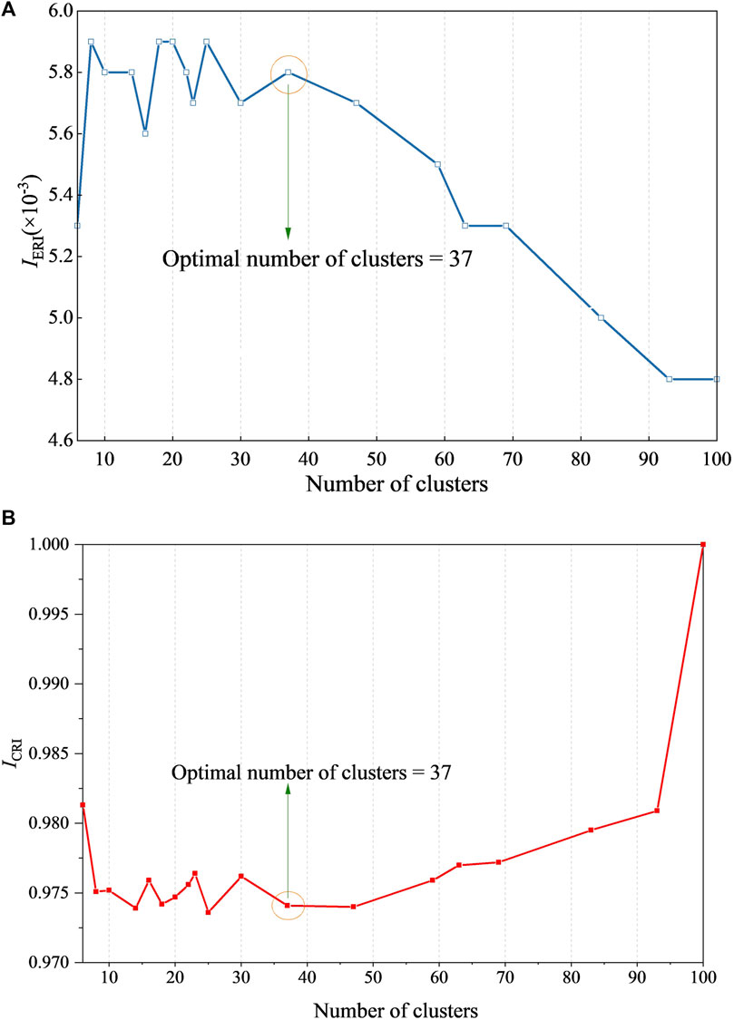
Step 4: Cluster pruning of the base classifiers. Keep executing Step 3 and compute $I_{\text{ERI}}$ and $I_{\text{CRI}}$ using Eqs 10 and 11, until the inflection points of the two indices appear. Therefore, the optimal number of centroids can be achieved. The base classifiers corresponding to the centroids are selected as the final classifiers. The base classifiers corresponding to the other points of the clusters are eliminated as redundancy.

3.2 Surrogate empirical risk with regular term-based optimization selection integration

To improve the generalization of the presented improved selective ensemble learning, this article further presents the OSI strategy. This strategy introduces the concept of ensemble margin to construct the minimum surrogate empirical risk with a regular term function to optimize the weights assigned to the base classifier in ensemble leaning.

3.2.1 Maximum ensemble margin strategy considering model complexity

Ensemble margin (Yang et al., 2014) is adopted to measure the correct classification tendency of the samples. Let $D_{\text{verify}}=\left\{(x_n,y_n)|n=1,\cdots ,N\right\}$ denote the verifying samples with labels; $N$ denote the number of the samples in $D_{\text{verify}}$; $(x_n,y_n)$ denote the nth sample and its corresponding label; ${\text{Ω}}_{\text{CPS}}$ denote the set of the pruned base classifiers; and $H\left(X\right)=\left\{h_u\left(x_n\right)|x_n\subset D_{\text{verify}};u\subset {\text{Ω}}_{\text{CPS}}\right\}$ denote the classification results of using the base classifiers in ${\Omega }_{CPS}$ to classify the $D_{\text{verify}}$. Therefore, the ensemble margin $\Upsilon (x_n,y_n)$ of ${\text{Ω}}_{\text{CPS}}$ to sample $x_n$ can be represented by Eq. 12:

$\gamma \left(x_n,y_n\right)=y_n\cdot \varsigma \left(x_n\right)=y_n{\displaystyle \sum _{u=1}^{L_{\text{AP}}}{\upsilon }_u}{h}_u\left(x_n\right)\left({\displaystyle \sum _{u=1}^{L_{\text{AP}}}{\upsilon }_u}=\mathrm{1,0}\le {\upsilon }_u<1\right)(12)$

where ${\upsilon }_u$ denotes the weight of base classifier u in the ensemble learning and $\varsigma \left(x_n\right)$ denotes the classification result using the base classifiers-based ensemble learning. If the classification result is correct, then $y_n\varsigma \left(x_n\right)=1$, and otherwise $y_n\varsigma \left(x_n\right)=-1$. Based on the ensemble margin, the empirical risk function can be represented by Eq. 13:

${\ell }_{\text{loss}}\left(H\left(X\right)\right)={\displaystyle \sum _{n=1}^N\left(1-{\displaystyle \sum _{u=1}^{L_{\text{AP}}}{\upsilon }_u}{y}_n{h}_u\left(x_n\right)\right)}={\displaystyle \sum _{n=1}^N\left(1-\gamma \left(x_n,y_n\right)\right)}(13)$

The presented OSI is able to improve the generalization of the classification model using the loss function. Furthermore, to control the complexity of the ensemble learning and reduce the overfitting caused by the optimization, this article also presents Eq. 14 considering the regular term in the weights of the base classifiers, which is an optimization problem:

$\begin{array}{l}\underset{\mathit{\upsilon }}{\text{min}}{\mathit{\Vert v\Vert }}_2^2+\mu {\ell }_{\text{loss}}\left(H\left(X\right)\right)\hfill \\ \begin{array}{cc}s.t.& {\displaystyle \sum _{u=1}^{L_{\text{AP}}}{\upsilon }_u}=1\left({\upsilon }_u\ge 0\right)\end{array} \hfill \end{array}(14)$

where $\mathit{\upsilon }=({\upsilon }_1\cdots {\upsilon }_u\cdots {\upsilon }_{L_{\text{AP}}})$; regular term ${\mathit{\upsilon }}_2^2$ controls the complexity of the ensemble learning model; and $\mu >0$ is the equivalence factor.

3.2.2 Huber function based surrogate empirical risk function

The loss function ${\ell }_{\text{loss}}\left(H\left(X\right)\right)$ in Eq. 14 is nonconvex and discontinuous, which results in difficulties of optimization. However, surrogate empirical risk function has been reported as a proper way of solving this issue. In this article, the truncated Huber function (Borah and Gupta, 2020) shown in Eq. 15 is employed as the surrogate empirical risk function. A factor $\mathrm{\epsilon }$ is also adopted to tune the sensitivity of the surrogate empirical risk function to the outliers and noises. In the following experiments, the value of $\mathrm{\epsilon }$ is set to 0.6.

$f_{\text{Huber}}\left[w\right]=\{\begin{array}{c}\mathrm{\epsilon }\cdot w-{\mathrm{\epsilon }}^2/2\\ w^2/2\\ 0\end{array}\begin{array}{cc},& \begin{array}{c}0<w\le 1-\mathrm{\epsilon }\\ 1-\mathrm{\epsilon }<w\le 1\\ w>1\end{array}\end{array}(15)$

Finally, based on Eqs. 15 and 14 can be reformed into Eq. 16, which is ultimately employed to optimize the participating weights of the base classifiers:

$\begin{array}{c}\underset{\mathit{\upsilon }}{\text{min}}{\mathit{\Vert v\Vert }}_2^2+\mu {\displaystyle \sum _{n=1}^N{f}_{\text{Huber}}}\left[1-\gamma \left(x_n,y_n\right)\right]\\ \begin{array}{cc}s.t.& {\displaystyle \sum _{u=1}^{L_{\text{AP}}}{\upsilon }_u}=1\left({\upsilon }_u\ge 0\right)\end{array}\end{array}(16)$

3.2.3 K-fold cross validation method-based base classifier selection

K-fold cross validation method is adopted to achieve a number of K verifying datasets $D_{\text{verify}}$ from the original labeled training dataset. Repeat the presented OSI strategy in each $D_{\text{verify}}$ to finally generate a number of K-time optimized weights for ${\text{Ω}}_{\text{CPS}}$, which is shown by Eq. 17:

$\Lambda =\left[\begin{array}{ccccc}{\upsilon }_{\mathrm{1,1}}& \cdots & {\upsilon }_{1,u}& \cdots & {\upsilon }_{1,L_{\text{AP}}}\\ ⋮& \ddots & ⋮& \ddots & ⋮\\ {\upsilon }_{s,1}& \cdots & {\upsilon }_{s,u}& \cdots & {\upsilon }_{s,L_{\text{AP}}}\\ ⋮& \ddots & ⋮& \ddots & ⋮\\ {\upsilon }_{\text{Κ},1}& \cdots & {\upsilon }_{\text{Κ},u}& \cdots & {\upsilon }_{K,L_{\text{AP}}}\end{array}\right](17)$

where ${\upsilon }_{s,u}$ denotes the optimized weight of the uth base classifier in the sth time OSI execution. Let $\left[{\upsilon }_{1,u},\cdots ,{\upsilon }_{s,u},\cdots ,{\upsilon }_{\text{K},u}\right]$ denote a number of K-time optimized weights of the base classifier u in ${\text{Ω}}_{\text{CPS}}$. Calculate the proportion of the times in which the weight is greater than 0 according to Eq. 18:

${\mathrm{\Re }}_u=\frac{{{\displaystyle \sum }}_{s=1}^{\text{K}}\text{max}\left(0,\text{sign}\left({\upsilon }_{s,u}\right)\right)}{\text{K}}(18)$

where the value of the function $\text{sign}(\cdot )$ is 1 when ${\upsilon }_{s,u}$ is greater than 0, otherwise the value of the function $\text{sign}(\cdot )$ is −1. When ${\mathrm{\Re }}_u\ge 0.5$, the corresponding base classifier is retained and will participate in the final majority voting-based ensemble learning for load classification.

3.3 Steps of the presented improved selective ensemble learning approach in enabling load classification

Step 1: A dataset $D$ consisting of the labeled samples is initially divided into a number of M sub-classes according to the labels $\left\{D_m|m=1,\cdots ,M\right\}$. In each sub-class, the samples are randomly divided into the training dataset $D_{\text{train},m}$ and the testing dataset $D_{\text{test},m}$ with the ratio 4:6. In $D_{\text{train},m}$, the minority classes are processed by GSDC to balance the data distribution. Finally, merge all of the sub-training datasets and the testing datasets to achieve $D_{\text{train}}^{\nearrow }$ and $D_{\text{test}}$.

Step 2: In $D_{\text{train}}^{\nearrow }$, bootstrap sampling is carried out to generate a number of $L$ sub-datasets. The samples in the sub-datasets and their labels are input into a number of $L$ initiated classifiers. The Adam algorithm is further employed to optimize the loss function for each classifier. The early stop strategy is adopted to determine the number of the iterations of the classifier learning. Finally, a number of $L$ trained base classifiers can be achieved, and the set of the base classifier $\text{Ω}$ can be formed.

Step 3: Each base classifier in $\text{Ω}$ classifies $D_{\text{train}}^{\nearrow }$, therefore the classification result $H_{\text{train}}\left(X\right)=\left\{h_u\left(x_k\right)|x_k\subset D_{\text{train}}^{\nearrow };u\subset \text{Ω}\right\}$ can be achieved. Based on $H_{\text{train}}\left(X\right)$, the FID characteristic matrix $\Xi$ can be constructed according to Eqs. 6–9.

Step 4: The presented CPS is then applied on $\Xi$. The AP clustering algorithm clusters the FID eigenvectors in $\Xi$ of all the base classifiers. According to Eqs. 10 and 11, the optimal number of the centroids $L_{\text{AP}}$ can be achieved based on the pruning of CPS. The corresponding retained base classifiers form a set ${\text{Ω}}_{\text{CPS}}$.

Step 5: In the presented OSI phase, K-fold cross validation method is adopted. $D_{\text{train}}^{\nearrow }$ is randomly divided into a number of K equal parts according to the proportion of the classes, each part is represented by $\left\{D_{\text{verify},s}\subseteq D_{\text{train}}^{\nearrow }|s=1,\cdots ,K\right\}$.

Step 6: Each base classifier in ${\text{Ω}}_{\text{CPS}}$ classifies $D_{\text{verify},s}$. The classification result is represented by $H_{\text{test}}\left(X\right)=\left\{h_u\left(x_k\right)|x_k\subset D_{\text{verify},s};u\subset {\text{Ω}}_{\text{CPS}}\right\}$. According to Eqs. 12–16, the weights of the base classifiers in ${\text{Ω}}_{\text{CPS}}$ can then be computed.

Step 7: Repeat Step 6 for K times. According to Eq. 17, the K-time weights $\Lambda$ of the base classifier can then be achieved.

Step 8: For each base classifier in ${\text{Ω}}_{\text{CPS}}$ (e.g., the base classifier $u$), according to Eq. 18 compute ${\mathrm{\Re }}_u$. If the value of ${\mathrm{\Re }}_u$ is greater than 0.5, then the corresponding base classifier $u$ is retained and will participate the final majority voting-based ensemble learning for classifying $D_{\text{test}}$.

4 Experimental results

4.1 The datasets employed to evaluate the presented approach

This article mainly employs three load datasets including the synthetic binary dataset, Electrical Grid Stability Simulated Dataset (EGSSD) (Arzamasov, 2018), and Electricity Load Diagrams 20112014 Dataset (ELDD) (Trindade, 2015). The samples in the synthetic binary dataset are labeled. The samples in EGSSD are also already labeled (system stability and system instability). In contrast, the samples in ELDD are not labeled. Therefore, the labels of the samples in ELDD can be achieved using the approach presented by Liu et al. (2019). The details of three datasets are listed in Table 2.

TABLE 2

TABLE 2. Detailed information of the synthetic binary, EGSSD, and ELDD datasets.

The sampling interval for each sample in ELDD is 15 min. Therefore, in 1 day there are 96 sampling points in total. According to the sample dimension 140,256, each sample contains the load information for 1,461 days. In terms of analyzing the load data for 1 day, each sample in ELDD is converted into the daily load. As a result, the finally converted ELDD dataset contains $370\times (140256/96)=370\times 1461=540570$ samples, each of which has 96 dimensions.

4.2 Indices employed to evaluate the classification performance

Besides the accuracy A_cc, which represents the overall classification accuracy of the samples is employed to evaluate the performance of the binary classification, the recall P_re and the precisions including P_pr, G_means, and F_value are also employed (López et al., 2013). P_re represents the proportion of the correctly classified minority samples. P_pr represents the real proportion of the minority samples in the samples that are classified as the minority samples. G_means represents the geometric mean of the proportion of the correctly classified samples in all majority classes and the proportion of the correctly classified samples in all minority classes. G_means presents the tendency of the classifiers of classifying different classes. If the value of G_means is close to the value of A_cc, then the performance of the presented class balancing approach can be regarded as better. F_value represents the harmonic mean of P_re and P_pr. A greater value of F_value indicates that the improvements of classifying the minority classes generate less impact on classifying the majority classes.

Although the confusion matrix is frequently employed in multi-class classification evaluations, it is difficult to quantitatively assess the performance of the classification model. Therefore, based on the confusion matrix, this article presents the index named as the class confusion equilibrium entropy. The equations composing the index are presented as follows. First, the confusion matrix of binary classification $M_{\text{confusion}}$ can be denoted by Eq. 19:

$M_{\text{confusion}}=\left[\begin{array}{cc}{N}_{\text{TP}}& N_{\text{FP}}\\ N_{\text{FN}}& N_{\text{TN}}\end{array}\right](19)$

where $N_{\text{TP}}$ and $N_{\text{TN}}$ represent the number of samples correctly classified as positive and negative classes, respectively; and $N_{\text{FP}}$ and $N_{\text{FN}}$ represent the number of samples misclassified as positive class and the number of samples misclassified as negative class, respectively. In multi-class classification, the confusion matrix can be regarded as a combination of multiple binary confusion matrices. In the confusion matrix, the target class is treated as the positive class and the other classes are treated as the negative classes. We then define the harmonic average accuracy of the binary classification when the mth class is classified as the positive class using Eq. 20:

${\Gamma }_m=\frac{2N_{\text{TP}}{N}_{\text{TN}}}{N_{\text{TP}}\left(N_{\text{TN}}+N_{\text{FP}}\right)+N_{\text{TN}}\left(N_{\text{TP}}+N_{\text{FN}}\right)}(20)$

${\Gamma }_m$ is able to measure the class confuse level of the binary classification scenario. A smaller value of ${\Gamma }_m$indicates a more severe confusion level. Based on Eq. 20, the class confusion equilibrium entropy is presented by Eq. 21:

$S_{\text{b}}=-{\displaystyle \sum }_{m=1}^M\frac{{\Gamma }_m}{{{\displaystyle \sum }}_{m=1}^M{\Gamma }_m}\ln \frac{{\Gamma }_m}{{{\displaystyle \sum }}_{m=1}^M{\Gamma }_m}(21)$

A greater value of S_b represents more equilibrium of the class confusion for the classifier, which also indicates the better class balancing performance of the presented GSDC algorithm.

4.3 Evaluation of GSDC

To evaluate the performance of the presented GSDC algorithm, this section employs the synthetic binary dataset, EGSSD dataset, and ELDD dataset. As aforementioned, the EGSSD dataset contains two classes and the ELDD dataset contains multiple classes.

4.3.1 Experiments using the synthetic binary dataset

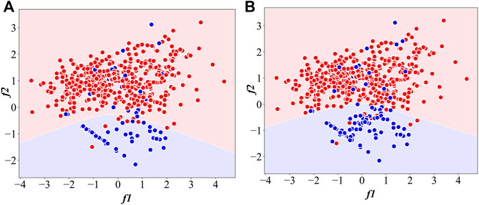
The classification experiment is carried out using the synthetic binary dataset. The ratio of the minority class (in blue) and the majority class (in red) is 1:10. Support vector machine (SVM) is employed as the classifier.

Figure 2B shows that, based on the class balance using the presented GSDC algorithm, the sample distribution can be positively enhanced. The samples of the minority class can be significantly highlighted. Compared to the classification result without being processed by GSDC, as shown in Figure 2A, the hyperplane of SVM in Figure 2B is improved. Additionally, the minority samples in the area overlapping with the majority samples are not obviously affected by GSDC. Therefore, the presented class balancing strategy only has a limited influence on the classification of the majority samples, which demonstrates that GSDC can effectively synthesize the minority samples according to the sample distribution characteristic.

FIGURE 2

FIGURE 2. The classification (A) without processing by GSDC and (B) with processing by GSDC.

4.3.2 Experiments using the EGSSD dataset

First, the testing dataset is generated. In total, 2000 samples are randomly selected form the transient stability class and the transient instability class to form the testing dataset. Second, the training dataset is generated. A number of 4,000 transient stability samples and a number of 400 transient instability samples are also randomly selected to form the training dataset. The back propagation neural network (BPNN) classifier is employed in this section. In addition, the conventional SMOTE and BS class balancing algorithms are also implemented in terms of comparison. The classification results are listed in Table 3.

TABLE 3

TABLE 3. Classification results based on the EGSSD dataset with different class balancing algorithms.

According to the results shown in Table 3, if the classification is carried out without class balancing, then due to the insufficient training of the minority class, the samples belonged to the minority class have higher chances to be misclassified. This results in higher $P_{pr}$ but lower $P_{\text{re}}$. In addition, the overall classification accuracy A_cc is low. Based on the class balancing algorithms including SMOTE, BS, and GSDC, the classification accuracy A_cc is significantly improved. In particular, the classification accuracy and the other indices based on GSDC outperform those of the other class balancing algorithms. The error between $G_{\text{means}}$ and A_cc is only 0.0007, which means that GSDC can supply satisfactory class balancing performance. The highest value of $F_{value}$ indicates that GSDC has the smallest impact on the classification for the majority class. The evaluation suggests that GSDC has better global performances.

To evaluate the impact of the imbalance class proportion on the performance of GSDC, a series of the training datasets are generated. First, 4,000 samples belonged to the transient instability class are randomly selected. Then, based on the ratios of 20:1, 40:1, 80:1, and 160:1, the corresponding numbers of the samples belonged to the transient stability class are randomly selected. Therefore, four imbalanced training datasets can be achieved. The classification results are listed in Table 4.

TABLE 4

TABLE 4. lassification accuracy based on different imbalance ratios.

It can be observed that along with the increasing imbalance ratio, the classification accuracies based on different class balancing algorithms gradually deteriorate. This means that in the extremely imbalanced dataset, the balancing algorithm can supply limited improvement in terms of the classification accuracy. However, GSDC still outperforms the other algorithms.

4.3.3 Experiments using the ELDD dataset

The samples in ELDD are not labeled, which causes difficulty in their classification. Therefore, according to Liu et al. (2019), the labeling operation is applied on the dataset, and therefore the labeled dataset can be achieved. In terms of facilitating the experiments, a labeled subset $D$ that contains five classes and 16,620 samples is generated from the original ELDD. Then, $D$ is divided into the training dataset $D_{\text{train}}$ and the testing dataset $D_{\text{test}}$ in the ratio of 4:6. In the training dataset, the numbers of samples belonged to the five classes are 3,770, 1,502, 284, 320, and 818, respectively, of which the samples belonged to the third and the fourth classes are regarded as the minority samples. Afterward, based on GSDC, the imbalanced classes in $D_{\text{train}}$ are balanced to generate the balanced training dataset $D_{\text{train}}^{\nearrow }$. BPNN is also employed as the classifier. The classification results based on different class balancing algorithms and different levels of noise are listed in Figures 3, 4. Additionally, white noise is employed in the following experiments. Noise level refers to the amplitude of the noise. Each noise sample is added to a training sample in $D_{\text{train}}$. Therefore, the borders of the training samples are blurred, which is suitable to evaluate the class balancing ability of GSDC.

FIGURE 3

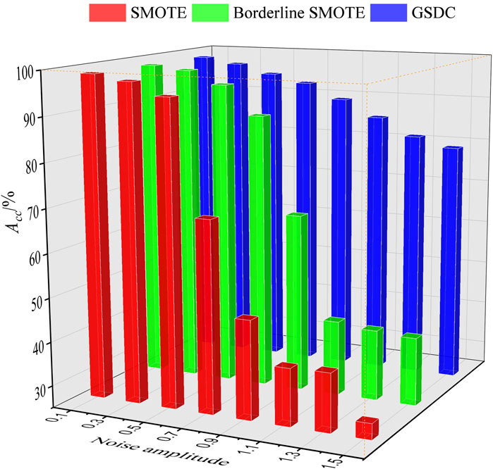
FIGURE 3. The classification accuracy based on different class balancing algorithms and different levels of noise.

FIGURE 4

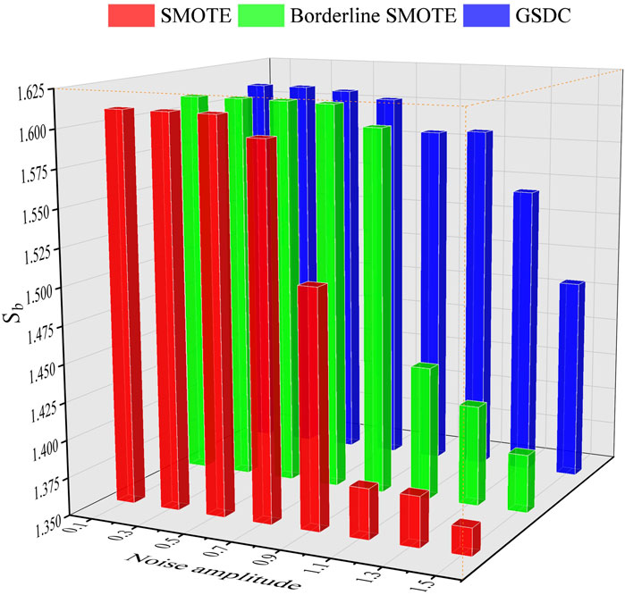
FIGURE 4. The values of S_b based on different class balancing algorithms and different levels of noise.

From Figures 3, 4, it can be observed that when the noise level is low, with the improvements of the class balancing algorithms, the accuracy of the classification results is quite similar. However, along with the increasing noise level, especially when the level reaches 0.9, the accuracy A_cc and values of S_b of the classification based on SMOTE and BS sharply decreased. In contrast, the accuracy A_cc and values of S_b of the classification based on the presented GSDC still maintain higher levels. This point significantly suggests that GSDC has great abilities in terms of robust and noise immunity.

4.4 Evaluation of the improved selective ensemble learning approach

4.4.1 The parameters employed in the evaluation

The base classifiers employed in the evaluation include BPNN, classification and regression tree (CART), and long short-term memory neural network (LSTM). The performance of the presented improved selective ensemble learning approach is based on the classification performance of these base classifiers. First, according to step 2 in Section 3.3, a total of 100 labeled training sub-datasets are generated based on $D_{\text{train}}^{\nearrow }$ using bootstrapping (the bootstrapped number of samples equals to the sample number of the original dataset). Then, 100 BPNN base classifiers are trained using the training sub-datasets. Therefore, the FID characteristic matrix $\Xi$ of these base classifiers can be achieved. The elements of the matrix $\Xi$ are shown in Figure 5.

FIGURE 5

FIGURE 5. The FID characteristic matrix of 100 BPNN base classifiers.

According to step 4 in Section 3.3, the CPS strategy is then applied on the base classifiers. The redundancy removed set of base classifiers can be achieved.

Figures 6A,B indicate that when $L_{\text{AP}}$ reaches 37, the indices $I_{\text{ERI}}$ and $I_{\text{CRI}}$ become roughly stable and monotonic. In this case, the centroids of the clusters are kept, as well as the corresponding base classifiers to form the redundancy removed set of the base classifiers ${\text{Ω}}_{\text{CPS}}$. Afterward, OSI is applied further. To determine a proper value of $\mu$ in Eq. 14, this article exponentially increases the value of $\mu$ from 0.001 to 100. When the value of equivalence factor $\mu$ reaches 1, the weights of base classifiers become stable. Therefore, in the OSI phase, the value of $\mu$ is determined as 1.

FIGURE 6

FIGURE 6. The value variations of (A) I_ERI and (B) I_CRI.

4.4.2 Performance evaluation of load classification using ELDD

According to steps 5 to 7 in Section 3.3, A five-fold cross validation is employed in this section. Repeat step 5 for five times, in each of which the weights of base classifiers in ${\text{Ω}}_{\text{CPS}}$ can be computed. The weight matrix $\Lambda$ can then be formed. According to step 8 in Section 3.3, the OSI phase finally retains nine base classifiers, which can be ultimately employed to classify $D_{\text{test}}$ based on the majority voting.

BPNN, CART, and LSTM algorithms are adopted as the base classifiers, on which the improved selective ensemble learning is applied. In terms of comparison, famous ensemble learning strategies, including bagging and adaboosting, are also implemented. Based on the presented approach, and other ensemble learning strategies, the classification results including A_cc and S_b of classifying $D_{\text{test}}$ are listed in Tables 5, 6.

TABLE 5

TABLE 5. omparisons of the accuracy of different ensemble learning strategies.

TABLE 6

TABLE 6. omparisons of S_b of different ensemble learning strategies.

From Tables 5, 6, it can be observed that in terms of A_cc and S_b, the presented approach outperforms the famous ensemble learning algorithms including bagging and adaboosting. In addition, the classification results suggest that the presented approach is able to serve different classifiers with significant performance improvement.

4.4.3 Stability evaluations of the improved selective ensemble learning

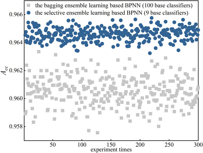
To demonstrate the stability of the presented improved selective ensemble learning based load classification, this section employs BPNN as the base classifier. GSDC is employed to balance the testing dataset $D_{\text{train}}^{\nearrow }$ of ELDD. Bagging is also implemented in terms of comparison. Both the classifications for the testing dataset $D_{\text{test}}$ using the presented improved selective ensemble learning based BPNN (9 base classifiers) and the bagging ensemble learning based BPNN (100 base classifiers) are carried out 300 times. The results are shown in Figure 7.

FIGURE 7

FIGURE 7. A comparison of the stability of two ensemble learning approaches.

Figure 7 first shows that in 300-time experiments, although more base classifiers involved in bagging, the improved selective ensemble learning based BPNN outperforms the bagging ensemble learning based BPNN in terms of classification accuracy. Second, the improved selective ensemble learning also performs a correspondingly stable performance. The accuracies of 300-time experiments are quite close. The results shown in Figure 7 prove that the presented selective ensemble learning can improve both the classification accuracy and the classification stability.

5 Conclusion

Class imbalance and low efficiency prevent load classification from being effectively carried out. Therefore, this article presents an improved selective ensemble learning approach to enable load classification considering base classifier redundancy and class imbalance. First, a Gaussian SMOTE based on density clustering is proposed. The minority samples can be effectively synthesized, mainly using sampling techniques, DBSCAN clustering algorithm, and Dijkstra algorithm. Therefore, the original dataset can be significantly balanced. Second, a fuzzy increment of diversity based clustering pruning strategy is further proposed. Based on FID characteristic matrix and AP clustering algorithm, the redundancy of the base classifiers can be discovered and removed. To improve the generalization of the classification model, the ensemble margin based empirical risk function, the Huber loss function, and the K-fold cross validation method-based optimization selection integration are proposed. According to the experimental results, the presented GSDC is able to effectively balance the classes, which finally leads to an improvement of the classification accuracy. The presented CPS and OSI strategies can also remove the redundancy of the base classifiers, which significantly improves the efficiency of the ensemble learning. All of the positive results indicate that the presented improved selective ensemble learning approach considering base classifier redundancy and class imbalance can be an effective tool to serve practical large-scale load classification tasks.

Data availability statement

The original contributions presented in the study are included in the article/Supplementary Material, and further inquiries can be directed to the corresponding author.

Author contributions

The authors contributed their original works respectively for this article. SW and YL presented the basic idea of the article. They also presented the employed algorithms of the article. DH, YH, and LW implemented the algorithms and further presented the experiments of evaluating and validating the performances of the algorithms. YW organized and structures the article and finally finished the writing works.

Funding

The authors would like to appreciate the support from the State Grid Henan Economic Research Institute with the project “Big Data based Residential Load Data Identification, Analysis, and Power Consumption Management Research” under Grant No. 5217L021000C.

Conflict of interest

SW, DH, YH, and YW are employed by State Grid Henan Electric Power Company.

The remaining authors declare that the research was conducted in the absence of any commercial or financial relationships that could be construed as a potential conflict of interest.

Publisher’s note

All claims expressed in this article are solely those of the authors and do not necessarily represent those of their affiliated organizations, or those of the publisher, the editors, and the reviewers. Any product that may be evaluated in this article, or claim that may be made by its manufacturer, is not guaranteed or endorsed by the publisher.

References

Aderibole, A., Zeineldin, H. H., Hosani, M. A., and El-Saadany, E. F. (2019). Demand side management strategy for droop-based autonomous microgrids through voltage reduction. IEEE Trans. Energy Convers. 34 (2), 878–888. doi:10.1109/TEC.2018.2877750

CrossRef Full Text | Google Scholar

Arzamasov, V. (2018). Data from: Electrical Grid stability simulated data dataset. Orange County, California: Machine Learning Repository. Available at: http://archive.ics.uci.edu/ml/machine-learning-databases/00471/.

Google Scholar

Borah, P., and Gupta, D. (2020). Functional iterative approaches for solving support vector classification problems based on generalized Huber loss. Neural comput. Appl. 32 (13), 9245–9265. doi:10.1007/s00521-019-04436-x

CrossRef Full Text | Google Scholar

Ester, M., Kriegel, H-P., Sander, J., and Xu, X. (1996). “A density-based algorithm for discovering clusters in large spatial databases with noise,” in The 2nd international conference on knowledge discovery and data mining (Portland, Oregon, USA: AAAI), 226–231.

Google Scholar

Gan, G., and Ng, M. K. -P. (2014). Subspace clustering using affinity propagation. Pattern Recognit. DAGM. 48, 1455–1464. doi:10.1016/j.patcog.2014.11.003

CrossRef Full Text | Google Scholar

Kuncheva, L. I., and Whitaker, C. J. (2003). Measures of diversity in classifier ensembles and their relationship with the ensemble accuracy. Mach. Learn. 51 (2), 181–207. doi:10.1023/A:1022859003006

CrossRef Full Text | Google Scholar

Li, X., Wang, P., Liu, Y., and Xu, L. (2020). Massive load pattern identification method considering class imbalance. Proc. CSEE 40 (01), 128–137+380. doi:10.13334/j.0258-8013.pcsee.190098

CrossRef Full Text | Google Scholar

Liu, S., Reviriego, P., HernÁndez, J. A., and Lombardi, F. (2021). Voting margin: A scheme for error-tolerant k nearest neighbors classifiers for machine learning. IEEE Trans. Emerg. Top. Comput. 9 (4), 2089–2098. doi:10.1109/TETC.2019.2963268

CrossRef Full Text | Google Scholar

Liu, W. (2021). “Cooling, heating and electric load forecasting for integrated energy systems based on CNN-LSTM,” in 2021 6th international conference on power and renewable energy (ICPRE) (Shanghai, China: IEEE). doi:10.1109/ICPRE52634.2021.9635244

CrossRef Full Text | Google Scholar

Liu, Y., Gao, L., and Liu, L. (2020a). Parallel load type identification algorithm considering sample class imbalance. Power Syst. Technol. 44 (11), 4310–4317. doi:10.13335/j.1000-3673.pst.2020.0116

CrossRef Full Text | Google Scholar

Liu, Y., Li, X., and Chen, X. (2020b). High-performance machine learning for large-scale data classification considering class imbalance. Scientific Programming. doi:10.1155/2020/1953461

CrossRef Full Text | Google Scholar

Liu, Y., Liu, Y., Xu, L., and Wang, J. (2019). A high performance extraction method for massive user load typical characteristics considering data class imbalance. Proc. CSEE 39 (14), 4093–4104. doi:10.13334/j.0258-8013.pcsee.181495

CrossRef Full Text | Google Scholar

Liu, Y., Ma, C., Xu, L., Shen, X., Li, M., and Li, P. (2017). MapReduce-based parallel GEP algorithm for efficient function mining in big data applications. Concurr. Comput. Pract. Exper. 30, e4379. doi:10.1002/cpe.4379

CrossRef Full Text | Google Scholar

Liu, Y., Xu, L., and Li, M. (2016). The parallelization of back propagation neural network in MapReduce and spark. Int. J. Parallel Program. 45, 760–779. doi:10.1007/s10766-016-0401-1

CrossRef Full Text | Google Scholar

López, V., Fernandez, A., Garcia, S., Palade, V., and Herrera, F. (2013). An insight into classification with imbalanced data: Empirical results and current trends on using data intrinsic characteristics. Inf. Sci. 250, 113–141. doi:10.1016/j.ins.2013.07.007

CrossRef Full Text | Google Scholar

Muthirayan, D., Kalathil, D., Poolla, K., and Varaiya, P. (2000). Mechanism design for demand response programs. IEEE Trans. Smart Grid 11 (1), 61–73. doi:10.1109/TSG.2019.2917396

CrossRef Full Text | Google Scholar

Shi, L., Zhou, R., and Zhang, W. (2019). Load classification method using deep learning and multi-dimensional fuzzy C-means clustering. Proc. CSU-EPSA 31 (7), 43–50. doi:10.19635/j.cnki.csu-epsa.000089

CrossRef Full Text | Google Scholar

Tambunan, H. B., Barus, D. H., Hartono, J., Alam, A. S., Nugraha, D. A., and Usman, H. H. H. (2020). “Electrical peak load clustering analysis using K-means algorithm and silhouette coefficient,” in 2020 international conference on technology and policy in energy and electric power (ICT-PEP) (Bandung, Indonesia: IEEE). doi:10.1109/ICT-PEP50916.2020.9249773

CrossRef Full Text | Google Scholar

Tang, Z., Liu, Y., and Xu, L. (2020). Imbalanced-load pattern extraction method based on frequency domain characteristics of load data and LSTM network. Electr. Power Constr. 41 (8), 17–24. doi:10.12204/j.issn.1000-7229.2020.08.003

CrossRef Full Text | Google Scholar

Trindade, A. (2015). Data from: ElectricityLoadDiagrams20112014 dataset. Orange County, California: Machine Learning Repository. Available at: http://archive.ics.uci.edu/ml/machine-learning-databases/00321/.

Google Scholar

Wang, L., Liu, Y., Li, W., Zhang, J., Xu, L., and Xing, Z. (2022). Two-stage power user classification method based on digital feature portraits of power consumption behavior. Electr. Power Constr. 43 (2), 70–80. doi:10.12204/j.issn.1000-7229.2022.02.009

CrossRef Full Text | Google Scholar

Wang, Z., Li, H., Tang, Z., and Liu, Y. (2021). User-level ultra-short-term load forecasting model based on optimal feature selection and bahdanau attention mechanism. J. Circuits, Syst. Comput. 30. doi:10.1142/S0218126621502790

CrossRef Full Text | Google Scholar

Wei, Z., Ma, X., and Guo, Y. (2022). Optimized operation of integrated energy system considering demand response under carbon trading mechanism. Electr. Power Constr. 43 (1), 1–9. doi:10.12204/j.issn.1000-7229.2022.01.001

CrossRef Full Text | Google Scholar

Xu, M. H., Liu, Y. Q., Huang, Q. L., Zhang, Y., and Luan, G. (2007). An improved dijkstra's shortest path algorithm for sparse network. Appl. Math. Comput. 185 (1), 247–254. doi:10.1016/j.amc.2006.06.094

CrossRef Full Text | Google Scholar

Yang, C., Yin, X. C., and Hao, H. W. (2014). Classifier ensemble with diversity: Effectiveness analysis and ensemble optimization. Acta Autom. Sin. 40 (4), 660–674. doi:10.3724/SP.J.1004.2014.00660

CrossRef Full Text | Google Scholar

Zhang, J., Liu, Y., Li, W., Wang, L., and Xu, L. (2022). Power load curve identification method based on two-phase data enhancement and Bi-directional deep residual TCN. Electr. Power Constr. 43 (2), 89–97. doi:10.12204/j.issn.1000-7229.2022.02.011

CrossRef Full Text | Google Scholar

Zhang, M., Li, L., and Yang, X. (2020). A load classification method based on Gaussian mixture model clustering and multi-dimensional scaling analysis. Power Syst. Technol. 44 (11), 4283–4296. doi:10.13335/j.1000-3673.pst.2019.1929

CrossRef Full Text | Google Scholar

Zhang, P., Wu, X., Wang, X., and Bi, S. (2015). Short-term load forecasting based on big data technologies. CSEE Power Energy Syst. 1 (3), 59–67. doi:10.17775/CSEEJPES.2015.00036

CrossRef Full Text | Google Scholar

Zhou, K., and Yang, S. (2012). An improved fuzzy C-Means algorithm for power load characteristics classification. Power Syst. Prot. Control 40 (22), 58–63. CNKI:SUN:JDQW.0.2012-22-013.

Google Scholar

Zhu, Q., Zheng, H., and Tang, Z. (2021). Load scenario generation of integrated energy system using generative adversarial networks. Electr. Power Constr. 42 (12), 1–8. doi:10.12204/j.issn.1000-7229.2021.12.001

CrossRef Full Text | Google Scholar

Zhu, T., Ai, Q., and He, X. (2020). An overview of data-driven electricity consumption behavior analysis method and application. Power Syst. Technol. 44 (9), 3497–3507. doi:10.13335/j.1000-3673.pst.2020.0226a

CrossRef Full Text | Google Scholar