Model predictive power control of a heat pipe cooled reactor

Heat pipe cooled reactor (HPR) has broad application prospects in deep space exploration, deep-sea submarine exploration, and other scenarios due to the small size, high inherent safety, and easy modularization and expansion. However, the HPR conducts thermal energy through evaporation and condensation of the working fluid inside the heat pipe. This feature makes the HPR a large time-delay system. If the power control system adopts the conventional PID algorithm, there will be a long settling time. Therefore, the model predictive control algorithm is proposed for the power control system to improve the control performance. The HPR linear model, which is developed by linearization of its nonlinear model, is chosen as the predictive model. The optimal control value is obtained by solving the optimization problem based on the predictive model and the electric power feedback value. The discrepancy between the predive model and the actual system response results in the presence of steady-state error. To solve this problem, an integral controller is added to eliminate the error. The appropriate control system parameters are tuned by the trial and error method. The proposed control system has satisfactory control performance, which can significantly shorten the settling time. The model predictive control can effectively overcome the influence of the large time-delay characteristic.

1 Introduction

The design concept of heat pipe cooled reactor (HPR) was proposed in the 1960s. The primary circuit system uses heat pipes to conduct the heat energy generated in the core to the secondary circuit system or the thermoelectric converter instead of adopting coolant. HPR has the characteristics of high inherent safety, simple structure, low operation pressure and easy modularization, which make it have broad application prospects in deep sea, space, star catalogues and other scenarios Yu etal., 2019. However, the transfer of heat energy is realized through evaporation, condensation process and natural circulation flow of the working fluid inside the heat pipe Zhang et al., 2021. This heat transfer process is relatively slow, and it takes long time for the heat transfer from the hot end of the heat pipe to the thermoelectric converter at the cold end of the heat pipe to generate electrical energy. Therefore, the electric power cannot respond to the change of core power in time. This feature makes the electric power response with delay, which brings challenges to the electric power control system.

There are few studies on the electric power control system of the heat pipe cooled reactor. Zhang et al., 2022 used cascade control to regulate the electrical power of HPR. Although the electric power can be adjusted to the setpoint, the settling time is long and the overshoot is large. Pu et al. (2022) used robust control to regulate the core power of HPR, which can effectively suppress noise disturbance, but the control performance of this method on electric power regulation is not included in the paper.

Given these challenges, model predictive control (MPC) is an appropriate control paradigm for this application. MPC periodically solves forward-looking constrained optimization problems to calculate the control inputs that make a model of the plant best satisfy the control objectives while respecting all constraints Bone et al., 2021. Tong et al. (2018) used MPC to solve the problem of large time delay in stress control. Bobal et al. (2013) proposed an adaptive predictive controller for control of the time-delay system, which was successfully tested and verified by simulation of a heat exchanger. Chen. (2011) applied the combination of MPC and GA (Genetic Algorithm) to the temperature control of a typical time-varying time-delay system—beer fermenter and achieved satisfactory control results. These results show that MPC performs well for time-delay systems. In addition, MPC is also used in the field of nuclear reactor control. Wang et al. (2017) proposed QP-based MPC and verified the effectiveness in load following of pressurized water reactor by numerical simulations. Li et al. (2019) used a multivariable control method of pressure and water level based on MPC to achieve stable tracking of the setpoint accurately under the simultaneous change of pressure and water level setpoints. Jiang et al. (2019) designed a soft-constrained MPC based on the linear parameter varying model for U-tube steam generator water level control.

An electric power control system for the heat pipe cooled reactor based on MPC is designed in this study. The control system can effectively overcome the influence of large time delay on the control performance, which shortens the settling time and reduces the overshoot. The rest of the paper is organized as follows: Section 2 introduces the structure of the selected HPR and establishes the nonlinear models of the reactor. In Section 3 the nonlinear models are linearized to obtain the state space model of the reactor. Section 4 introduces the principle and realization method of MPC. Section 5 proposes an electric power control system based on MPC and verifies the control performance on the nonlinear model. Conclusion is drawn in the last part.

2 Introduction to NUSTER-100 model

NUSTER-100 is a marine silent HPR proposed by Xi’an Jiaotong University. The structure of NUSTER-100 is mainly divided into five parts: reactor core, heat pipe, cold plate cooling system, thermoelectric converter and shield, as shown in Figure 1. The thermal energy is generated by nuclear fission. Control rod is used to adjust the reactivity, thereby changing the core power. The heat generated in the core is transferred to the heat pipe through radial heat conduction. The working fluid inside the heat pipe transfers the energy from the hot end to the cold end along the center of the heat pipe, and the cold end of the heat pipe transfers the heat energy to the thermoelectric converter to generate electricity. Cold plate cooling system includes cold plates, coils and water tanks. The water tank continuously supplies cold water to the cold plates, which keeps the cold plates at a low temperature, and the cold water flows back to the water tank through the spiral pipes. The thermoelectric converter is located between the condensation section of the heat pipe and the cold plates. Its structure is shown in Figure 2 and includes copper sheets, P legs and N legs. The thermoelectric converter generates electricity through the temperature difference between the upper and lower ends of the copper sheets. The shield is used for radiation protection in the axial direction of the core.

FIGURE 1

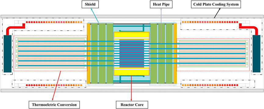
FIGURE 1. NUSTER-100 structure.

FIGURE 2

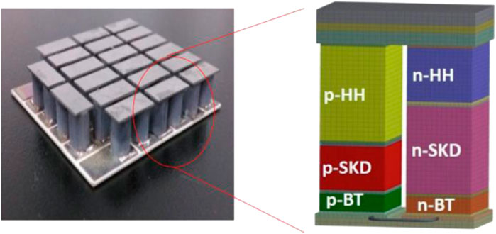
FIGURE 2. Thermoelectric converter schematic (Tang et al., 2022).

A nonlinear model for NUSTER-100 is necessary for control performance evaluation. The nonlinear model of NUSTER-100 can be divided into three parts: reactor core model, heat transfer model and thermoelectric conversion model.

2.1 Reactor core model

The core model of NUSTER-100 adopts a point reactor kinetics model with six groups of delayed neutrons, as shown in Eq. 1, where ρ(t) is the input of the nuclear reactor and n(t) is the output of the nuclear reactor (Zhang, 2014)

$\{\begin{array}{c}\frac{dn\left(t\right)}{dt}=\frac{\rho \left(t\right)-\beta }{\mathrm{\Lambda }}n\left(t\right)+{\displaystyle \sum }_{i=1}^6{\lambda }_j{c}_j\left(t\right)\\ \frac{d{c}_j\left(t\right)}{dt}=\frac{{\beta }_j}{\mathrm{\Lambda }}n\left(t\right)-{\lambda }_j{c}_j\left(t\right),j=\mathrm{1,2},\dots ,6\end{array}(1)$

where $\beta ={\sum }_{j=1}^6{\beta }_j$.

The reactivity is calculated by Eq. 2 and it includes the control rod reactivity, and temperature reactivity feedback from the fuel and matrix. Reactivity caused by fuel and matrix temperature changes are obtained by Eqs. 3, 4.

$\begin{array}{c}\rho ={\rho }_{rod}+{\rho }_{dop}+{\rho }_{Mo}(2)\\ {\rho }_{dop}={\alpha }_{dop}{T}_{fuel}-{\alpha }_{dop}{T}_{\left(fuel,100\right)}(3)\\ \begin{array}{c}{\rho }_{Mo}={\alpha }_{Mo}{T}_{Mo}-{\alpha }_{Mo}{T}_{\left(Mo,100\right)}(4)\end{array}\end{array}$

2.2 Heat transfer model

The heat transfer process can be divided into three stages: the first stage is from the fuel rod to the hot end of the heat pipe, the second stage is from the hot end of the heat pipe through the shielding area to the cold end of the heat pipe, and the third stage is from the cold end of the heat pipe to the collector.

For one single heat pipe, there are four fuel rods and one moderator rod surrounding the heat pipe as shown in Figure 3A. Using volume equivalence, the reactor core is simplified to a circular tube, as shown in Figure 3B. Using the lumped parameter method, the temperature of each material is concentrated on one temperature node and the model has eight temperature nodes, i.e., fuel, helium gap, cladding, substrate, heat pipe wall, liquid sodium, wick, and vapor sodium. In addition, heat conduction is considered to be axisymmetric and axial heat conduction is ignored Yang and Tao, (2006). This series of simplifications not only improve the efficiency of heat transfer calculations, but also preserve the overall characteristics of the heat transfer process and meet the requirements of control simulations.

FIGURE 3

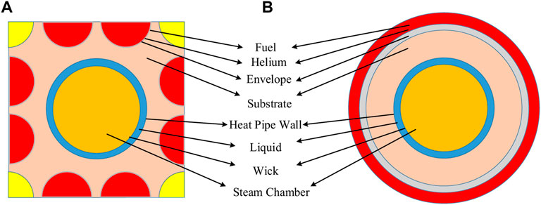
FIGURE 3. Revise the caption as comparison diagram of single-channel model (Pu et al., 2021): (A) Reactor core unit. (B) Reactor core single-channel model.

The ordinary differential equations to calculate the temperature of each node are derived through the Fourier law and the law of conservation of energy, which are shown as Eqs. 5, 6:

$\begin{array}{c}\dot{\Delta U}={\dot{Q}}_{out}+{\dot{Q}}_{in}(5)\\ \frac{d\left(m_i{C}_{p,i}{T}_i\right)}{dt}=K_{i-1_{-}i}\left(T_{i-1}-T_i\right)-K_{i_{-}i+1}\left(T_i-T_{i+1}\right)+Q_{in}(6)\end{array}$

When calculating the node temperature, the heat transfer coefficient between nodes is necessary, which can be obtained by Eq. 7:

$K_{i\_i+1}=\frac{1}{R_i+R_{i+1}}=\frac{1}{\frac{1}{2\pi {\lambda }_i\left(T_i\right)l_i}\mathit{ln}\left(\frac{d_i}{d_{i\_i+1}}\right)+\frac{1}{2\pi {\lambda }_{i+1}\left(T_{i+1}\right)l_{i+1}}\mathit{ln}\left(\frac{d_{i\_i+1}}{d_{i+1}}\right)}(7)$

where i represents the current node, i-1 represents the previous node, and i+1 represents the next node.

The second stage of the heat transfer model has two nodes, namely the shielding area and the condensation area. The calculation equation of each node temperature is the same as that of the first heat transfer model. The heat transfer coefficient between the nodes is:

$K=\lambda l(8)$

The third-stage heat transfer model has four nodes, namely the wick, liquid sodium, heat pipe wall, and collector. The transfer method of the temperature of each node is opposite to that of the first-stage heat transfer model, and the calculation method is the same, which is not repeated here.

2.3 Thermoelectric conversion model

The thermoelectric conversion model is more concerned with the temperature difference between the hot and cold ends. The main nodes are the copper plates at the hot end and the copper plate at the cold end of the thermoelectric converter. The ordinary differential equation for calculating the temperature of each node is shown in Eq. 6, and the heat transfer coefficient needs to be calculated using the thermal resistance network shown in Figure 4. The calculation is based on Eq. 9.

$K_{Cu\_Cuc}=\frac{1}{R_{Cu}+R_{P\_N}+R_{Cuc}}=\frac{1}{\frac{{\delta }_{Cu}}{{\lambda }_{Cu}{A}_{Cu}}+\frac{\frac{{\delta }_P}{{\lambda }_P{A}_P}\times \frac{{\delta }_N}{{\lambda }_N{A}_N}}{\frac{{\delta }_P}{{\lambda }_P{A}_P}+\frac{{\delta }_N}{{\lambda }_N{A}_N}}+\frac{{\delta }_{Cuc}}{{\lambda }_{Cuc}{A}_{Cuc}}}(9)$

FIGURE 4

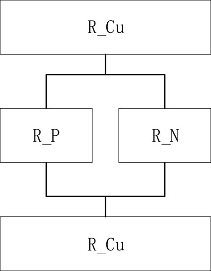
FIGURE 4. Thermoelectric converter equivalent thermal resistance network.

3 Linear dynamic model development

In Section 2, the nonlinear dynamic model of NUSTER-100 is established. Because the MPC controller needs a state space model of NUSTER-100 as the prediction model, the nonlinear model needs to be linearized to obtain its state space model. Linearization is carried out based on the perturbation theory (Tong et al., 2018). The equilibrium point is first selected, and a small disturbance is introduced at the equilibrium point to obtain the linear differential equation among the state variables of the system. The state space model of the system can be established through linear differential equations.

Take the reactor core model as an example and the linearization of the rest part is similar. Assume that at t₀ time, the nuclear reactor is in a steady state, and the steady state value of each state is n₀, c_j,0, ρ₀. If there is a small change Δρ in the reactivity at this time, there will also be a small change in the neutron density n and delayed neutron precursor concentration c. Thus, we can obtain ρ = ρ₀+Δρ, c_j = c_j,0+Δc_j.

At steady state, the total reactivity ρ = 0, the left-hand side of Eq. 1 is 0, the following relationships can be obtained:

$\{\begin{array}{c}\frac{{\beta }_j{n}_0}{\mathrm{\Lambda }}={\lambda }_j{c}_{j,o}\\ \frac{\beta n_0}{\mathrm{\Lambda }}={\displaystyle \sum }_{j=1}^6{\lambda }_j{c}_{j,o}\end{array}(10)$

Substituting Eq. 10 into Eq. 1, one can obtain:

$\{\begin{array}{c}\frac{\mathrm{d}\Delta n\left(t\right)}{\mathrm{d}t}=\frac{n_0}{\mathrm{\Lambda }}\Delta \rho \left(t\right)+\frac{\Delta \rho \left(t\right)}{\mathrm{\Lambda }}\Delta n\left(t\right)+\frac{{\rho }_0-\beta }{\mathrm{\Lambda }}\Delta n\left(t\right)+{\displaystyle \sum }_{j=1}^6{\lambda }_j\Delta c_j\left(t\right)\\ \frac{\mathrm{d}\Delta c_j\left(t\right)}{\mathrm{d}t}=\frac{{\beta }_j}{\mathrm{\Lambda }}\Delta n\left(t\right)-{\lambda }_j\Delta c_j\left(t\right),j=\mathrm{1,2},...,6\end{array}(11)$

The term $\frac{\Delta \rho \left(t\right)}{\mathrm{\Lambda }}\Delta n\left(t\right)$ is high-order infinitesimal and can be ignored. Thus, Eq. 11 can be transformed into linearized equations of dynamic equations:

$\begin{array}{c}\{\begin{array}{c}\frac{\mathrm{d}\Delta n\left(t\right)}{\mathrm{d}t}=\frac{n_0}{\mathrm{\Lambda }}\Delta \rho \left(t\right)+\frac{{\rho }_0-\beta }{\mathrm{\Lambda }}\Delta n\left(t\right)+{\displaystyle \sum }_{j=1}^6{\lambda }_j\Delta c_j\left(t\right)\\ \frac{\mathrm{d}\Delta c_j\left(t\right)}{\mathrm{d}t}=\frac{{\beta }_j}{\mathrm{\Lambda }}\Delta n\left(t\right)-{\lambda }_j\Delta c_j\left(t\right),j=\mathrm{1,2},...,6\end{array}\end{array}(12)$

Select $\begin{array}{c}{\mathit{x}}_1={\left[\Delta n\Delta c_1\Delta c_2\Delta c_3\Delta c_4\Delta c_5\Delta c_6\right]}^T\end{array}$ as the state vector, ${\mathit{u}}_1=\left[\Delta \rho \right]$ as the input variable, and ${\mathit{y}}_1=\left[\Delta n\right]$ as the output variable. Eq. 12 can be written as a state space model as shown in Eq. 13.

$\{\begin{array}{c}{\dot{\mathit{x}}}_1={\mathit{A}}_1{\mathit{x}}_1+{\mathit{B}}_1{\mathit{u}}_1\\ {\mathit{y}}_1={\mathit{C}}_1{\mathit{x}}_1+{\mathit{D}}_1{\mathit{u}}_1\end{array}(13)$

where, ${\mathit{A}}_1$, ${\mathit{B}}_1$, ${\mathit{C}}_1$, ${\mathit{D}}_1$ are as follows:

${\mathit{A}}_1=\left[\begin{array}{ccccccc}\frac{{\rho }_0-\beta }{\mathrm{\Lambda }}& {\lambda }_1& {\lambda }_2& {\lambda }_3& {\lambda }_4& {\lambda }_5& {\lambda }_6\\ \frac{{\beta }_1}{\mathrm{\Lambda }}& -{\lambda }_1& 0& 0& 0& 0& 0\\ \frac{{\beta }_2}{\mathrm{\Lambda }}& 0& -{\lambda }_2& 0& 0& 0& 0\\ \frac{{\beta }_3}{\mathrm{\Lambda }}& 0& 0& -{\lambda }_3& 0& 0& 0\\ \frac{{\beta }_4}{\mathrm{\Lambda }}& 0& 0& 0& -{\lambda }_4& 0& 0\\ \frac{{\beta }_5}{\mathrm{\Lambda }}& 0& 0& 0& 0& -{\lambda }_5& 0\\ \frac{{\beta }_6}{\mathrm{\Lambda }}& 0& 0& 0& 0& 0& -{\lambda }_6\end{array}\right]{\mathit{B}}_1=\left[\begin{array}{c}\frac{n_0}{\mathrm{\Lambda }}\\ 0\\ 0\\ 0\\ 0\\ 0\\ 0\end{array}\right]{\mathit{C}}_1=\left[\begin{array}{ccccccc}1& 0& 0& 0& 0& 0& 0\end{array}\right]{\mathit{D}}_1=\left[0\right]$

Similarly, the state space models of the heat transfer model and the thermoelectric conversion model can be obtained. Connect the state space models of the reactor core model, heat transfer model, and thermoelectric conversion model. The state space model of NUSTER-100 can be obtained as Eq. 14.

$\{\begin{array}{l}\dot{\mathit{x}}={\mathit{A}}_c\mathit{x}+{\mathit{B}}_c\mathit{u}\\ \mathit{y}={\mathit{C}}_c\mathit{x}\end{array}(14)$

where, the state vector x, the input variable u, the output variable y are as follows:

$\mathit{x}={\left[\begin{array}{c}\Delta n\Delta c_1\Delta c_2\Delta c_3\Delta c_4\Delta c_5\Delta c_6\end{array}{T}_{fuel}{T}_{Clad}{T}_{Mo}{T}_{\mathrm{W}\mathrm{a}\mathrm{l}\mathrm{l}}{T}_{N{a}_{-}l}{T}_{\mathrm{W}\mathrm{i}\mathrm{c}\mathrm{k}}{T}_{N{a}_{-}v}{T}_{Sc}{T}_{N{a}_{-}vc}{T}_{Wickc}{T}_{N{a}_{-}lc}{T}_{Wallc}{T}_{Sur}{T}_{Cu}{T}_{Cuc}\right]}^{\mathrm{T}}\mathit{u}=\left[\Delta \rho \right]\mathit{y}=\left[\Delta P_{elec}\right]$

4 The principles of MPC

MPC is an advanced control strategy, which uses the plant model and the feedback measurements of the current process to calculate the future control value while satisfying constraints. The calculated control value is output to the controlled object to realize the control effect.

MPC obtains the control value u(k) by solving the optimization problem. The output y(k) of controlled object is sent to the model predictive controller as a feedback for the next step of optimization. Each round of optimization obtains the optimal output increment based on the prediction model, the reference trajectory and the output value at the current moment. MPC is mainly composed of prediction model, rolling optimization and feedback correction (Wang et al., 2017), and its structure is shown in Figure 5.

FIGURE 5

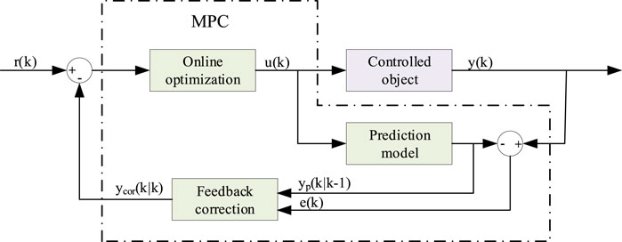
FIGURE 5. MPC structure.

4.1 Prediction model

MPC is a model-based control algorithm and a prediction model is used. The function of the prediction model is to predict the future output of controlled object based on its historical information and future inputs. The specific expression form of this model is not important, and the important part is that it can realize the prediction function. The state space model of NUSTER-100 is obtained and selected as the prediction model in this study. The continuous state space model needs to be discretized to implement the controller (Eq. 15):

$\{\begin{array}{l}\dot{\mathit{x}}\left(k+1\right)={\mathit{A}}_d\mathit{x}\left(k\right)+{\mathit{B}}_d\mathit{u}\left(k\right)\\ \mathit{y}\left(k+1\right)={\mathit{C}}_d\mathit{x}\left(k+1\right)\end{array}(15)$

where, ${\mathit{A}}_d={\mathrm{e}}^{{\mathit{A}}_c{T}_s}$, ${\mathit{B}}_d={\int }_0^{T_s}{\mathrm{e}}^{{\mathit{A}}_{\mathit{c}}\tau }\cdot {\mathit{B}}_c\mathrm{d}\tau$, ${\mathit{C}}_d={\mathit{C}}_c$, T_s is the sampling time.

In order to facilitate the solution of the control variables, the discrete state space model is rewritten as an incremental model (Chen, 2013), as shown in Eq. 16.

$\{\begin{array}{c}\Delta \mathit{x}\left(k+1\right)={\mathit{A}}_d\Delta \mathit{x}\left(k\right)+{\mathit{B}}_d\Delta \mathit{u}\left(k\right)\\ \mathit{y}\left(k+1\right)={\mathit{C}}_d\Delta \mathit{x}\left(k+1\right)+\mathit{y}\left(k\right)\end{array}(16)$

where,

$\{\begin{array}{l}\Delta \mathit{x}\left(k\right)=\mathit{x}\left(k\right)-\mathit{x}\left(k-1\right)\\ \Delta \mathit{u}\left(k\right)=\mathit{u}\left(k\right)-\mathit{u}\left(k-1\right)\end{array}$

In order to derive the predictive equation from the prediction model, let the prediction horizon be p and the control horizon be m and m ≤ p. At the current moment k, taking the measured value of state variable x(k) as the starting point, the state value at any time in the horizon p can be predicted by recursive operation of the system equation of the incremental model (Eq. 16), as shown in Eqs. 17, 18.

$\begin{array}{c}\begin{array}{cc}\Delta \mathit{x}\left(k+i|k\right)={{\mathit{A}}_d}^i\Delta \mathit{x}\left(k\right)+{{\mathit{A}}_d}^{i-1}{\mathit{B}}_d\Delta \mathit{u}\left(k\right)+{{\mathit{A}}_d}^{i-2}{\mathit{B}}_d\Delta \mathit{u}\left(k+1\right)& +\cdots +{\mathit{B}}_d\Delta \mathit{u}\left(k+i-1\right),i=\mathrm{1,2},...,m(17)\end{array}\\ \begin{array}{cc}\Delta \mathit{x}\left(k+j|k\right)={{\mathit{A}}_d}^j\Delta \mathit{x}\left(k\right)+{{\mathit{A}}_d}^{j-1}{\mathit{B}}_d\Delta \mathit{u}\left(k\right)+{{\mathit{A}}_d}^{j-2}{\mathit{B}}_d\Delta \mathit{u}\left(k+1\right)& +\cdots +{{\mathit{A}}_d}^{j-m}{\mathit{B}}_d\Delta \mathit{u}\left(k+m-1\right),j=m+1,...,p\end{array}\end{array}(18)$

where, k + i | k indicates the state predicted value of the time k + i at the time k. When the time exceeds m, the change of corresponding control variable is equal to 0.

The output equation of the prediction model Eq. 15 can predict the system output, that is electric power $P_{elec}$. For the convenience of analysis, the prediction output vector and control vector are defined as follows:

$\begin{array}{c}{\mathit{Y}}_{\mathit{p}}\left(k+1|k\right)\stackrel{\mathrm{def}}{=}\left[\begin{array}{c}{\mathit{y}}_{\mathit{p}}\left(k+1|k\right)\\ {\mathit{y}}_{\mathit{p}}\left(k+2|k\right)\\ ⋮\\ {\mathit{y}}_{\mathit{p}}\left(k+p|k\right)\end{array}\right]\end{array}\mathit{U}\left(k\right)\stackrel{\mathrm{def}}{=}\left[\begin{array}{c}\mathit{u}\left(k\right)\\ \mathit{u}\left(k+1\right)\\ ⋮\\ \mathit{u}\left(k+m-1\right)\end{array}\right]$

The predicted value in the prediction time horizon can be calculated by the following prediction equation:

$\begin{array}{c}{\mathit{Y}}_p\left(k+1|k\right)={\mathit{\Phi }}_x\mathit{x}\left(k\right)+{\mathit{I}}_y\mathit{y}\left(k\right)+{\mathit{\Phi }}_u\mathit{U}\left(k\right)\end{array}(19)$

where,

${\mathit{I}}_y={\left[\begin{array}{c}1\\ 1\\ ⋮\\ 1\end{array}\right]}_{p\times 1},\begin{array}{c}{\mathit{\Phi }}_x=\left[\begin{array}{c}{\mathit{C}}_d{\mathit{A}}_d\\ {\displaystyle \sum }_{i=1}^2{\mathit{C}}_d{{\mathit{A}}_d}^i\\ ⋮\\ {\displaystyle \sum }_{i=1}^{\mathit{p}}{\mathit{C}}_d{{\mathit{A}}_d}^i\end{array}\right]\end{array},{\mathit{\Phi }}_u=\left[\begin{array}{ccccc}{\mathit{C}}_d{\mathit{B}}_d& \mathbf{0}& \mathbf{0}& \cdots & \mathbf{0}\\ {\displaystyle \sum }_{i=1}^2{\mathit{C}}_d{{\mathit{A}}_d}^{i-1}{\mathit{B}}_d& {\mathit{C}}_d{\mathit{B}}_d& \mathbf{0}& \cdots & \mathbf{0}\\ ⋮& ⋮& ⋮& \ddots & ⋮\\ {\displaystyle \sum }_{i=1}^m{\mathit{C}}_d{{\mathit{A}}_d}^{i-1}{\mathit{B}}_d& {\displaystyle \sum }_{i=1}^{m-1}{\mathit{C}}_d{{\mathit{A}}_d}^{i-1}{\mathit{B}}_d& \cdots & \cdots & {\mathit{C}}_d{\mathit{B}}_d\\ ⋮& ⋮& ⋮& \ddots & ⋮\\ {\displaystyle \sum }_{i=1}^p{\mathit{C}}_d{{\mathit{A}}_d}^{i-1}{\mathit{B}}_d& {\displaystyle \sum }_{i=1}^{p-1}{\mathit{C}}_d{{\mathit{A}}_d}^{i-1}{\mathit{B}}_d& \cdots & \cdots & {\displaystyle \sum }_{i=1}^{p-m+1}{\mathit{C}}_d{{\mathit{A}}_d}^{i-1}{\mathit{B}}_d\end{array}\right]$

4.2 Feedback correction

Since the controlled object is a nonlinear system, the predicted value based on its linear model cannot be completely consistent with the actual system output. Therefore, it is necessary to use the deviation between the predicted value at the previous time y_p (k|k-1) and the measured value at the current time y(k) to perform feedback correction on the predicted value at the current moment, as shown in Eq. 20:

$\begin{array}{ll}{\mathit{Y}}_{cor}\left(k+1|k\right)={\mathit{Y}}_p\left(k+1|k\right)+\mathit{H}\left[y\left(k\right)-y_p\left(k|k-1\right)\right]& ={\mathit{Y}}_p\left(k+1|k\right)+\mathit{H}e\left(k\right)\end{array}(20)$

where $\mathit{H}={\left[h\left(1\right)\cdots h\left(p\right)\right]}^T$ is the error correction matrix.

The correction value Y_cor (k+1|k) with error information is used to carry out a new round of optimization. The error information will be considered when solving the new control variable, so as to realize feedback correction.

4.3 Rolling optimization

MPC is an optimization control algorithm that obtains future control value by solving optimization problem. Furthermore, compared with optimal control, the optimization in MPC is a rolling optimization with a limited period of time. At current sampling moment, the optimal solution of the optimization problem only involves a limited time in the future from that moment. At the next sampling moment, the optimization period moves forward. Therefore, the relative form of the optimization problem at different time is the same while its absolute form, that is, the time area included, is different (Bemporad and Morari, 1999).

4.3.1 Optimization problem

In this study, the optimization problem is set as the difference between the measured value and the reference trajectory, and the change rate limit of the control variable. Moreover, the importance of the index can be adjusted by the weight of each index, as shown in Eq. 21.

$\begin{array}{c}\min J={\displaystyle \sum }_{i=1}^p{\Vert {\gamma }_y\left(y\left(k+i|k\right)-r\left(k+i\right)\right)\Vert }^2+{\displaystyle \sum }_{i=1}^m{\Vert {\gamma }_u\Delta u\left(k+i-1\right)\Vert }^2\end{array}(21)$

The matrix-vector form is:

$\begin{array}{c}\min J={\Vert {\mathit{\Gamma }}_y\left({\mathit{Y}}_{cor}\left(k+1|k\right)-\mathit{R}\left(k+1\right)\right)\Vert }^2+{\Vert {\mathit{\Gamma }}_u\Delta \mathit{U}\left(k\right)\Vert }^2\end{array}(22)$

where ${\mathit{\Gamma }}_y$, ${\mathit{\Gamma }}_u$ is the weight matrix, as shown in Eq. 23 Compared with the weight factor ${\gamma }_y$, ${\gamma }_u$, a larger weight value imposes a higher penalty on its associated performance factor by increasing its contribution to the optimization problem.

$\{\begin{array}{l}{\mathit{\Gamma }}_y=diag{\left({\gamma }_y\right)}_{p\times p}\\ {\mathit{\Gamma }}_u=diag{\left({\gamma }_u\right)}_{m\times m}\end{array}(23)$

4.3.2 Optimization problem solution

According to the objective function, let

$\frac{\partial J\left(\Delta U\right)}{\partial \Delta U}=0(24)$

Substituting Eqs. 19, 20, the optimal control sequence at time $k$ can be obtained:

$\begin{array}{c}\Delta {\mathit{U}}^{*}\left(k\right)={\left({\mathit{\Phi }}_u^{\mathrm{T}}{\mathit{\Gamma }}_y^{\mathrm{T}}{\mathit{\Gamma }}_y{\mathit{\Phi }}_u+{\mathit{\Gamma }}_u^{\mathrm{T}}{\mathit{\Gamma }}_u\right)}^{-1}{\mathit{\Phi }}_u^{\mathrm{T}}{\mathit{\Gamma }}_y^{\mathrm{T}}{\mathit{\Gamma }}_y{\mathit{E}}_p\left(k+1|k\right)\end{array}(25)$

where E_p (k+1|k) is error and shown in Eq. 26.

$\begin{array}{c}{\mathit{E}}_p\left(k+1|k\right)=\mathit{R}\left(k+1\right)-{\mathit{\Phi }}_x\Delta \mathit{x}\left(k\right)-{\mathit{I}}_y\end{array}\mathit{y}\left(k\right)-\mathit{H}e\left(k\right)(26)$

Eq. 25 is the optimal solution of the control variable increment in the control time horizon. To prevent the error of control from the ideal state caused by model mismatch or environmental disturbance, only the first increment of the control variable increment sequence is acted on the system. The control increment acting on the system in real time is:

$\begin{array}{ll}\begin{array}{c}\Delta u\left(k\right)={\left[\begin{array}{cccc}1& \mathbf{0}& \cdots & \mathbf{0}\end{array}\right]}_{1\times m}\Delta U^{*}\left(k\right)\end{array}& ={\left[\begin{array}{cccc}1& \mathbf{0}& \cdots & \mathbf{0}\end{array}\right]}_{1\times m}{\left({\mathit{\Phi }}_u^{\mathrm{T}}{\mathit{\Gamma }}_y^{\mathrm{T}}{\mathit{\Gamma }}_y{\mathit{\Phi }}_u+{\mathit{\Gamma }}_u^{\mathrm{T}}{\mathit{\Gamma }}_u\right)}^{-1}{\mathit{\Phi }}_u^{\mathrm{T}}{\mathit{\Gamma }}_y^{\mathrm{T}}{\mathit{\Gamma }}_y{\mathit{E}}_p\left(k+1|k\right)\end{array}(27)$

The predictive control gains are defined as

${\mathit{K}}_{mpc}={\left[\begin{array}{cccc}1& \mathbf{0}& \cdots & \mathbf{0}\end{array}\right]}_{1\times m}{\left({\mathit{\Phi }}_u^{\mathrm{T}}{\mathit{\Gamma }}_y^{\mathrm{T}}{\mathit{\Gamma }}_y{\mathit{\Phi }}_u+{\mathit{\Gamma }}_u^{\mathrm{T}}{\mathit{\Gamma }}_u\right)}^{-1}{\mathit{\Phi }}_u^{\mathrm{T}}{\mathit{\Gamma }}_y^{\mathrm{T}}{\mathit{\Gamma }}_y(28)$

Then the control action can be calculated by the following equation:

$\begin{array}{ll}u\left(k\right)=u\left(k-1\right)+\Delta u\left(k\right)& =u\left(k-1\right)+{\mathit{K}}_{mpc}{\mathit{E}}_p\left(k+1|k\right)\end{array}(29)$

5 Power control system based on MPC

The power control system of NUSTER-100 based on MPC is designed using the linear model and the performance of the control system is verified on the nonlinear model. NUSTER-100 power control system is shown in Figure 6. The purpose of the control system is to maintain the electric power at the setpoint, and the measured value of the electric power needs to be fed back to the model predictive controller to form a closed-loop system. The output by the controller is the control rod reactivity.

FIGURE 6

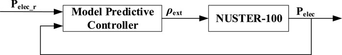
FIGURE 6. NUSTER-100 electric power control system.

Next, the parameters of the MPC controller need to be set. A -10pcm step disturbance with the open-loop system is performed on the controlled object NUSTER-100, and the electric power response is shown in Figure 7. The rise time Tr is around 42.44s, and the sample time of the controller is set to T_r/20≈2s. To cover the significant dynamics of the open-loop system, the prediction horizon p is set to 30. To balance control effects and computational complexity, a good rule of thumb for choosing the control horizon is to set it as 10%–20% of the prediction horizon (Bemporad et al., 2020). Here it is set as 5. Since the difference in the order of magnitude between electric power and control rod reactivity is 10^–5, the output weight of the controlled object ${\gamma }_y$ is set to 10^–4, and the weight of the control variable rate of change ${\gamma }_u$ is set to 0.1. At the same time, considering the mechanical limit of the control rod drive mechanism, the output change rate of the controller is limited to -10^–5∼10^–5.

FIGURE 7

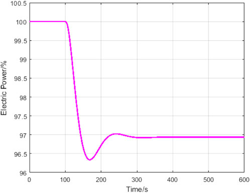
FIGURE 7. Electric power response to reactivity step disturbance.

A -10% step change in the electric power setpoint is introduced to evaluate the control performance. The simulation starts from 0s at 100%FP, and at 100s the setpoint is changed stepwise from 100% to 90%. Simulations are performed in MATLAB and Simulink environment.

The system responses are shown in Figure 8. At 100s, the controller starts to act due to the error signal. The control rod reactivity is introduced at a certain rate due to mechanical constraints and stabilizes at 3.2 × 10^–4 after 150s (Figure 8A). As shown in Figure 8B, due to the introduction of negative reactivity, the core power is rapidly reduced to 85.9%. As a results, the fuel temperature changes (Figure 8C), and the fuel temperature change in turn causes the neutron resonance absorption rate to change, resulting in reactivity feedback (Figure 8D). The core power gradually increases and stabilizes at 94%. Because the heat transfer process of the heat pipe has a certain delay, the hot end temperature of the thermoelectric conversion device does not respond promptly to the change of the control rod reactivity, and drops to 993K relatively slowly (Figure 8E). With the change of the hot end temperature of the thermoelectric conversion device, the electric power gradually decreases and stabilizes at 90.3%, with a steady-state error of 0.3% (Figure 8F).

FIGURE 8

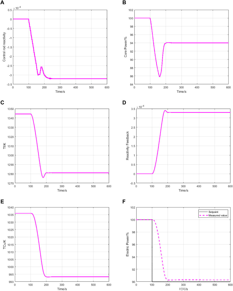
FIGURE 8. System response under MPC controller: (A) Control rod reactivity response. (B) Core power response. (C) Fuel temperature response. (D) reactivity feedback response. (E) Thermoelectric conversion device hot end temperature response. (F) Electric power response.

The steady-state error cannot be eliminated by only modifying the controller parameters. Therefore, the structure of the control system is modified, and an integral controller is introduced. MPC controller with an Integral controller to eliminate steady state error is named as IMPC in this study. The modified block diagram of IMPC is shown in Figure 9.

FIGURE 9

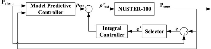
FIGURE 9. NUSTER-100 power control system with IMPC.

To reduce overshoot, a selector is added in front of the integral controller. The function of the selector is that when the absolute value of the error e is greater than the threshold e_h, the selector outputs e' = 0, otherwise, e' = e, as shown in Eq. 30. Using the selector, the error integral controller can only play a role when the error is small, so as to achieve the control effect of eliminating the steady-state error without increasing the overshoot.

$\{\begin{array}{l}{e}^{\prime }=e,e\le e_h\\ e^{\prime }=0,e>e_h\end{array}(30)$

After parameter tuning experiments based on trial and error method, the integral coefficient is set to be 6 × 10^–7, and the threshold e_h is set as 4. The parameters of the MPC controller remain unchanged. For comparison, a PI controller is also formulated for NUSTER-100 as shown in Figure 10. The parameters of PI controller are tuned through a tuning technique based on genetic algorithm (Mantri and Kulkarni., 2013). The proportional coefficient is 1.05 × 10^–8, and the integral coefficient is 5.45 × 10^–7.

FIGURE 10

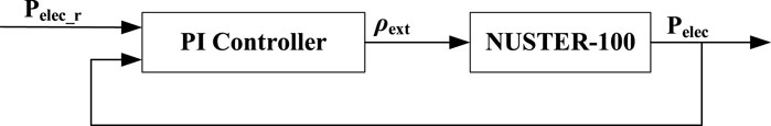
FIGURE 10. NUSTER-100 power control system with PI controller.

In order to evaluate the control performance, simulations under various typical operating conditions are carried out. The first case, a 10% step change in the electric power setpoint is introduced. The simulation starts from 0s at 100%FP, and at 100s the setpoint is changed stepwise from 100% to 90%. The system responses are shown in Figure 11. PI, MPC and IMPC stand for the results with PI controller, MPC controller and IMPC controller, respectively. During the 0–100s of the simulation, all parameters are kept as the initial values. At 100s, the electric power setpoint is changed. As shown in Figure 11A, the overall change trend of the control rod reactivity is decreasing. As shown in Figure 11B, the core power rapidly decreases to the lowest point, then increases rapidly and reaches a steady state. As shown in Figures 11C,D, the thermoelectric conversion device hot end temperature and electric power have similar trends. They both decrease monotonically and reach a steady state smoothly. Under the regulation of PI controller and IMPC controller, the electric power successfully reaches the setpoint, while under the regulation of MPC controller, the electric power has one steady-state error.

FIGURE 11

FIGURE 11. System responses under IMPC controller and PI controller in case 1: (A) Control rod reactivity response. (B) Core power response. (C) Thermoelectric conversion device hot end temperature response. (D) Electric power response.

The second case, a -2%FP/min ramp change in the electric power setpoint is introduced. The simulation starts from 0s at 100%FP, and at 100s the setpoint is linearly changed from 100% to 90%FP. The system responses are shown in Figure 12. As the setpoint of the electric power decreases linearly, the parameters of the system also decrease gradually and reach a steady state. As shown in Figure 12D, under the regulation of PI controller and IMPC controller, the electric power successfully reaches the setpoint, while under the regulation of MPC controller, the electric power has steady-state error. Moreover, it can be seen that the IMPC control system can track the change of the electric power setpoint more quickly than the PI control system.

FIGURE 12

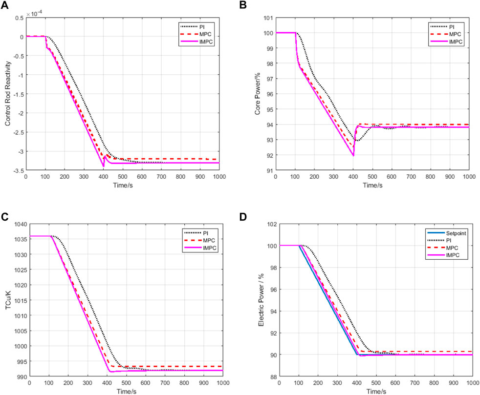
FIGURE 12. System response under IMPC controller and PI controller in case 2: (A) Control rod reactivity response. (B) Core power response. (C) Thermoelectric conversion device hot end temperature response. (D) Electric power response.

The third case is similar to the second case. The simulation starts from 0s at 100%FP, and at 100s the setpoint is linearly changed from 100% to 50%FP. As shown in Figure 13. the system responses are also similar to the second case, indicating that the system can achieve a wide range of power regulation.

FIGURE 13

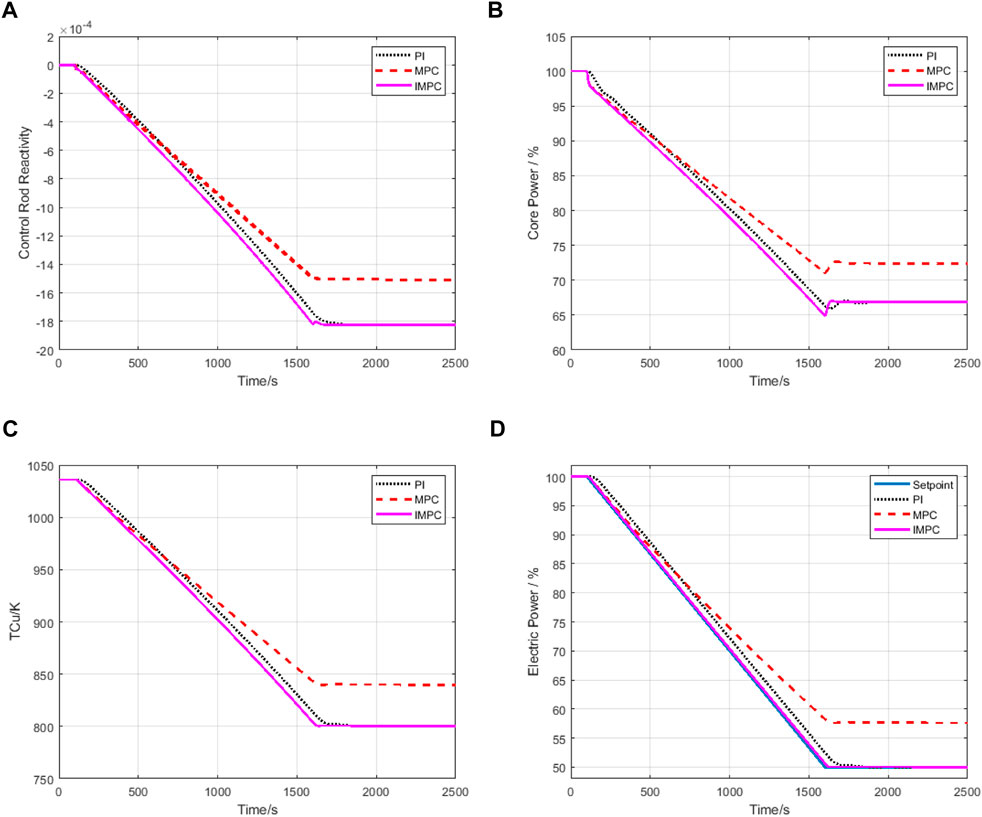
FIGURE 13. System response under IMPC controller and PI controller in case 3: (A) Control rod reactivity response. (B) Core power response. (C) Thermoelectric conversion device hot end temperature response. (D) Electric power response.

As shown in Table 1, using the IMPC controller, the electric power can track the setpoint changes more quickly than using PI controller. At the same time, the problem of steady-state error of MPC controller is effectively solved by adding the integral controller.

TABLE 1

TABLE 1. Transient performance.

6 Conclusion

In this study, in order to improve the response speed of the heat pipe cooled reactor system and enable the electric power of heat pipe cooled reactor to track the change of the setpoint faster, an MPC strategy with an integral controller is proposed for the electric power control of HPR. The MPC controller uses the linearized model of the controlled object as the predictive model, and obtains the control variable by solving the optimization problem to achieve the control effect. In order to eliminate the steady-state error, the proposed control scheme adds an integral controller with a selector.

To verify the performance of the controller, a marine silent HPR, NUSTER-100, is taken as the controlled object, and simulation tests are carried out. As demonstrated by simulations, the proposed controller provides enhanced control performance with improved speed under different operating conditions. Compared with the traditional PI controller and MPC controller, the system responds faster, and can track the change of the electric power setpoint faster with zero steady state error in various tests under the regulation of the proposed controller. The proposed controller provides a feasible method to improve the control performance of the HPR.

Data availability statement

The raw data supporting the conclusions of this article will be made available by the authors, without undue reservation.

Author contributions

JH: design of methodology, experimental data analysis, writing-original draft. PS: writing-review and editing, supervision, funding acquisition. SP: creation of model.

Funding

This paper is supported by the National Key Research and Development Program of China (No.2019YFB1901100).

Conflict of interest

The authors declare that the research was conducted in the absence of any commercial or financial relationships that could be construed as a potential conflict of interest.

Publisher’s note

All claims expressed in this article are solely those of the authors and do not necessarily represent those of their affiliated organizations, or those of the publisher, the editors and the reviewers. Any product that may be evaluated in this article, or claim that may be made by its manufacturer, is not guaranteed or endorsed by the publisher.

References

Bemporad, A., Morari, M., and Ricker, N. L. (2010). Model predictive control toolbox user’s guide. Natick: The mathworks.

Google Scholar

Bemporad, A., and Morari, M. (1999). “Robust model predictive control: A survey,” in Robustness in identification and control (London: Springer), 207–226.

Google Scholar

Bobal, V., Kubalcik, M., Dostal, P., and Matejicek, J. (2013). Adaptive predictive control of time-delay systems. Comput. Math. Appl. 66 (2), 165–176. doi:10.1016/j.camwa.2013.01.035

CrossRef Full Text | Google Scholar

Bone, V., Kearney, M., and Jahn, I. (2021). Towards model predictive control of supercritical CO2 cycles. https://arxiv.org/abs/2108.12127.

Google Scholar

Chen, H. (2013). Model predictive control. Beijing: Science Press.

Google Scholar

Chen, Q. (2011). Research of predictive control in the large time delay system. Hangzhou, China. Hangzhou Dianzi University.

Google Scholar

Eliasi, H., Davilu, H., and Menhaj, M. B. (2007). Adaptive fuzzy model based predictive control of nuclear steam generators. Nucl. Eng. Des. 237 (6), 668–676. doi:10.1016/j.nucengdes.2006.08.007

CrossRef Full Text | Google Scholar

Jiang, D., Liu, X., and Kong, X. (2019). Soft constrained MPC on water level control in steam generator of a nuclear power plant. Acta Autom. Sin. 45 (6), 1111–1121.

Google Scholar

Li, Y., Shen, J., and Zhang, J. (September 2019). Research on pressure and water level control of the pressurizer for marine nuclear power plant based on multivariable MPC, Proceedings of the 2019 4th international conference on power and renewable energy (ICPRE), power and renewable energy (ICPRE), Chengdu, China. 284–289.

Google Scholar

Mantri, G., and Kulkarni, N. R. (2013). Design and optimization of PID controller using genetic algorithm. Int. J. Res. Eng. Technol. 2 (6), 926–930. doi:10.15623/ijret.2013.0206002

CrossRef Full Text | Google Scholar

Pu, S., Sun, A., Sun, P., and Wei, X. (April 2022). “Reactor power robust control for a heat pipe cooled reactor,” in Proceedings of the International Symposium on Software Reliability, Industrial Safety, Cyber Security and Physical Protection for Nuclear Power Plant (Singapore: Springer), 399–410.

Google Scholar

Pu, S., Sun, P., and Wei, X. (2021). Transfer function development and dynamic analysis of a heat pipe. Cool. React. 4. Student Paper Competition.

Google Scholar

Tang, S., Liu, X., WangWang, C., Zhang, D., Su, G., Tian, W., et al. (2022). Thermal-electrical coupling characteristic analysis of the heat pipe cooled reactor with static thermoelectric conversion. Ann. Nucl. Energy 168, 108870. doi:10.1016/j.anucene.2021.108870

CrossRef Full Text | Google Scholar

Tong, X., Zhang, L., and Wang, N. (2018). Research on model predictive control in purely lagging objects. Electron. Meas. Technol. 41 (23), 12–16.

Google Scholar

Wang, G., Wu, J., Zeng, B., Xu, Z., Wu, W., and Ma, X. (2017). Design of a model predictive control method for load tracking in nuclear power plants. Prog. Nucl. Energy 101, 260–269. doi:10.1016/j.pnucene.2017.08.012

CrossRef Full Text | Google Scholar

Yang, S., and Tao, W. (2006). Heat transfer. Beijing: Higher Education Press.

Google Scholar

Yu, H., Ma, Y., Zhang, Z., and Chai, X. (2019). Initiation and development of heat pipe cooled reactor. Nucl. Power Eng. 40 (4), 1–8.

Google Scholar

Zhang, J. (2014). Nuclear reactor control. Beijing: China Atomic Energy Press.

Google Scholar

Zhang, X., Sun, H., Sun, P., Huang, J., and Wei, X. (2022). “Control strategy study for a heat pipe cooled nuclear reactor. Available at SSRN 4214471.0L.

Google Scholar

Zhang, Z., Chai, X., Wang, C., Sun, H., Zhang, D., Tian, W., et al. (2021). Numerical investigation on startup characteristics of high temperature heat pipe for nuclear reactor. Nucl. Eng. Des. 378, 111180. doi:10.1016/j.nucengdes.2021.111180

CrossRef Full Text | Google Scholar

Nomenclature

n Neutron density(m⁻³)

ρ Reactivity(pcm)

β_j The delayed neutron fraction of the jth group

Λ Generation time(s)

λ_j The delayed neutron precursor decay constant of the jth group (s⁻¹)

c_j The delayed precursor nucleus density of the jth group (m⁻³)

Q_out External heat source(W)

Q_in Internal heat source(W)

m Mass(kg)

C_p Specific heat capacity at constant pressure (J∙kg⁻¹∙K⁻¹)

T Temperature(K)

K_i Heat transfer coefficient of ith node(W∙K⁻¹)

R Thermal resistance(K∙W⁻¹)

l Length(m)

δ Thickness(m)

A Area(m²)

A State matrix

B Input-state matrix

C Output-state matrix

D Feedforward matrix

P_elec Electric power(W)

Subscripts

rod Control rod

dop Doppler

Mo Matrix

fuel Fuel

Clad Cladding

Wall Heat pipe wall at the hot end

Na_l Liquid sodium at the hot end

Wick Wick at the hot end

Na_v Vapor sodium at the hot end

Sc Shield

Na_vc Vapor sodium at the cold end

Wickc Wick at the cold end

Na_lc Liquid sodium at the cold end

Wallc Heat pipe wall at the cold end

Sur Heat collector

Cu Hot end of thermoelectric conversion device

Cuc Cold end of thermoelectric conversion device