Mechanical characteristics and damage evolution of granite under freeze–thaw cycles

Rocks in cold regions experience freeze–thaw (F–T) cycles, which have a significant impact on their mechanical properties, causing a series of engineering challenges that threaten engineering stability. To investigate the mechanical characteristics and damage evolution of granite under the influence of F–T cycles, the microstructural evolution and macroscopic mechanical properties of granite were analyzed by conducting P-wave velocity tests, computed tomography scanning, and uniaxial compression tests subjected to different F–T cycles. The results revealed the following: 1) the number of F–T cycles and saturated water content significantly impact on the mechanical properties of granite; 2) as the number of F–T cycles increases, the P-wave velocity, peak strength, elastic modulus, and coefficient of frost resistivity of granite gradually decrease, but the F–T damage values increase; 3) when the number of F–T cycles is less than 40 but within a certain range (0–100), the damage variable of granite increases rapidly, but then gradually tends to stabilize; 4) the damage gradually steadily spreads to the central region of the granite sample as the number of F–T cycles increases, and the ends and marginal regions of the granite samples are more susceptible to damage, and 5) three damage variables with different definitions (elastic modulus, density, and porosity) can be used to predict the degree of damage of granite under F–T cycles.

1 Introduction

In recent years, with the development in the mining of mineral resources and the construction of infrastructure, such as open-pit mining, tunnel excavation, and highway and railway construction, have gradually extended to high-cold and high-altitude regions (Chang et al., 2018; Shen et al., 2018; Fan et al., 2020). The rock slopes of open-pit mining are severely affected by cyclic freeze–thaw (F–T) actions (the alternating freezing and thawing of water in rocks) in cold regions (Jamshidi et al., 2013; Huang et al., 2019, 2022). The F–T actions cause microcracks in rocks in alpine regions, resulting in rock strength degradation and frost heaving deformation. These cause rock slope instability, denudation, slump, and other engineering challenges, which pose a threat to human life and engineering stability (Li et al., 2014). The F–T damage in rocks is mainly caused by an approximately 9% volumetric expansion of freezing water inside pores, cracks, and joints, stressing the surrounding rocks upon freezing; this phenomenon leads to rocks deterioration (Hori and Morihiro, 1998; Park et al., 2015; Huang et al., 2020). Therefore, the influence of F–T cycles on the mechanical characteristics of rocks is important in geotechnical engineering in cold regions, and the damage evolution of rocks under F–T cycles should be explored.

In previous studies, the physical-mechanical properties of rocks under F–T cycles have been investigated from both micro- and macro-perspectives. In macroscopic analyses, the changing trends of a rock’s strength, porosity, stress-strain properties, and elastic modulus were analyzed by conducting uniaxial and triaxial tests, which mainly involved computed tomography (CT) scanning, nuclear magnetic resonance (NMR), and scanning electron microscopy (SEM), to observe the evolution of the internal structure of rocks under different numbers of F–T cycles. Numerous researchers have shown that with an increase in the number of F–T cycles, the P-wave velocity, compressive strength, elastic modulus, and weathering degree of rocks gradually decrease, whereas the porosity, water absorption, total strain energy, elastic energy, and dissipated energy of rocks gradually increase (Remy et al., 1994; Martínez-Martínez et al., 2013; Ghobadi and Babazadeh, 2015; Momeni et al., 2016; Mu et al., 2017; Gao et al., 2020). Temperature, rock type, water content, and number of F–T cycles were important factors that affect the physical and mechanical properties of rocks (Nicholson et al., 2000; Chen et al., 2004). Other researchers have investigated damage evolution, deterioration mechanisms of rock pore structures, pore structure distribution, and crack propagation in rocks during freezing and thawing using CT, NMR, and SEM (Yang et al., 1998; Martínez-Martínez et al., 2013; Park et al., 2015; Jia et al., 2020.; Liu et al., 2020; Sun et al., 2020). Based on the test results of rocks undergoing F–T cycles, a mathematical model (Mutluturk et al., 2004; Liu et al., 2015; Lu et al., 2019), index decay model (Mutlutürk et al., 2004), statistical model (Bayram, 2012), poro-elastic-plastic model (Liu et al., 2018), and elastoplastic micromechanical model (Huang et al., 2020) have been established to describe the deteriorating effects of the F–T actions on the mechanical properties of rocks.

Although the physical-mechanical properties and damage models of rocks under cyclic F–T actions have been extensively studied, only a few studies have been conducted on the mechanical characteristics and damage evolution of rocks under F–T cycles using a combination of micro- and macro-methods. Therefore, in this study, a series of P-wave velocity tests, CT scanning, and uniaxial compression tests were conducted to investigate the damage evolution of granite under cyclic F–T actions. In addition, three damage evolution equations with different damage variables were examined to characterize the degree of damage in granite under F–T cycles. The findings of this study could facilitate the improvement in the safety and stability of rock mass engineering in cold regions.

2 Materials and methods

2.1 Sample preparation

The sample blocks were acquired from the surface rock slope of the mining region in Xinjiang Province, China, at an altitude ranging from +4,122 to 4,369 m, with geographic coordinates of 43.31°N and 85.07°E, as shown in Figure 1. According to meteorological data, the climate in this region is characterized by long, dry, and cold winters and short, moist, and cool summers (Zhou et al., 2022). The sampling site was located in predominantly continuous permafrost.

FIGURE 1

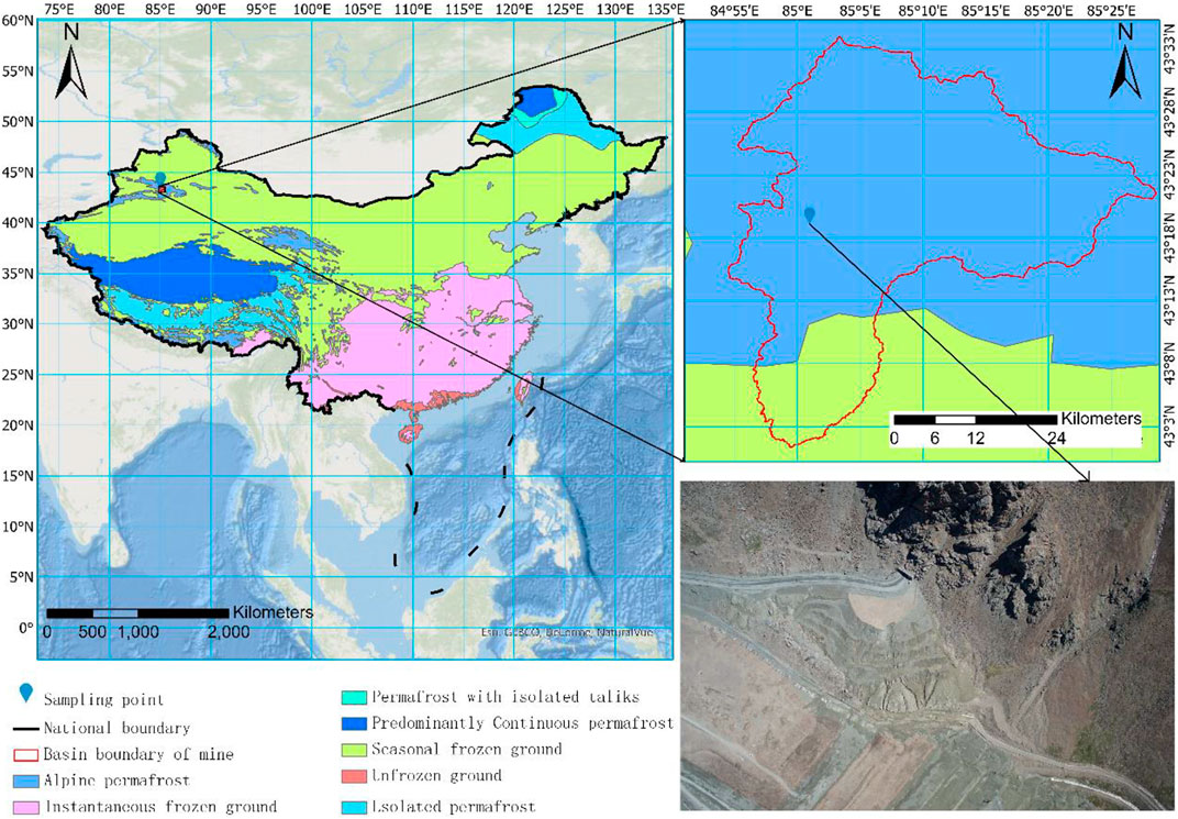
FIGURE 1. Schematic of the sampling location.

The mineral composition of the rock was determined using X-ray diffraction (XRD), and the results are shown in Figure 2. The fresh rock consisted of quartz (33.7%), albite and calcian (30.7%), microcline (25.1%), and other components (10.5%). Table 1 lists the chemical composition of the fresh rock, and then the rock was defined as granite.

FIGURE 2

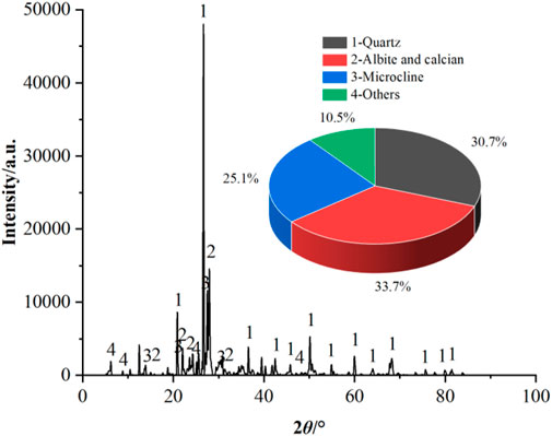
FIGURE 2. X-ray diffraction pattern.

TABLE 1

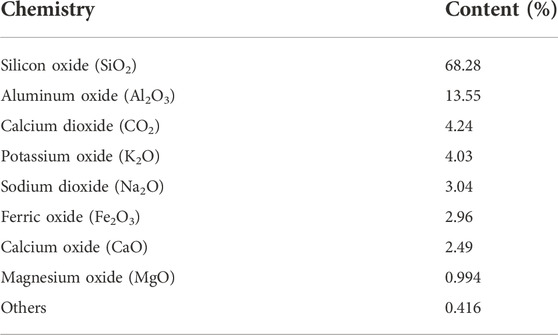
TABLE 1. Chemical composition of the tested rock.

The granite samples were obtained using the water drilling method. The samples were prepared according to international standards (ASTM, 2010) as cylinders with a diameter of 50 mm and height of 100 mm after cutting and grinding the rock block. The basic mechanical parameters of the tested rocks are presented in Table 2. To prevent ambiguity in the experimental tests, rock samples with evident defects were removed. Subsequently, rock samples with similar longitudinal wave velocities were selected for testing using a digital ultrasonic instrument to ensure the accuracy and reliability of the test results.

TABLE 2

TABLE 2. Basic mechanical parameters of the tested rock.

2.2 Test system

In this study, P-wave velocity tests, CT scanning, and uniaxial compression tests were performed on granite. The testing device as depicted in Figure 3.

1) F–T cycle test. The F–T cycle test was performed using an automatic concrete F–T testing device from China, which can display temperature change curves in real time and monitor the working state of the instrument. The measurement range of the F–T testing instrument was −25 to 25°C, and the accuracy was ±0.5°C. Temperature nonuniformity was within 2°C.

2) P–wave velocity test. The P-wave velocity of the rock under different numbers of F–T cycles was obtained using a digital ultrasonic instrument (RSM-SY5 (T)). The transmission pulse width of the instrument was continuously adjustable and ranged from 1 to 100 μs. The sampling interval was 0.1–200 μs, while the frequency bandwidth was between 300 and 500 kHz. The operating temperature ranged from −5 to 40°C. In this work, granite samples were subjected to P-wave velocity tests at room temperature (20°C) following varying numbers of F–T cycles.

3) CT test. A Philips Brilliance 16 spiral X-ray CT instrument, which was obtained from the State Key Laboratory of Frozen Soil Engineering (SKLFSE), Chinese Academy of Sciences (CAS), was used for scanning the granite samples after varying numbers of F–T cycles. The spatial resolution of the X-ray CT machine was 0.208 mm, the spatial resolution of the CT device was 24 lp/mm, and the density resolution was 0.3%. The scanning voltage, current, and layer thickness were determined by the density and porosity of the rock samples, and the scanning parameters were 120 kV, 313 mA, and 3 mm (Chen et al., 2019). In this study, CT scanning tests were conducted on up to 32 layers of granite samples at room temperature (20°C) after varying numbers of F–T cycles.

4) Uniaxial compression test. A GCTS RTR–1000 rock triaxial test system obtained from the SKLFSE, CAS, was employed to determine the mechanical characteristics of the granite. The test apparatus could withstand a maximum axial load of 1,000 kN, while the confining pressure ranged from 0 to 140 MPa. The pressure was resolved to within 0.01 MPa, and the accuracy of the deformation was ±2.0 mm (Zhang et al. 2022). The control temperature ranged from −30 to 80°C. In this study, uniaxial compression tests were conducted on granite samples at room temperature (20°C) at a loading rate of 0.5 MPa/s for different numbers of F–T cycles.

FIGURE 3

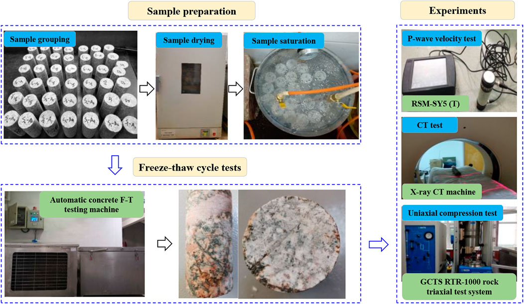
FIGURE 3. Test system and procedure.

2.3 Experiment procedure

As shown in Figure 3, the experimental steps are as follows:

1) Sample grouping. The prepared granite samples were sorted into six groups, each including three samples, depending on the variable numbers of F–T cycles. Five groups were used for mechanical tests after the F–T cycles, and the remaining group was used for CT scanning after the F–T cycles.

2) Sample drying. The selected samples were placed in a constant-temperature oven at 105°C for 48 h until the change in their mass did not exceed 0.1%. The samples were weighed after cooling to room temperature (20°C).

3) Sample saturation. The dry samples were saturated in distilled water under vacuum for 4 h, and then those were immersed in distilled water for more than 24 h to achieve sufficient water saturation.

4) Freeze–thaw procedure. The saturated sample was placed in an automatic concrete F–T testing machine, and the F–T tests were performed 0, 20, 40, 70, and 100 times. Based on actual measurements of environmental temperatures, the maximum and minimum air temperatures in the mining region were 13.1°C and –29.7°C, respectively (Zhou et al., 2022). Therefore, the freezing and thawing temperatures of the F–T cycle were set to –20 and 20°C, respectively, and the F–T cycle duration was approximately 6 h, as illustrated in Figure 4.

5) Experiments. After 0, 20, 40, 70, and 100 F–T cycles, the P-wave velocity test, CT scanning, and uniaxial compression tests of granite were conducted, respectively.

FIGURE 4

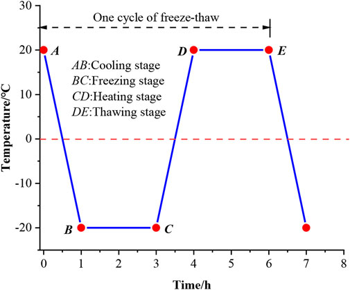
FIGURE 4. Temperature-time curve of F–T cycle.

2.4 Preparation of CT test

In this study, multilayer scanning was used for the CT scanning tests. To simplify the amount of data and facilitate comparative analysis, three scanning layers (scanning layers 2, 9, and 16) were selected from the 32 scanning layers for analysis, as shown in Figure 5A. Each layer was divided into three regions: S1 (marginal region), S2 (middle region), and S3 (central region), as shown in Figure 5B.

FIGURE 5

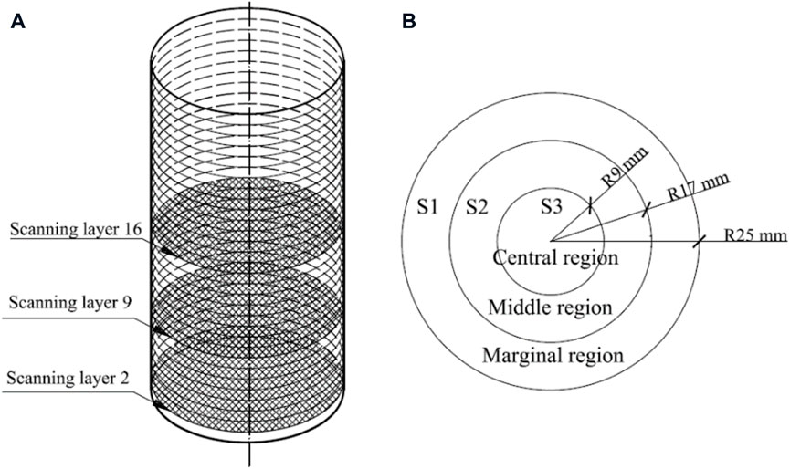
FIGURE 5. CT scanning layers. (A) scanning position; (B) regional division.

2.5 CT analysis principle

The standard equation for medical CT, which was established by Hounsfield in Britain in the 1970s (Hounsfield, 1973), is defined as

$H_{rm}=\frac{u_{rm}-u_{\omega }}{u_w}\times 1000,(1)$

where $H_{rm}$ is the CT value, $u_{rm}$ is the coefficient of X-ray absorption of the test sample, and $u_{\omega }$ is the coefficient of X-ray absorption of water.$u_{\omega }$ can be expressed as

$u_{rm}=u_m\rho ,(2)$

where $u_m$ is the absorption coefficient of a given substance, and ρ is its density.

Substituting Eq. 2 into Eq. 1, we obtain (Ketcham and Carlson, 2001; Zhang et al., 2019a, 2019b)

$\rho =\frac{{\mu }_{\omega }\left(1+\frac{H_{rm}}{1000}\right)}{u_m}.(3)$

If the scanning conditions and composition of the material do not change, the absorption coefficient of a particular substance $u_m$ is fixed, and equals 1, and we obtain

$u_m=\frac{1+\frac{H_{ro}}{1000}}{{\rho }_o},(4)$

where $H_{ro}$ is the CT value of the initial state of the material, and ${\rho }_o$ is the initial density of the material.

Eq. 5 is obtained by substituting Eq. 4 into Eq. 3

${\rho }_i=\frac{1+\frac{H_{ri}}{1000}}{\frac{1+\frac{H_{ro}}{1000}}{{\rho }_o}}={\rho }_o\times \frac{1000+H_{ri}}{1000+H_{ro}},(5)$

where ${\rho }_o$ is the initial density of the rock sample, ${\rho }_i$ is the density of the rock in the damaged state at time $i$, and $H_{ro}$ and $H_{ri}$ are the CT numbers of the rock in the states corresponding to ${\rho }_o$ and ${\rho }_i$, respectively.

3 Results and analyses

3.1 Mass and P-wave velocity under F–T cycles

The variations in the mass and P-wave velocity of granite subjected to different numbers of F–T cycles are illustrated in Figure 6. It can be seen from Figure 6, as the number of F–T cycles increases, the range of the increase in the granite mass is smaller (within 0.15 g). When the number of F–T cycles was 40 or higher, the mass of granite tended to remain constant. For instance, the mass of granite increased from 482.15 g to 482.3 g after 40 F–T cycles. This is caused by the fact that the water in the granite sample changed phases and generated a frost heaving force at negative temperatures, causing microcracks in the sample that increased the saturated water absorption of the granite sample and slightly improved the saturated mass of the sample (Park et al., 2015).

FIGURE 6

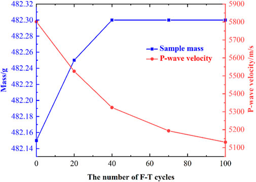
FIGURE 6. Mass and P-wave velocities of granite subjected to different numbers of F–T cycles.

Figure 6 shows the variation in the P-wave velocity of granite after different numbers of F–T cycles. The P-wave velocity of the granite samples showed a decreasing trend with an increase in the number of F–T cycles. After 0 to 40 F–T cycles, the P-wave velocity of the sample decreased significantly by 8.2%. During the period of 40–70 F–T cycles, the rate of decrease of the P-wave velocity of the sample decreased to 2.4%, and during the 70 to 100 F–T cycles, the P-wave velocity of the sample decreased by 1.2%. The attenuation of the P-wave velocity of granite with the number of F–T cycles reflects the F–T damage to the granite samples. Owing to the F–T cycles, original cracks and new damage cracks developed in the granite sample, and a large amount of water entered the sample to further accelerate the damage in the granite sample (Hori and Morihiro, 1998; Huang et al., 2020). Therefore, the P-wave velocity of the granite sample is decreased by moisture, microcracks, and pores.

3.2 Microstructural evolution properties of granite under F–T cycles

The microstructural evolution properties of granite were explored for various numbers of F–T cycles using an X-ray CT machine. The CT scanning test mainly reflects the damage expansion inside the rock mass based on changes in the CT values and CT images of different scanning layers. The evolution of the CT values of the entire sample was analyzed by calculating the mean (ME) and standard deviation (SD) of the CT values. The ME and SD values respectively reflect the variation and uniformity of rock density in the scanning layers. In this experiment, the saturated water contents of granite samples labeled No. 1 and No. 2 were 0.31% and 0.48%, respectively, which were used for CT scanning after different F–T cycles.

3.2.1 Damage evolution of granite under different numbers of F–T cycles

The ME and SD values for different scanned layers of granite under different numbers of F–T cycles are shown in Figures 7, 8, respectively, which reflect the rock damage after the F–T cycles. The naming convention for the samples is as follows. When “1-2” is taken as an example, “1” indicates sample No. 1 and “2” indicates the second scanning layer. Figure 7 indicates that the ME values of the second and ninth layers of granite decreased significantly after 20 F–T cycles, and then gradually increased until they became stable after 40 F–T cycles. After 20 F–T cycles, the ME values of samples No. 1 and No. 2 at the 16th layer located in the middle of the granite samples showed increasing and decreasing trends, respectively, and then gradually stabilized with a further increase in the number of F–T cycles. As illustrated in Figure 8, the SD values for granite sample No. 2 in different layers increased rapidly during the first 40 F–T cycles and then increased slowly with a subsequent increase in the number of F–T cycles. The SD values for granite sample No. 1 showed the same development trend as that of sample No. 2; however, the number of critical F–T cycles was 20. Because the saturated water content in sample No. 2 (0.48%) was higher than that in sample No. 1 (0.31%), the ME and SD values for granite sample No.2 varied more than those of sample No. 1 after the same number of F–T cycles. In other words, sample No. 2 suffered more severe F–T damage. From the evolution of the ME and SD values of granite samples under different F–T cycles, it can be inferred that the cycles caused new damage cracks in the granite samples, resulting in an uneven distribution of internal materials and reduced density (Park et al., 2015; Huang et al., 2022). Because of the low initial degree of damage of the granite samples, the F–T cycle had a greater impact on damage propagation in rock samples in the first 40 cycles of the F–T cycles than for larger numbers of F–T cycles under the action of water migration. However, with an increase in the number of F–T cycles, the overall damage in the granite samples continued to develop, and the degree of damage near the end of the sample was higher than that in the middle of the granite sample.

FIGURE 7

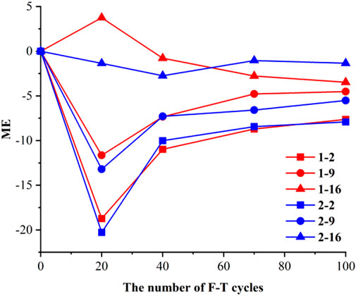
FIGURE 7. ME values for different scanning layers of granite under different numbers of F–T cycles.

FIGURE 8

FIGURE 8. SD values for different scanning layers of granite under different numbers of F–T cycles.

Figures 9, 10 show the variation curves of the ME and SD values of the granite samples in different regions (marginal region-S1, middle region-S2, and central region-S3) of the scanning layer with different numbers of F–T cycles. Because the ME and SD values for the second layer of the sample varied significantly, the second layer of the sample was selected as the scanning layer for analysis. The name of each sample was set according to the following convention. Considering “1-2-S1” as an example, “1” indicates sample No. 1, “2” indicates the second scanning layer, and “S1” indicates the scanning region (as shown in Figure 5B). After 20 F–T cycles, the ME values in S1 and S2 for the granite samples decreased. Subsequently, the densities of S1 and S2 increased after 40 F–T cycles, and the ME values increased slowly and gradually stabilized. As the number of F–T cycles increased, the F–T action prompted the granite sample to produce new damage cracks. Because of the water entering the cracks, the ME values increased in each region (S1, S2, and S3). The material distribution in the granite sample became uneven as a result of the generation of new cracks and the filling of water, which increased the SD value. A comparison of the different regions revealed that the change in ME and SD values in the marginal region (S1) is the largest, followed by the middle region (S2), and then the central region (S3). The decrease in ME values indicates that the density of the marginal and the middle region decreases to varying degrees, because of the formation of new damage cracks and the development of original microcracks caused by the cyclic F–T action. The slight increase in the ME value is the result of water entering the samples under the condition of minimal F–T damage.

FIGURE 9

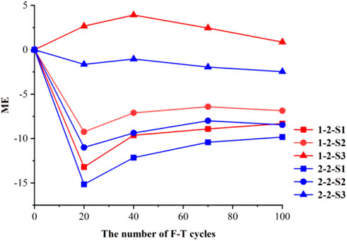
FIGURE 9. ME values for different regions of granite under different numbers of F–T cycles.

FIGURE 10

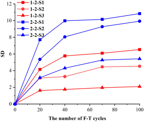
FIGURE 10. SD values for different regions of granite samples under different numbers of F–T cycles.

In view of the above analysis, the damage evolution of granite samples No. 1 and No. 2 is the same in different scanning regions for varying different numbers of F–T cycles; the damage of granite samples continued to develop with an increase in the number of F–T cycles; the damage of granite samples developed rapidly in the first 40 F–T cycles, and then gradually increased and eventually stabilized; the degree of damage of the marginal region of the sample was higher than that of other regions; and the degree of damage of sample No. 2 was higher than that of sample No. 1 owing to the higher saturated water content in sample No.2.

3.2.2 CT images of granite under different numbers of F–T cycles

CT images of the second, ninth, and sixteenth scanning layers of granite samples that underwent different numbers of F–T cycles are shown in Figures 11, 12, 13. The granite sample contained mineral particles, and its internal structure was uneven. In the image, lighter shades indicate higher-density regions, and darker shades indicate lower-density regions. The initial ME value of the granite sample was large, and the color brightness of the CT image was high. However, after 20 F–T cycles, the ME value of the granite test sample gradually decreased and the color of the CT image darkened. With an increase in the number of F–T cycles, new damage cracks were constantly generated in the granite samples, and more water entered the cracks, resulting in a continuous variation in the CT images of the granite samples. As indicated by the marks in Figure 11A, the location of the F–T damage was mainly concentrated in the marginal region of the granite sample. With an increase in the number of F–T cycles, the F–T damage regions gradually extended to the central regions.

FIGURE 11

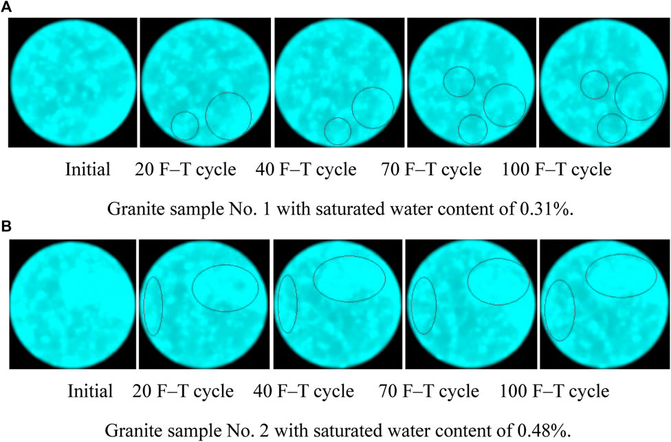
FIGURE 11. CT images of the second scanning layer for granite samples under different numbers of F–T cycles. Initial 20 F–T cycle 40 F–T cycle 70 F–T cycle 100 F–T cycle. (A) Granite sample No. 1 with saturated water content of 0.31%. Initial 20 F–T cycle 40 F–T cycle 70 F–T cycle 100 F–T cycle. (B) Granite sample No. 2 with saturated water content of 0.48%.

FIGURE 12

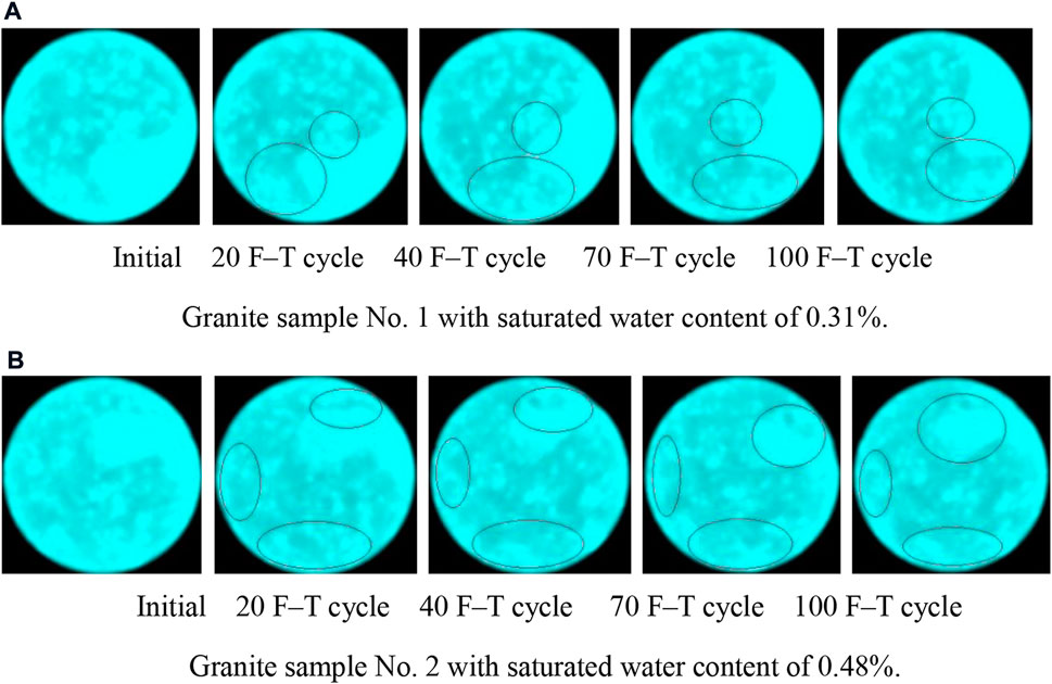
FIGURE 12. CT images of the ninth scanning layer for granite samples under different numbers of F–T cycles. Initial 20 F–T cycle 40 F–T cycle 70 F–T cycle 100 F–T cycle. (A) Granite sample No. 1 with saturated water content of 0.31%. Initial 20 F–T cycle 40 F–T cycle 70 F–T cycle 100 F–T cycle. (B) Granite sample No. 2 with saturated water content of 0.48%.

FIGURE 13

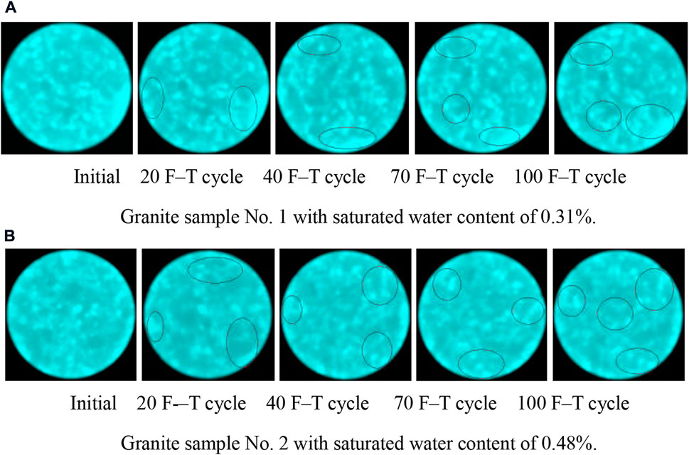
FIGURE 13. CT images of the 16th scanning layer for granite samples under different numbers of F–T cycles. Initial 20 F–T cycle 40 F–T cycle 70 F–T cycle 100 F–T cycle. (A) Granite sample No. 1 with saturated water content of 0.31%. Initial 20 F–T cycle 40 F–T cycle 70 F–T cycle 100 F–T cycle. (B) Granite sample No. 2 with saturated water content of 0.48%.

The following conclusions can be made from the CT values (ME and SD) and CT images of the granite samples shown in Figures 11–13. The F–T cycles promote the continuous development of initial microcracks and generate new damage cracks in granite, resulting in a decrease in the density of the sample and an uneven distribution of internal materials. With an increase in the number of F–T cycles, the ME value decreased while the SD value increased, and the damage location gradually shifted towards the central region of the granite sample. The ends and marginal regions of the granite samples were easily damaged, and the degree of damage was higher than that in the other regions. The saturated water content and initial damage state of the granite samples played an important role in the aggravation of damage.

3.3 Macroscopic mechanical properties of granite under F–T cycles

The axial stress-strain curves of granite after undergoing different numbers of F–T cycles are shown in Figure 14. It can be observed that the shapes of the stress strain curves of the granite sample under different F-T cycle are similar. After achieving their peak stress, the granite samples rapidly disintegrated, and the stress-strain curves decreased rapidly. Based on the overall characteristics of the stress-strain curves of the granite sample, the curves can be divided into the following stages: compaction deformation, elastic deformation, plastic yield, and strain softening (Gao et al., 2020). During the compaction deformation stage, the initial microcracks of the granite gradually closed, and the granite sample was compacted. With continuous loading, the granite sample gradually entered the elastic deformation stage, and the strain increased linearly with an increase in stress. When the stress reached the yield limit, the granite sample entered the plastic yield stage. Subsequently, the strain of the sample increased nonlinearly with an increase in stress, resulting in irreversible deformation. When the stress reached the ultimate strength, the granite sample reached the strain softening stage; the crack in the sample developed rapidly, and the strength decreased rapidly. Finally, the granite sample was destroyed (Zhang et al., 2020). Meanwhile, different numbers of F–T cycles led to different characteristics of the stress-strain curves at each stage. The compaction deformation stage and elastic deformation stage grew linearly with an increase in stress, and the stress-strain curves under different F–T cycles were not easily distinguishable. As the number of F–T cycles increased, the plastic yield gradually decreased.

FIGURE 14

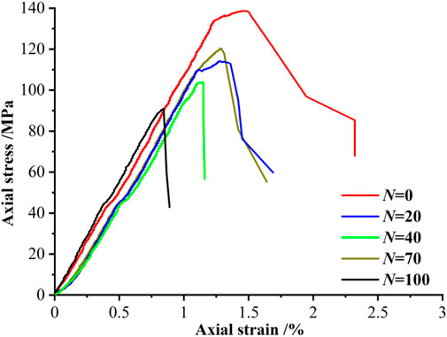
FIGURE 14. Axial stress-strain curves for granite under different numbers of F–T cycles.

Based on Figure 14 and Table 3 presents the uniaxial test results for the granite sample under different numbers of F–T cycles. It can be observed that with an increase in the number of F–T cycles, the peak strength (${\sigma }_t$), elastic modulus ($E$), and coefficient of frost resistivity (K_f = R₁/R₂, where R₁ and R₂ are respectively the uniaxial compressive strengths of the saturated rock before and after the F–T cycles) gradually decreased.

TABLE 3

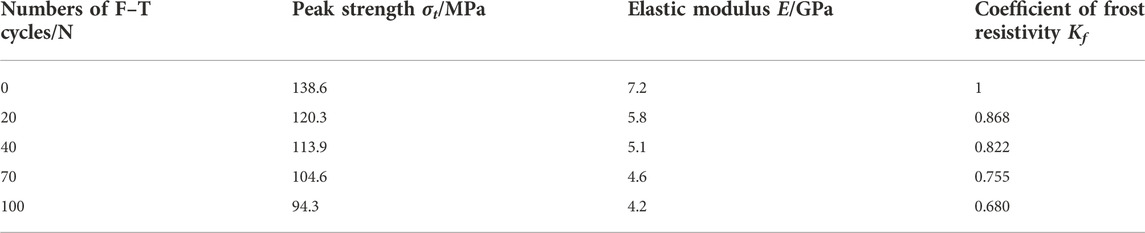
TABLE 3. Uniaxial test results for granite.

Figures 15, 16 present the variation curves of the peak strength, elastic modulus, and coefficient of frost resistivity of granite for different numbers of F–T cycles. The macroscopic mechanical properties of granite under different F–T cycles are shown as follows: 1) the peak strength of granite samples without the F–T cycle was 138.6 MPa, and the loss rates of compressive strength after 20, 40, 70, and 100 F–T cycles were 13.2%, 18.8%, 24.5%, and 39.1% respectively, indicating that the F–T action has a significant impact on the mechanical properties of granite; 2) the elastic modulus of the granite samples decreased significantly after the F–T cycles, and the F–T cycles aggravated the damage to granite. Before the F–T cycles, the elastic modulus was 7.2 GPa, and after the first 20 F–T cycles, it was 5.8 GPa, corresponding a decrease of 19.4%. After 100 F-T cycles, the elastic modulus was 4.2 GPa, which is a decrease of 41.6%; 3) the coefficient of frost resistivity refers to the resistance of rocks to F–T damage. With an increase in the number of F–T cycles, the coefficient of frost resistivity of granite gradually decreased.

FIGURE 15

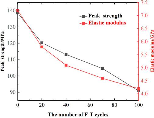
FIGURE 15. Peak strength and elastic modulus of granite under different numbers of F–T cycles.

FIGURE 16

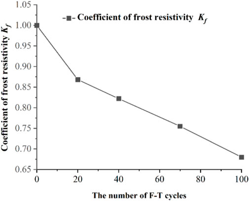
FIGURE 16. Coefficient of frost resistivity of granite under different numbers of F–T cycles.

It is clear from the text above that as the number of F–T cycles increases, the macroscopic mechanical characteristics of granite rapidly deteriorate. The granite sample’s slightly weathered structure during the first freezing and thawing processes is what creates this phenomenon, which results in considerable damage from the F–T action. However, owing to granite is a dense and hard rock with low saturated water content, the damage caused by F–T cycles to the unweathered compact structure inside the rock sample is gradual. Meanwhile, with an increase in the number of F–T cycles, the degree of damage of the granite sample increased, resulting in a gradual decrease in the elastic modulus. However, with a further increase in the number of F–T cycles, there was less damage to granite due to the F–T cycle. The results reveal that the F–T action can cause irreversible damage to granite. The granite damage is evident at the initial stage of the F–T cycle, and the degree of damage due to the F–T cycle gradually decreases.

3.4 Damage evolution equation of granite under F–T cycles

The F–T weathering of rocks is a long-term process. The F–T cycles not only deteriorate the macroscopic mechanical properties, such as the mechanical strength and elastic modulus of the rock, but also deteriorated the microscopic structure of the rock. The macro-microscopic damage evolution equation of rock under cyclic F–T action was deduced based on the mechanical and microstructural parameters of granite after F–T cycles.

Micropores and joint fissures are also present in natural rocks. During the F–T cycles, the frost heaving force caused by the phase transformation of water freezing in the fissures gradually expands the cracks, resulting in a decrease in rock strength. In previous studies, micropores and joint fissures in rocks have been defined as the initial damage to the rock material. However, because of the complexity of the rock structures, as inferred from the variations in their sizes, shapes, and bonding modes of mineral particles, it is difficult to determine the damage variable of a rock’s intact state. Therefore, the damage variable in the initial state can be used to replace the damage variable in the intact state, and the degree of change in the damage can also be described by the damage variable. The damage variables were defined as follows (Chen et al., 2019):

$D=\{\begin{array}{cc}0& \begin{array}{cccc}Condition& of& no& damage\end{array}\\ 0<D<1& \begin{array}{cccc}State& of& damage& evolution\end{array}\\ 1& \begin{array}{cccc}State& of& complete& failure\end{array}\end{array}(6)$

3.4.1 Defining damage variables using elastic modulus

The variation in the elastic modulus of the rock represents the degree of internal damage to the material. Therefore, the F–T damage evolution equation of the rock can be expressed as:

$D_E=1-\frac{E_n}{E_o},(7)$

where $D_E$ is the F–T damage value, $E_o$ is the initial elastic modulus of the rock before F–T cycles, and $E_n$ is the elastic modulus of the rock after n F–T cycles.

3.4.2 Defining damage variables using density

The F–T cycles can cause changes in the densities of the rock samples. The damage variable can be determined based on the relative difference between the damaged state densities (Lemaitre and Dufailly, 1987).

$D_{\rho }={\left(1-\frac{{\rho }_i}{{\rho }_o}\right)}^{2/3},(8)$

where ${\rho }_o$ is the initial density of the rock, and ${\rho }_i$ is the density of the rock under the damaged state at time i.

By combining Eqs 3, 8, the following can be obtained.

$D{}_{\rho }={\left(1-\frac{{\mathit{\mu }}_{\omega }\left(1+\frac{H_{ri}}{1000}\right)}{u_{mi}}\times \frac{u_{mo}}{{\mathit{\mu }}_{\omega }\left(1+\frac{H_{ro}}{1000}\right)}\right)}^{2/3},(9)$

where ${\mu }_{m\mathit{0}}$ and ${\mu }_{mi}$ are the absorption coefficients of the substance at different times.

Because the material composition of the rock sample remained unchanged during the freezing and thawing processes,

$u_{mi}=u_{mo}(10)$

Then, Eq. 9 can be simplified to Eq. 11 as

$D_{\rho }={\left(\frac{H_{ro}-H_{ri}}{1000+H_{ro}}\right)}^{2/3}.(11)$

Considering the influence of the instrument resolution, the rock damage variable is as follows:

$D_{\rho }=\frac{1}{m_o}{\left(\frac{H_{ro}-H_{ri}}{1000+H_{ro}}\right)}^{2/3},(12)$

where $m_o$ is the spatial resolution of CT scanning, $H_{ro}$ is the CT value of the initial state of the rock material, and $H_{ri}$ is the CT value of the rock material after the F–T cycle.

3.4.3 Defining damage variables using porosity

If the porosity changes of the rock after F–T cycles is $∆n$, then

$\Delta n=n_{ri}-n_{ro},(13)$

where $n_{ri}$ is the porosity of the rock after i F–T cycles, and $n_{ro}$ is the porosity of the rock in its initial state before the F–T cycles.

According to the porosity changes of granite samples after a certain number of F–T cycles in Table 4, the relationship between the porosity changes and elastic modulus of granite samples after a certain number of F–T cycles was analyzed, as shown in Figure 17. And Eq. 14 was obtained by fitting. The elastic modulus of granite increased linearly with increasing porosity during the F–T cycles.

$E_n=E_o-a\cdot \mathrm{\Delta }n,(14)$

where $∆n$ is the change in porosity of granite after an F–T cycle, and a is the slope parameter.

TABLE 4

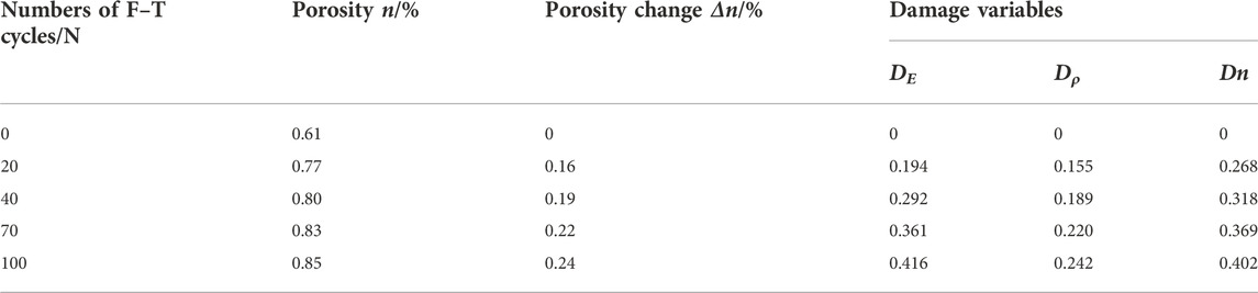
TABLE 4. Porosity change and damage variables of granite samples for different F–T cycles.

FIGURE 17

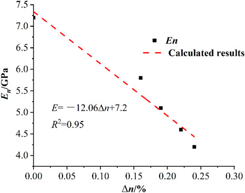
FIGURE 17. Relationship between the elastic modulus and porosity change of the granite sample.

The damage variable defined by the elastic modulus is shown in Eq. 7. By combining Eqs 7, 14, the following can be obtained:

$D_n=\frac{a}{E_o}\mathrm{\Delta }n,(15)$

According to the test results of granite samples for different F–T cycles in this study, as shown in Figure 17, E_o = 7.2 and a = 12.06. Therefore, we can obtain Eq. 16 and the values in Table 4.

$D_n=1.675·\mathrm{\Delta }n.(16)$

Eqs 7, 12, 16 characterize the decay process of the internal microstructure of the rocks under F–T cycles, and they reflect the degree of damage to the rocks. According to the microstructural parameters of the selected granite samples after different numbers of F–T cycles, the damage variables of the granite samples for the corresponding numbers of F–T cycles in Table 4 can be obtained from three equations. The damage variables and F–T cycle times are shown in Figure 18. The following features can be clearly identified: 1) the damage variables defined by different parameters can accurately characterize the degree of damage to granite under F–T cycles; 2) the damage variables of granite increase continuously as the number of F–T cycles increases; and 3) the damage variables increase rapidly when the number of F–T cycles is less than 40, and gradually decrease for the number of F–T cycles greater than 40.

FIGURE 18

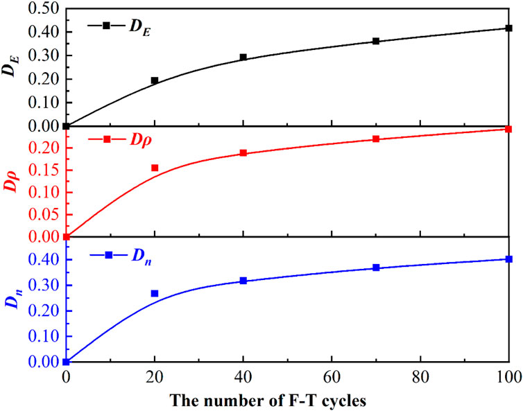
FIGURE 18. Relationship between F–T damage variables and number of F–T cycles.

4 Conclusion

In this study, several experimental tests in which granite was subjected to 0, 20, 40, 70, and 100 F–T cycles using a uniaxial compression apparatus and CT technology were performed. The evolution of the mechanical behavior and damage to granite was analyzed under the F–T cycles. The conclusions drawn from this study are summarized as follows.

1) As the number of F–T cycles increased, the mass of granite changed slightly (within 0.15 g), and the P-wave velocity, peak strength, elastic modulus, and coefficient of frost resistivity of the granite gradually decreased. After 0 to 40 F–T cycles, the P-wave velocity, peak strength, and elastic modulus of the granite sample decreased by 8.2%, 18.8%, and 29.1%, respectively. The degree of the F–T damage in rocks is influenced by the saturated water content and the initial damage state.

2) The F–T cycle significantly influenced the damage extension in the early stage, but there was little influence in the later stage. Under different numbers of F–T cycles (0–100 times) in this study, variations in the damage variables of granite with an increase in the number of F–T cycles can be divided into two phases. In the first phase (< 40 F–T cycles), the damage variable of granite increased rapidly, and the damage variable of granite gradually stabilized after 40 F–T cycles in the second phase.

3) Based on the characteristics of the CT results, with an increase in the number of F–T cycles, the damage gradually extended to the central region of the granite sample. The ends and marginal regions of the granite samples were easily damaged, and the degree of damage was higher than that in the other regions.

4) Three damage variables with different definitions (elastic modulus, density, and porosity) can accurately characterize the degree of damage to granite under the F–T cycle.

Data availability statement

The original contributions presented in the study are included in the article/supplementary material, further inquiries can be directed to the corresponding author.

Author contributions

DC: Roles/Writing—original draft, Data curation, Formal analysis, Resources, Methodology. GL: Funding acquisition, Writing—review and editing, Supervision. JL: Resources. QD: Visualization. All other co-authors reviewed and supervised the manuscript, and all listed authors approved it for publication.

Funding

This study was supported by the China’s Second Tibetan Plateau Scientific Expedition and Research (2019QZKK0905), the National Natural Science Foundation of China (No. 42201162), the State Key Laboratory for Geomechanics and Deep Underground Engineering, the China University of Mining and Technology (SKLGDUEK1904), and the Research Project of the State Key Laboratory of Frozen Soils Engineering (Grant No. SKLFSE-ZY-20, SKLFSE-ZQ-58, SKLFSE-ZT-202203).

Conflict of interest

The authors declare that the research was conducted in the absence of any commercial or financial relationships that could be construed as a potential conflict of interest.

Publisher’s note

All claims expressed in this article are solely those of the authors and do not necessarily represent those of their affiliated organizations, or those of the publisher, the editors and the reviewers. Any product that may be evaluated in this article, or claim that may be made by its manufacturer, is not guaranteed or endorsed by the publisher.

References

ASTM D7012-10 (2010). Standard test methods for compressive strength and elastic moduli of intact rock core specimens under varying states of stress and temperatures. ASTM Int. 2010, 06. doi:10.1520/D7012-10

CrossRef Full Text | Google Scholar

Bayram, F. (2012). Predicting mechanical strength loss of natural stones after freeze–thaw in cold regions. Cold Reg. Sci. Technol. 83-84, 98–102. doi:10.1016/j.coldregions.2012.07.003

CrossRef Full Text | Google Scholar

Chang, Z., Cai, Q., Li, M., and Han, L. (2018). Sensitivity analysis of factors affecting time dependent slope stability under freeze-thaw cycles. Math. Probl. Eng. 2018, 1–10. doi:10.1155/2018/7431465

CrossRef Full Text | Google Scholar

Chen, T. C., Yeung, M. R., and Mori, N. (2004). Effect of water saturation on deterioration of welded tuff due to freeze-thaw action. Cold Reg. Sci. Technol. 38 (2-3), 127–136. doi:10.1016/j.coldregions.2003.10.001

CrossRef Full Text | Google Scholar

Chen, S., Ma, W., and Li, G. (2019). Study on the mesostructural evolution mechanism of compacted loess subjected to various weathering actions. Cold Reg. Sci. Technol. 167, 102846. doi:10.1016/j.coldregions.2019.102846

CrossRef Full Text | Google Scholar

Fan, L. F., Xu, C., and Wu, Z. J. (2020). Effects of cyclic freezing and thawing on the mechanical behavior of dried and saturated sandstone. Bull. Eng. Geol. Environ. 79 (2), 755–765. doi:10.1007/s10064-019-01586-z

CrossRef Full Text | Google Scholar

Gao, F., Cao, S., Zhou, K., Lin, Y., and Zhu, L. (2020). Damage characteristics and energy-dissipation mechanism of frozen-thawed sandstone subjected to loading. Cold Reg. Sci. Technol. 169, 102920. doi:10.1016/j.coldregions.2019.102920

CrossRef Full Text | Google Scholar

Ghobadi, M. H., and Babazadeh, R. (2015). Experimental studies on the effects of cyclic freezing–thawing, salt crystallization, and thermal shock on the physical and mechanical characteristics of selected sandstones. Rock Mech. Rock Eng. 48 (3), 1001–1016. doi:10.1007/s00603-014-0609-6

CrossRef Full Text | Google Scholar

Hori, M., and Morihiro, H. (1998). Micromechanical analysis on deterioration due to freezing and thawing in porous brittle materials. Int. J. Eng. Sci. 36 (4), 511–522. doi:10.1016/S0020-7225(97)00080-3

CrossRef Full Text | Google Scholar

Hounsfield, G. N. (1973). Computerized transverse axial scanning (tomography): Part 1. Description of system. Br. J. Radiol. 46 (552), 1016–1022. doi:10.1259/0007-1285-46-552-1016

PubMed Abstract | CrossRef Full Text | Google Scholar

Huang, S., Liu, Y., Guo, Y., Zhang, Z., and Cai, Y. (2019). Strength and failure characteristics of rock-like material containing single crack under freeze-thaw and uniaxial compression. Cold Reg. Sci. Technol. 162, 1–10. doi:10.1016/j.coldregions.2019.03.013

CrossRef Full Text | Google Scholar

Huang, S., Lu, Z., Ye, Z., and Xin, Z. (2020). An elastoplastic model of frost deformation for the porous rock under freeze-thaw. Eng. Geol. 278, 105820. doi:10.1016/j.enggeo.2020.105820

CrossRef Full Text | Google Scholar

Huang, S., Cai, C., Yu, S. L., He, Y. B., and Cui, X. Z. (2022). Study on damage evaluation indexes and evolution models of rocks under freeze-thaw considering the effect of water saturations. Int. J. Damage Mech. 6 (0), 105678952211062–29. doi:10.1177/10567895221106241

CrossRef Full Text | Google Scholar

Jamshidi, A., Nikudel, M. R., and Khamehchiyan, M. (2013). Predicting the long-term durability of building stones against freeze–thaw using a decay function model. Cold Reg. Sci. Technol. 92, 29–36. doi:10.1016/j.coldregions.2013.03.007

CrossRef Full Text | Google Scholar

Jia, H., Ding, S., Zi, F., Dong, Y., and Shen, Y. (2020). Evolution in sandstone pore structures with freeze-thaw cycling and interpretation of damage mechanisms in saturated porous rocks. Catena 195, 104915. doi:10.1016/j.catena.2020.104915

CrossRef Full Text | Google Scholar

Ketcham, R. A., and Carlson, W. D. (2001). Acquisition, optimization and interpretation of X-ray computed tomographic imagery: Applications to the geosciences. Comput. Geosci. 27 (4), 381–400. doi:10.1016/s0098-3004(00)00116-3

CrossRef Full Text | Google Scholar

Lemaitre, J., and Dufailly, J. (1987). Damage measurements. Eng. Fract. Mech. 28 (5–6), 643–661. doi:10.1016/0013-7944(87)90059-2

CrossRef Full Text | Google Scholar

Li, S. Y., Lai, Y. M., Pei, W. S., Zhang, S., and Zhong, H. (2014). Moisture-temperature changes and freeze-thaw hazards on a canal in seasonally frozen regions. Nat. Hazards 72 (2), 287–308. doi:10.1007/s11069-013-1021-3

CrossRef Full Text | Google Scholar

Liu, Q., Huang, S., Kang, Y., and Liu, X. (2015). A prediction model for uniaxial compressive strength of deteriorated rocks due to freeze–thaw. Cold Reg. Sci. Technol. 120, 96–107. doi:10.1016/j.coldregions.2015.09.013

CrossRef Full Text | Google Scholar

Liu, L., Qin, S. N., and Wang, X. C. (2018). Poro-elastic–plastic model for cement-based materials subjected to freeze–thaw cycles. Constr. Build. Mat. 184, 87–99. doi:10.1016/j.conbuildmat.2018.06.197

CrossRef Full Text | Google Scholar

Liu, T., Zhang, C., Cao, P., and Zhou, K. (2020). Freeze-thaw damage evolution of fractured rock mass using nuclear magnetic resonance technology. Cold Reg. Sci. Technol. 170, 102951. doi:10.1016/j.coldregions.2019.102951

CrossRef Full Text | Google Scholar

Lu, Y., Li, X., and Chan, A. (2019). Damage constitutive model of single flaw sandstone under freeze-thaw and load. Cold Reg. Sci. Technol. 159, 20–28. doi:10.1016/j.coldregions.2018.11.017

CrossRef Full Text | Google Scholar

Martínez-Martínez, J., Benavente, D., Gomez-Heras, M., Marco-Castaño, L., and Ángeles Garcíadel- Cura, M. (2013). Non-linear decay of building stones during freeze–thaw weathering processes. Constr. Build. Mat. 38, 443–454. doi:10.1016/j.conbuildmat.2012.07.059

CrossRef Full Text | Google Scholar

Momeni, A., Abdilor, Y., Khanlari, G., Heidari, M., and Sepahi, A. (2016). The effect of freeze-thaw cycles on physical and mechanical properties of granitoid hard rocks. Bull. Eng. Geol. Environ. 75 (4), 1649–1656. doi:10.1007/s10064-015-0787-9

CrossRef Full Text | Google Scholar

Mu, J. Q., Pei, X. J., Huang, R. Q., Rengers, N., and Zou, X. q. (2017). Degradation characteristics of shear strength of joints in three rock types due to cyclic freezing and thawing. Cold Reg. Sci. Technol. 138, 91–97. doi:10.1016/j.coldregions.2017.03.011

CrossRef Full Text | Google Scholar

Mutlutürk, M., Altindag, R., and Türk, G. (2004). A decay function model for the integrity loss of rock when subjected to recurrent cycles of freezing-thawing and heating-cooling. Int. J. Rock Mech. Min. Sci. (1997). 41 (2), 237–244. doi:10.1016/S1365-1609(03)00095-9

CrossRef Full Text | Google Scholar

Nicholson, H., Dawn, T., and Nicholson, F. H. (2000). Physical deterioration of sedimentary rocks subjected to experimental freeze-thaw weathering. Earth Surf. Process. Landf. 25 (12), 1295–1307. doi:10.1002/1096-9837(200011)25:12<1295::AID-ESP138>3.0.CO;2-E

CrossRef Full Text | Google Scholar

Park, J., Hyun, C. U., and Park, H. D. (2015). Changes in microstructure and physical properties of rocks caused by artificial freeze-thaw action. Bull. Eng. Geol. Environ. 74 (2), 555–565. doi:10.1007/s10064-014-0630-8

CrossRef Full Text | Google Scholar

Remy, J. M., Bellanger, M., and Homand-Etienne, F. (1994). Laboratory velocities and attenuation of P-waves in limestones during freeze–thaw cycles. Geophysics 59 (2), 245–251. doi:10.1190/1.1443586

CrossRef Full Text | Google Scholar

Shen, Y. J., Yang, G. S., Huang, H. W., Rong, T. L., and Jia, H. L. (2018). The impact of environmental temperature change on the interior temperature of quasi-sandstone in cold region: Experiment and numerical simulation. Eng. Geol. 239, 241–253. doi:10.1016/j.enggeo.2018.03.033

CrossRef Full Text | Google Scholar

Sun, Y., Zhai, C., Xu, J., Cong, Y., Qin, L., and Zhao, C. (2020). Characterisation and evolution of the full size range of pores and fractures in rocks under freeze-thaw conditions using nuclear magnetic resonance and three-dimensional X-ray microscopy. Eng. Geol. 271, 105616. doi:10.1016/j.enggeo.2020.105616

CrossRef Full Text | Google Scholar

Yang, G., Xie, D., and Zhang, C. (1998). The quantitative analysis of distribution regulation of CT values of rock damage. Chin. J. Rock Mech. Eng. 17 (3), 279–285.

Google Scholar

Zhang, G., Liu, E., Chen, S., and Zhang, D. (2019a). Damage constitutive model based on energy dissipation for frozen sandstone under triaxial compression revealed by X-ray tomography. Exp. Tech. 43 (5), 545–560. doi:10.1007/s40799-019-00309-z

CrossRef Full Text | Google Scholar

Zhang, G., Liu, E., Chen, S., and Song, B. (2019b). Micromechanical analysis of frozen silty clay-sand mixtures with different sand contents by triaxial compression testing combined with real-time CT scanning. Cold Reg. Sci. Technol. 168 (12), 102872. doi:10.1016/j.coldregions.2019.102872

CrossRef Full Text | Google Scholar

Zhang, H., Meng, X., and Yang, G. (2020). A study on mechanical properties and damage model of rock subjected to freeze-thaw cycles and confining pressure. Cold Reg. Sci. Technol. 174, 103056. doi:10.1016/j.coldregions.2020.103056

CrossRef Full Text | Google Scholar

Zhang, L., Niu, F. J., Liu, M. H., Luo, J., and Ju, X. (2022). Mechanical behavior of cracked rock in cold region subjected to step cyclic loading. Geofluids 2022, 1–15. doi:10.1155/2022/6220549

CrossRef Full Text | Google Scholar

Zhou, Y., Li, G. Y., Jin, H. J., Marchenko, S. S., Ma, W., Du, Q. S., et al. (2022). Viscous creep of ice-rich permafrost debris in A recently uncovered proglacial area in the tianshan mountains, China. Adv. Clim. Change Res. 2022, 540–553. doi:10.1016/j.accre.2022.05.005

CrossRef Full Text | Google Scholar