Deep-learning-based surrogate model for fast and accurate simulation in pipeline transport

A new deep-learning-based surrogate model is developed and applied for predicting dynamic temperature, pressure, gas rate, oil rate, and water rate with different boundary conditions in pipeline flow. The surrogate model is based on the multilayer perceptron (MLP), batch normalization and Parametric Rectified Linear Unit techniques. In training, the loss function for data mismatch is considered to optimize the model parameters with means absolute error (MAE). In addition, we also use the dynamic weights, calculated by the input data value, to increase the contribution of smaller inputs and avoid errors caused by large values eating small values in total loss. Finally, the surrogate model is applied to simulate a complex pipeline flow in the eastern part of the South China Sea. We use flow and pressure boundary as the input data in the numerical experiment. A total of 215690 high-fidelity training simulations are performed in the offline stage with commercial software LeadFlow, in which 172552 simulation runs are used for training the surrogate model, which takes about 240 min on an RTX2060 graphics processing unit. Then the trained model is used to provide pipeline flow forecasts under various boundary conduction. As a result, it is consistent with those obtained from the high-fidelity simulations (e.g., the media of relative error for temperature is 0.56%, pressure is 0.79%, the gas rate is 1.02%, and oil rate is 1.85%, and water is 0.80%, respectively). The online computations from our surrogate model, about 0.008 s per run, achieve speedups of over 1,250 relative to the high-fidelity simulations, about 10 s per run. Overall, this model provides reliable and fast predictions of the dynamic flow along the pipeline.

1 Introduction

Pipe network simulation has essential research value in oil and gas production. In the realistic gas pipeline on the sea, the gas-liquid two-phase flow and the terrain both are complex and variable; any change in the environment will directly affect the normal operation of the gathering transportation network. On the other hand, the long oil and gas gathering pipeline will cause significant instability in transportation. All these will complicate the pipeline’s simulation calculation and operation management.

Due to the complexity of the gas-liquid two-phase flow, it is not easy to accurately simulate the distribution law along the submarine oil-gas mixed transportation pipeline. Countries worldwide have invested a lot of human and material resources to study the calculation of oil-gas mixed transportation pipeline networks and formed commercial simulation software, including PipePhase, PipeSIM, PETITE, OLGA, and LedaFlow. The reference (Xie et al., 2022) established a wax deposition model in a submarine pipeline using the OLGA wax deposition module. Using this model, they analyzed the influence of five factors on oil-gas-water three-phase wax deposition: oil flow rate, water content, inlet temperature, gas-oil ratio, and outlet pressure. Because the cost is expensive for commercial software, many researchers have also explored pipeline flow problems using numerical experimental methods. The reference (AUNICKY 1970) proposed and tested the new empirical correlations, including the influence of the flow length on the growth of the dispersion coefficient’s value and the influence of the Reynolds’ number and concentration boundary upon the final volume. They pointed out that a Taylor-type model is not entirely satisfactory since the dispersion coefficient seems to increase with the length of the pipe and not stay constant. The reference (Rachid et al., 2002) presented a model for predicting the contaminated mixing volume arising in pipeline batch transfers without physical separators. They considered the time-dependent flow rates and accurate concentration-varying axial dispersion coefficients. In addition to this, they coupled the finite element method and Newton’s method to solve the governing equation. In this way, they exhibited the best estimate over the whole range of admissible concentrations investigated. The reference (Al-Sarkhi and Hanratty., 2002) used a laser diffraction technique to measure the drop size distributions for air and water flowing in an annular pattern in a 2.54 cm horizontal pipe. The reference (de Freitas Rachid et al., 2002) proposed a new model for estimating mixing volumes arising in batch transfers in multiproduct pipelines when variations of the line diameter and injection and withdrawal of products are present. The reference (Lain and Sommerfeld. 2012) studied the problem of pneumatic conveying for spherical particles in horizontal ducts, a 6 m long rectangular cross-section horizontal channel, and a circular pipe. They calculated the three-dimensional numerical by the Euler–Lagrange approach in connection with the k–ε and a Reynolds Stress turbulence model accounting for full two-way coupling. In the reference (Kang et al., 2014), the mechanism of factors affecting wax deposition, which are related to mitigation technologies, was presented. The reference (Aman et al., 2016) used a single-pass, gas-dominant flow loop to study the effect of gas velocity on hydrate formation and deposition rate in the pipeline. In the reference (Xiong et al., 2022), the opposition-based learning strategy and the adaptive T-distribution mutation operator were introduced to overcome the DELM effect’s effect on the random input weight in each ELM-AE and improve the quantitative prediction performance. The reference (Marfatia and Li. 2022) simplified the commonly used model in the FCMP. It was extended to address a pipeline network, for which the mixing effect at the pipeline junctions is addressed. However, due to the complexity of the pipe network simulation calculation, neither software nor numerical methods can quickly simulate the whole pipeline system in real-time. At the same time, considering the oil and gas reservoir uncertainty, the development process often needs many simulations of the whole pipeline network under different production conditions. So, it is challenging to meet the demand for the pipeline network’s traditional simulation-based steady/unsteady flow calculation method. Therefore, how to build fast surrogate models has become the focus of many researchers.

With the rapid development of deep learning in image and natural language processing, more and more researchers are constructing corresponding reservoir surrogate models based on deep learning techniques. The reference (Wang et al., 2018) used the long and short-term memory (Gers et al., 2000) networks to approximate the flow dynamics model in a low-dimensional subspace constructed by POD. The reference (Bruyelle and Guerillot, 2019) applied the network architecture based on image processing to geological modeling. The proposed approach provided accurate prediction results to speed up and improve the history matching process. The reference (Tang et al., 2020) introduced a proxy model R-U-NET based on deep learning to predict the flow response of different geological models. They could quickly and accurately simulate reservoir changes and be used to solve history matching problems. The reference (Zhou et al., 2022) proposed a novel dynamic simulation method based on an interpretable shortcut Elman network (Shortcut-ENN) model for the pipeline network. The Shortcut-ENN model is derived from the state-space equations. Based on the Shortcut-ENN model, the pipeline’s connection relationship and mechanism characteristics are retained. The reference (Spandonidis et al., 2022) constructed a 2D-Convolutional Neural Network model that undertakes supervised classification in spectrograms extracted by the accelerometers’ signals on the pipeline wall. Then, the model was used to immediately detect leaks in metallic piping systems to transport liquid and gaseous petroleum products.

Because we have fast and accurate reservoir simulation based on machine learning, we consider using the deep-learning model to simulate the pipeline change in oil or gas transport. In this paper, we reduce the work of pipeline simulation to a regression problem and use multiplayer perceptron (MLP) based on full connected (FC) to construct our surrogate model. We propose three key improvements in our model. Firstly, the FC + PReLU + BN structure is used to construct the surrogate model; this proves that deep learning can be used in pipeline simulation. Then PReLU is used to solve the problem of neuronal necrosis caused by ReLU in the activation operation. Finally, the weights of the loss function are dynamically decided by the value of the input.

The content of this paper proceeds as follows: In the second section, we give the detail of the surrogate model proposed in this paper. We introduce the structure of the surrogate model, the loss functions, and the data preprocessing process. In the third section, we use a realistic gas pipeline on the sea to illustrate the performance of our surrogate model. Finally, the conclusions are summarized, and future work is discussed.

2 Principle of model framework

In the pipeline, we use the flow boundary of every well and the pressure boundary at the endpoint as the input data. The flow boundary contains gas flow rate, oil flow rate, water flow rate, and temperature. The pressure boundary is mainly the pressure at the endpoint of the pipeline. In this paper, we mainly use the surrogate model to get the change in gas flow rates, oil flow rates, water flow rates, pressures, and temperatures at each point along the pipeline. Therefore, the process can be reduced to a regression network model. At the same time, since a one-dimensional structure is often used to represent pipelines, we use an MLP as the basis to construct the surrogate model. In this part, we will introduce some detailed information about MLP, then the overall model architecture will be described, and finally, the loss function and data processing will be introduced.

2.1 Base introduce of deep learning and surrogate model

Multilayers perceptron (MLP) is a deep feedforward neural network model. It is commonly used for the problem of vector regression. The essence of MLP is fully connected (FC). In MLP, we introduce one to multiple hidden layers among the input layer and out layer. In order to better describe the internal computing logic of MLP, we give a simple structure with two hidden layers in Figure 1. In Figure 1, we use a vector with two elements, which refers to $X=\left(x_1,x_2\right)$, as the input data, and a vector with three elements, which refers to $Y=\left(y_1,y_2,y_3\right)$, as the output data. “Hidden layer” is a hidden layer used to extract features.

FIGURE 1

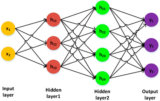
FIGURE 1. The calculation process of MLP.

We generally use the FC structure to conduct forward conduction in the calculation process. The specific calculation in “Hidden layer1” is expressed as follows:

${\mathit{h}}_{\mathbf{11}}=\mathit{\sigma }\left(\sum _{\mathit{i}=\mathbf{1}}^{\mathit{n}}{\mathit{w}}_{\mathbf{1}\mathit{i}}^{\mathbf{1}}{x}_{\mathit{i}}+{\mathit{b}}_{\mathbf{1}}\right)=\mathit{\sigma }\left({\mathit{w}}_{\mathbf{11}}^{\mathbf{1}}{x}_{\mathbf{1}}+{\mathit{w}}_{\mathbf{12}}^{\mathbf{2}}{x}_{\mathbf{2}}+{\mathit{b}}_{\mathbf{11}}^{\mathbf{1}}\right)(1)$

${\mathit{h}}_{\mathbf{12}}=\mathit{\sigma }\left(\sum _{\mathit{i}=\mathbf{1}}^{\mathit{n}}{\mathit{w}}_{\mathbf{2}\mathit{i}}^{\mathbf{1}}{x}_{\mathit{i}}+{\mathit{b}}_{\mathbf{1}}\right)=\mathit{\sigma }\left({\mathit{w}}_{\mathbf{21}}^{\mathbf{1}}{x}_{\mathbf{1}}+{\mathit{w}}_{\mathbf{22}}^{\mathbf{1}}{x}_{\mathbf{2}}+{\mathit{b}}_{\mathbf{21}}^{\mathbf{1}}\right)(2)$

${\mathit{h}}_{\mathbf{13}}=\mathit{\sigma }\left(\sum _{\mathit{i}=\mathbf{1}}^{\mathit{n}}{\mathit{w}}_{\mathbf{3}\mathit{i}}^{\mathbf{1}}{x}_{\mathit{i}}+{\mathit{b}}_{\mathbf{1}}\right)=\mathit{\sigma }\left({\mathit{w}}_{\mathbf{31}}^{\mathbf{1}}{x}_{\mathbf{1}}+{\mathit{w}}_{\mathbf{32}}^{\mathbf{1}}{x}_{\mathbf{2}}+{\mathit{b}}_{\mathbf{31}}^{\mathbf{1}}\right)(3)$

According to Eqs 1–3, when we need to synthesize the features extracted from the previous layer, each node of the FC layer is connected with all nodes of the upper layer. So, the FC networks make the best use of information from the previous layer but have the most parameters. It is suitable for small input and output. In order to simplify the expression of calculation. We use a matrix to express the process as follows:

${\mathit{H}}_{\mathbf{1}}=\left[\begin{array}{c}{\mathit{h}}_{\mathbf{11}}\\ {\mathit{h}}_{\mathbf{12}}\\ {\mathit{h}}_{\mathbf{13}}\end{array}\right]=\mathit{\sigma }\left(\left[\begin{array}{cc}{\mathit{w}}_{\mathbf{11}}^{\mathbf{1}}& {\mathit{w}}_{\mathbf{12}}^{\mathbf{1}}\\ {\mathit{w}}_{\mathbf{21}}^{\mathbf{1}}& {\mathit{w}}_{\mathbf{22}}^{\mathbf{1}}\\ {\mathit{w}}_{\mathbf{31}}^{\mathbf{1}}& {\mathit{w}}_{\mathbf{32}}^{\mathbf{1}}\end{array}\right]\left[\begin{array}{c}{\mathit{x}}_{\mathbf{1}}\\ {\mathit{x}}_{\mathbf{2}}\end{array}\right]+\left[\begin{array}{c}{\mathit{b}}_{\mathbf{11}}^{\mathbf{1}}\\ {\mathit{b}}_{\mathbf{21}}^{\mathbf{1}}\\ {\mathit{b}}_{\mathbf{31}}^{\mathbf{1}}\end{array}\right]\right)=\mathit{\sigma }\left({\mathit{W}}_{\mathbf{1}}\mathit{X}+{\mathit{b}}_{\mathbf{1}}\right)(4)$

Where the variable H₁ is the hidden layer output, and X is the input data. The variables W₁ and b₁ are the trainable weights decided in the training process. The function $\sigma$ is an activation operation that gives the model some nonlinear expression ability. Similar to Eq. 4, we define the output of “Hidden layer two” as H₂, the final output is Y, and the value can be calculated by:

${\mathit{H}}_{\mathbf{2}}=\mathit{\sigma }\left({\mathit{W}}_{\mathbf{2}}{\mathit{H}}_{\mathbf{1}}+{\mathit{b}}_{\mathbf{2}}\right),(5)$

$\mathit{Y}=\mathit{\sigma }\left({\mathit{W}}_{\mathbf{3}}{\mathit{H}}_{\mathbf{2}}+{\mathit{b}}_{\mathbf{2}}\right),(6)$

Similar to Eq. 4. The variables W₂, W₃, b₂, and b₃ are the trainable weights decided in the training process. According to Eqs 4–6, we can see that the output data of previous layers is the input data of this layer in networks. In this way, we can constantly extract new features by increasing the number of layers in the network.

In Eqs 4–6. We all need an activation function ($\sigma$). Activation functions are essential for artificial neural network models to learn and understand complex and nonlinear functions. Suppose we do not use the activation functions. In that case, each layer is the linear relationship between the input and output, and no matter how many layers there are in the neural network, the output always is a linear combination of the input. Using linear relations to estimate the change between input and output is unreasonable. So, we introduce a nonlinear factor to the neuron. It makes neural networks approach any nonlinear function arbitrarily so that neural networks can be applied to many nonlinear models. In our model, we use Parametric Rectified Linear Unit (PReLU), a member of the corrected Linear function (Leaky ReLU). The definition of PReLU is as follows:

$\mathit{P}\mathit{R}\mathit{e}\mathit{L}\mathit{U}\left(\mathit{x}\right)=\{\begin{array}{cc}\mathit{x},& \mathit{i}\mathit{f}\mathit{x}\ge \mathbf{0}\\ \mathit{a}\mathit{x},& \mathit{o}\mathit{t}\mathit{h}\mathit{e}\mathit{r}\mathit{w}\mathit{i}\mathit{s}\mathit{e}\end{array}(7)$

According to Eq. 7, when the input variable $\mathit{x}\ge \mathbf{0}$, the gradient of PReLU is a. It can avoid the phenomenon that the gradient is 0 on negative numbers and solve the gradient not updating problem. At the same time, slope a can also be learned in model training to reduce the trouble caused by artificial settings.

In order to better build the model and increase the convergence rate, the batch normalization (BN) method is also used after FC layers. The primary purpose of BN is to normalize the learned features into the specified distribution. It can be used to increase the convergence speed of learning and reduce the occurrence of the over-fitting phenomenon. The calculation process is as follows:

${\mathit{\mu }}_{\mathit{b}}=\frac{\mathbf{1}}{\mathit{m}}\sum _{\mathit{i}=\mathbf{1}}^{\mathit{m}}{\mathit{x}}_{\mathit{i}},(8)$

${\mathit{\sigma }}_{\mathit{b}}^{\mathbf{2}}=\frac{\mathbf{1}}{\mathit{m}}\sum _{\mathit{i}=\mathbf{1}}^{\mathit{m}}{\left({\mathit{x}}_{\mathit{i}}-{\mathit{\mu }}_{\mathit{b}}\right)}^{\mathbf{2}},(9)$

${\stackrel{\sim }{\mathit{x}}}_{\mathit{i}}=\frac{{\mathit{x}}_{\mathit{i}}-{\mathit{\mu }}_{\mathit{b}}}{\sqrt{{\mathit{\sigma }}_{\mathit{b}+\mathit{ϵ}}^{\mathbf{2}}}},(10)$

${\mathit{y}}_{\mathit{i}}=\mathit{\gamma }{\stackrel{\sim }{x}}_{\mathit{i}}+\mathit{\beta }=\mathit{B}{\mathit{N}}_{\mathit{\gamma },\mathit{\beta }}\left({\mathit{x}}_{\mathit{i}}\right),(11)$

Where the variable m represents the size of the batch, the variables $\gamma$ and $\beta$ are the weights decided in the training process.

Based on the introduction above, we use the structure of “FC + BN + PReLU” to construct the minimum cell of feature extraction. The network structure of our surrogate model is shown in Figure 2. The whole model is composed of five large layers. The first four layers (L1, L2, L3, and L4) are constructed by “FC + BN + PReLU”; their dimensions are L1 = 32, L2 = 64, L3 = 512, and L4 = 256, respectively. The last layer is only an FC layer with the dimension of L5 = N*M. It is used to map high-dimensional features to the dimensions of the output. In the last layer, N represents the number of nodes in the pipeline that need to be output, and M represents the properties (gas flow, oil flow, water flow, temperature, and pressure) that need to be simulated for each node. This structure can effectively simulate the pipeline change based on the surrogate model.

FIGURE 2

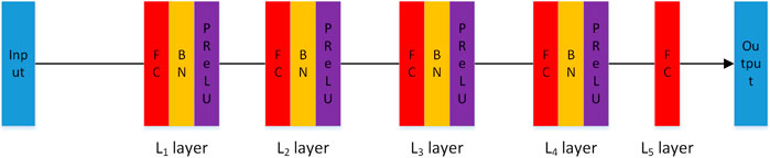
FIGURE 2. The detailed structure of the surrogate model.

2.2 Loss function and data preprocessing

In deep learning, we often use reverse conduction to optimize model parameters, so we set a standard to measure the quality of the training process, which refers to the loss function. The training objective is to minimize the metric between full-physics model production and prediction production during the offline stage. In this case, the simulation results are gas flow, oil flow, water flow, temperature, and pressure. So, in order to quantify the model’s overall performance in predicting the output state variables, we divide the total loss function into five parts: gas flow loss (Lg), oil flow loss (Lo), water flow loss (Lw), temperature loss (L_T) and pressure loss (Lp). Those specific definitions are as follows:

${\mathit{L}}_{\mathit{g}}=\frac{1}{\mathit{N}}\sum _{\mathit{i}=\mathbf{1}}^{\mathit{N}}{\left\{\sum _{\mathit{k}=\mathbf{1}}^{{\mathit{n}}_{\mathit{w}}}{\mathit{\mu }}_{\mathit{\kappa }}^{\mathit{g}}\Vert {\mathit{g}}_{\mathit{k}}-{\widehat{\mathit{g}}}_{\mathit{k}}\Vert \right\}}_{\mathit{i}},(12)$

${\mathit{L}}_{\mathit{o}}=\frac{1}{\mathit{N}}\sum _{\mathit{i}=\mathbf{1}}^{\mathit{N}}{\left\{\sum _{\mathit{k}=\mathbf{1}}^{{\mathit{n}}_{\mathit{w}}}{\mathit{\mu }}_{\mathit{\kappa }}^{\mathit{g}\mathit{o}}\Vert {\mathit{o}}_{\mathit{k}}-{\widehat{\mathit{o}}}_{\mathit{k}}\Vert \right\}}_{\mathit{i}},(13)$

${\mathit{L}}_{\mathit{w}}=\frac{1}{\mathit{N}}\sum _{\mathit{i}=\mathbf{1}}^{\mathit{N}}{\left\{\sum _{\mathit{k}=\mathbf{1}}^{{\mathit{n}}_{\mathit{w}}}{\mathit{\mu }}_{\mathit{\kappa }}^{\mathit{g}\mathit{w}}\Vert {\mathit{w}}_{\mathit{k}}-{\widehat{\mathit{w}}}_{\mathit{k}}\Vert \right\}}_{\mathit{i}},(14)$

${\mathit{L}}_{\mathit{T}}=\frac{1}{\mathit{N}}\sum _{\mathit{i}=\mathbf{1}}^{\mathit{N}}{\left\{\sum _{\mathit{k}=\mathbf{1}}^{{\mathit{n}}_{\mathit{w}}}{\mathit{\mu }}_{\mathit{\kappa }}^{\mathit{T}}\Vert {\mathit{T}}_{\mathit{k}}-{\widehat{\mathit{T}}}_{\mathit{k}}\Vert \right\}}_{\mathit{i}},(15)$

${\mathit{L}}_{\mathit{p}}=\frac{1}{\mathit{N}}\sum _{\mathit{i}=\mathbf{1}}^{\mathit{N}}{\left\{\sum _{\mathit{k}=\mathbf{1}}^{{\mathit{n}}_{\mathit{w}}}{\mathit{\mu }}_{\mathit{\kappa }}^{\mathit{p}}\Vert {\mathit{p}}_{\mathit{k}}-{\widehat{\mathit{p}}}_{\mathit{k}}\Vert \right\}}_{\mathit{i}},(16)$

We use variables without ‘hats’ to denote the proper solution (e.g., $go,w,Tandp$) and the variables with ‘hats’ to designate solutions approximated by the surrogate model (e. g., $\widehat{g}\widehat{o},\widehat{w},\widehat{T}and\widehat{p}$). The variable N represents the total number of training data sets and n_w is all output pipeline nodes, g represents gas flow rate, o represents oil flow rate, w represents water flow rate, T represents temperature, and p represents pressure. The variable ${\mu }^w$ ($\omega =go,w,Tandp$) is a transformable weight, and the values are decided by the actual input data. In this paper, those are calculated by:

${\mu }^{\omega }\left(x\right)=\{\begin{array}{cc}1,& ifx\ge 1e-3\\ 1/x,& ifx<1e-3\end{array},(17)$

According to Eq. 17, we can dynamically modify each node’s weight and increase the smaller data’s contribution to the loss. In this way, we also can avoid errors caused by large values eating small values in total loss. According to Eqs 12–16, the final total loss function is as follows:

$L_{all}=\lambda L_g+\beta L_o+\alpha L_w+\delta L_T+\mu L_p(18)$

In the flow process, due to the small range of temperature and pressure, the regression difficulty is relatively small, so the weight setting of this part is relatively minor. At the same time, due to the broader range of gas flow change (10,000 m³/day-m³/day) and close attention, we set the weight of gas loss as the maximum. The weights are λ = 50, β = 1, α = 1, δ = 1, μ = 1.

Data preprocessing is essential for the practical training of deep neural networks. Constraining training data values to be near zero with proper data normalization can enhance deep neural network training in many cases. In this study, the input data of the surrogate model are the gas flow rate, oil flow rate, water flow rate, temperature, and the pressure of the terminal (pipe network endpoint). At the same, the output is the change of gas flow rate, oil flow rate, water flow rate, temperature, and pressure at each point along the line. Due to differences in data units and actual production, the range of variation between different data is enormous. In order to improve the learning process and output quality, we need to normalize the input data. The normalization method is as follows:

${\alpha }^0=\frac{\alpha -0.001{\alpha }_{\mathit{min}}}{100\ast {\alpha }_{\mathit{max}}-0.001\ast {\alpha }_{\mathit{min}}},(19)$

The variable $\alpha$ represents the value of each variable in the pipeline, the variable ${\alpha }^0$ is the value after normalization, the variable ${\alpha }_{\mathit{min}}$ is the lower boundary of that variable, and ${\alpha }_{\mathit{max}}$ is the maximum observable value of that variable. In this paper, to ensure the range of data is [0,1] in the generalization, we use 100 and 0.001 to expand the limitation of max and min data.

3 Network simulation

3.1 The introduction of example

The gas field group in the eastern part of the South China Sea comprises one gas field and two pipelines (Figure 3). Gas file A is the deep-water gas field developed by underwater wellhead + marine pipe connection. In this gas file, we have two wells, A1 and A2, and the gas produced by those wells is transported downstream for further processing by pipeline (Gas file A to Platform1, Platform1 to Platform2, and Platform2 to terminal). In this gas field group, the driving types of gas reservoirs are diverse, the size of pipes are wildly different, and the coordination degree is low. At the same time, the flow simulation in pipelines is challenging due to the influence of downstream gas fluctuation. Therefore, under such a complex background, it is significant to simulate the flow of pipe networks quickly and accurately. Based on the actual pipe network flow of the gas field group, this paper simulated the internal flow condition for three pipelines in Figure 3. In order to introduce the result of our surrogate model in pipeline simulation, we use Gas file A to Platform1 as an example for a detailed description.

FIGURE 3

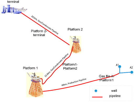
FIGURE 3. Production device layout of gas field group.

The total length of the sea pipe of gas file A to platform 1 is about 24 km, and an output point is taken every 2km, so there are 13 output nodes (including the beginning and end). In the data preparation stage, we first used LedaFlow to simulate the pipeline (see Figure 4 for the model). We then built multi-case numerical models based on the actual production data of the pipeline in 2015, 2019, and 2020. The range of input data of multiple calculation examples is shown in Table 1.

FIGURE 4

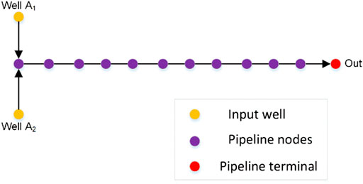
FIGURE 4. LeadFlow model of gas field pipeline.

TABLE 1

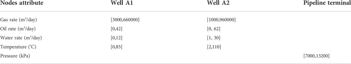
TABLE 1. The input data range of pipeline simulation for multi-example.

According to table 1, we can see that the input data is constructed by the gas rate, the water rate, the oil rate, the temperature, and the pressure of the endpoint of the pipeline. So, the input data is a 1D vector with nine elements. In data preprocessing, we first produced 215690 calculation examples with the random number within the specified range. Then, we first use the commercial software LeadFlow to get the result of every node in the pipeline and use Eq. 19 to deal with the data set. Finally, we use 80% of the data (172552) as the training set and 20% of the data (43,138) as the test set to train and test the model.

The training of the surrogate model can be accomplished efficiently, though the specific training time depends on many factors. These include the training data, training set size, batch size, optimizer setup, learning rate, and the graphics processing unit (GPU) performance. Through the numerical experiments, the weights of those losses are λ = 50, β = 1, α = 1, δ = 1, μ = 1. The most effective optimizer is Adam; the initial learning rate is 0.00001. Regarding time, our training process converges in 240 min on an RTX2060 GPU using Tensorflow. The convergence process of the total loss on both training and testing data sets is presented in Figure 5. It shows that the losses converge quickly after 40 epochs of training, and the trend and value are both similar for training and testing data sets, indicating that the optimal hyper parameters are credible with no problem of overfitting.

FIGURE 5

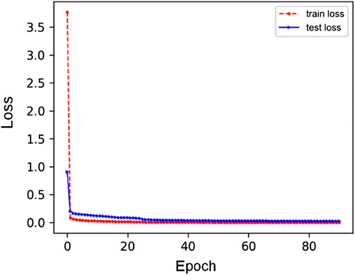
FIGURE 5. The convergence trend of total loss in train and test (red line is train process, the blue line is test process).

4 Result of test case

In this part, we mainly analyze the simulation results. Without losing any generality, we pick the outputs from one test case for a detailed description, and the test results are shown in Figures 6–10. In the figures, the green dotted line represents LeadFlow results; the red line represents our surrogate model results. We can see that our model results and the commercial software LeadFlow have the exact change trend. In numerical, our model results closely match the results from LeadFlow simulations in temperature and some more enormous differences in pressure, gas rate, oil rate, and water for all nodes.

FIGURE 6

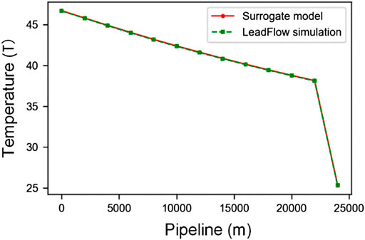
FIGURE 6. The change of temperature along the pipeline between surrogate mode and LeadFlow simulation.

FIGURE 7

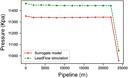
FIGURE 7. The change of pressure along the pipeline between surrogate mode and LeadFlow simulation.

FIGURE 8

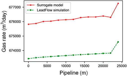
FIGURE 8. The change of gas rate along the pipeline between surrogate mode and LeadFlow simulation.

FIGURE 9

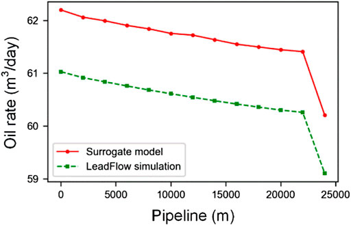
FIGURE 9. The change of oil rate along the pipeline between surrogate mode and LeadFlow simulation.

FIGURE 10

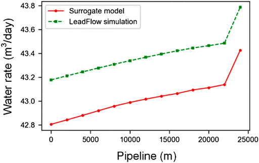
FIGURE 10. The water rate change along the pipeline between surrogate mode and LeadFlow simulation.

In order to metric the degree of difference in numerical, we calculate the relative error through Eqs 20–22.

${\mathit{E}}_{\mathit{j}}^{\mathit{k}}=\frac{1}{\mathit{N}}\sum _{\mathit{i}=\mathbf{1}}^{\mathit{N}}\Vert {\mathit{y}}_{\mathit{j}}^{\mathit{i}\mathit{k}}-{\widehat{\mathit{y}}}_{\mathit{j}}^{\mathit{i}\mathit{k}}\Vert ,(20)$

${\mathit{P}}_{\mathit{j}}^{\mathit{k}}=\frac{1}{\mathit{N}}\sum _{\mathit{i}=\mathbf{1}}^{\mathit{N}}\Vert {\mathit{y}}_{\mathit{j}}^{\mathit{i}\mathit{k}}\Vert ,(21)$

${\mathit{R}\mathit{E}}_{\mathit{j}}^{\mathit{k}}=\frac{{\mathit{E}}_{\mathit{j}}^{\mathit{k}}}{{\mathit{P}}_{\mathit{j}}^{\mathit{k}}},(22)$

Where k represents nodes, J represents attributes (gas, oil, water, temperature, and pressure), and N represents the number of all test sets. The variable y indicates the solution of the LeadFlow simulation, $\widehat{y}$ is the result of the surrogate model. The variable $E_j^k$ indicates the average absolute error of the attribute j at the node k for all test sets, and $P_j^k$ indicates the average value of attribute j at the node k for all test sets. $R{E}_j^k$ represents the average relative error of the attribute j at the node k for all test sets.

In order to illustrate that the results of our surrogate model and full-physics model are close, we calculate the relative errors for pressure, gas rate, oil rate, and water for all nodes using Eqs 20–22 in the above test case. In this way, we get the max relative error in pressure is 0.42%, the gas rate is 0.44%, the oil rate is 1.63%, and the water rate is 1.36%. So, it proves that our model has good accuracy.

In order to avoid sampling differences, we will analyze the general performance for all test cases. We calculate the relative error for every case using Eqs 20–22 with N = 1. The result is shown in Figure 11. The orange line in the center of each box represents the median error; the bottom and top edges of the box represent the 25th and 75th percentile errors; the “whiskers” protruding from the box represents the minimum and maximum errors. Though the oil rate’s relative error is higher than others, the overall errors are both low, and the max value is about 6.01%. In terms of numerical results, the medial relative error for temperature is 0.56%, pressure is 0.79%, gas rate is 1.02%, oil rate is 1.85%, and water rate is 0.80%.

FIGURE 11

FIGURE 11. The distribution of relative error for all test cases and nodes.

In Figure 11, the green circle is the average error for all cases and nodes. In order to metric average relative errors for all cases, we use N = 43,138 in Eqs 20–22. The result is shown in Figure 12. It can be seen from the figure that the relative errors of the results obtained by our surrogate model are all low, and the max value is about 2%. Therefore, our model has a specific guiding value in actual production.

FIGURE 12

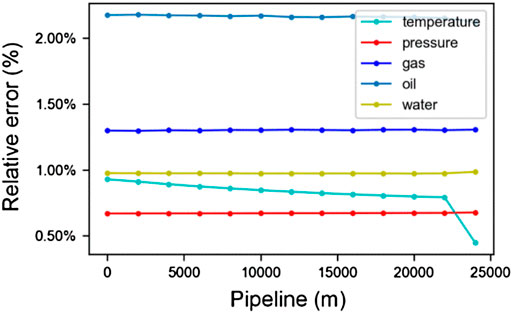
FIGURE 12. The average relative error for all test cases at different nodes.

4.1 Computing speed

In this part, we mainly discuss the time costs of LeadFlow simulation and our surrogate model. LedaFlow usually simulates a case with 10 s on Intel Xeon (R) W-3275m dual CPU with 28 cores machine. However, it has complex concurrency, and the run time is unstable. The convergence of the entire simulation may take about 22 s when we use some special parameter settings. On an RTX2060 GPU node with 6 GB video memory, our surrogate model can run 16 examples in 0.15 s, and the average time of each example is 0.008 s (8 ms), and the speed is nearly 1,250 times higher.

5 Conclusion

In this work, we propose a surrogate model with MLP to solve the problem of pipeline simulation on gas transport. We use “FC + BN + PReLU” to construct the surrogate model. In the training process, the weights of the loss function are dynamically decided by the input data value. We use our model in an existing pipe network. Compared with traditional LedaFlow, the max relative error is about 6%, and our model’s average relative errors are below 2%. In addition, the trend of our simulation results is highly consistent with LedaFlow simulation results, and our model can provide about 1,250 times acceleration. In summary, our surrogate model could provide a highly accurate and super-fast surrogate for a realistic pipeline system. The model could be beneficial when a large amount of simulation runs is required for allocation of optimization.

Future research is to be carried out from two aspects. First, we would expand this model to deal multi pipelines with one model because there are many pipelines in realistic gas transport. If we construct a model for every pipeline, we need many models, which are expensive for the hardware. Second, we are interested in building an integrated model for the gas reservoir and pipeline network, which can automatically simulate the pipeline flow changes caused by any gas reservoir changes.

Data availability statement

The raw data supporting the conclusion of this article will be made available by the authors, without undue reservation.

Author contributions

All authors contributed to the article and approved the submitted version.

Conflict of interest

Authors FQ, ZY, PY, ST and HH were employed by the company CNOOC Ltd. -SHENZHEN.

Publisher’s note

All claims expressed in this article are solely those of the authors and do not necessarily represent those of their affiliated organizations, or those of the publisher, the editors and the reviewers. Any product that may be evaluated in this article, or claim that may be made by its manufacturer, is not guaranteed or endorsed by the publisher.

References

Al-Sarkhi, A., and Hanratty, T. J. (2002). Effect of pipe diameter on the drop size in a horizontal annular gas–liquid flow. Int. J. Multiph. flow 28 (10), 1617–1629. doi:10.1016/S0301-9322(02)00048-4

CrossRef Full Text | Google Scholar

Aman, Z. M., Di Lorenzo, M., Kozielski, K., Koh, C. A., Warrier, P., Johns, M. L., et al. (2016). Hydrate formation and deposition in a gas-dominant flowloop: Initial studies of the effect of velocity and subcooling. J. Nat. Gas Sci. Eng. 35, 1490–1498. doi:10.1016/j.jngse.2016.05.015

CrossRef Full Text | Google Scholar

AUNICKY, Z. (1970). The longitudinal mixing of liquids flowing successively in pipelines. Can. J. Chem. Eng. 48 (1), 12–16. doi:10.1002/cjce.5450480103

CrossRef Full Text | Google Scholar

Bruyelle, J., and Guérillot, D. (2019). “Proxy model based on artificial intelligence technique for history matching-application to brugge field,” in SPE Gas & Oil Technology Showcase and Conference. OnePetro. doi:10.2118/198635-MS

CrossRef Full Text | Google Scholar

de Freitas Rachid, F. B., Carneiro de Araujo, J. H., and Baptista, R. M. (2002). The influence of pipeline diameter variation on the mixing volume in batch transfers. Int. Pipeline Conf. 36207, 997–1004. doi:10.1115/IPC2002-27168

CrossRef Full Text | Google Scholar

Gers, F. A., Schmidhuber, J., and Cummins, F. (2000). Learning to forget: Continual prediction with LSTM. Neural Comput. 12 (10), 2451–2471. doi:10.1162/089976600300015015

PubMed Abstract | CrossRef Full Text | Google Scholar

Kang, P. S., Lee, D. G., and Lim, J. S. (2014). “Status of wax mitigation technologies in offshore oil production,” in The Twenty-fourth International Ocean and Polar Engineering Conference, Busan, Korea, June 15–20, 2014. OnePetro.

Google Scholar

Laín, S., and Sommerfeld, M. (2012). Numerical calculation of pneumatic conveying in horizontal channels and pipes: Detailed analysis of conveying behaviour. Int. J. Multiph. Flow 39, 105–120. doi:10.1016/j.ijmultiphaseflow.2011.09.006

CrossRef Full Text | Google Scholar

Marfatia, Z., and Li, X. (2022). On steady state modelling for optimization of natural gas pipeline networks. Chem. Eng. Sci. 255, 117636. doi:10.1016/j.ces.2022.117636

CrossRef Full Text | Google Scholar

Rachid, F. F., de Araujo, J. C., and Baptista, R. M. (2002). Predicting mixing volumes in serial transport in pipelines. J. Fluids Eng. 124 (2), 528–534. doi:10.1115/1.1459078

CrossRef Full Text | Google Scholar

Spandonidis, C., Theodoropoulos, P., Giannopoulos, F., Galiatsatos, N., and Petsa, A. (2022). Evaluation of deep learning approaches for oil & gas pipeline leak detection using wireless sensor networks. Eng. Appl. Artif. Intell. 113, 104890. doi:10.1016/j.engappai.2022.104890

CrossRef Full Text | Google Scholar

Tang, M., Liu, Y., and Durlofsky, L. J. (2020). A deep-learning-based surrogate model for data assimilation in dynamic subsurface flow problems. J. Comput. Phys. 413, 109456. doi:10.1016/j.jcp.2020.109456

CrossRef Full Text | Google Scholar

Wang, Z., Xiao, D., Fang, F., Govindan, R., Pain, C. C., and Guo, Y. (2018). Model identification of reduced order fluid dynamics systems using deep learning. Int. J. Numer. Methods Fluids 86 (4), 255–268. doi:10.1002/fld.4416

CrossRef Full Text | Google Scholar

Xie, Y., Meng, J., and Chen, D. (2022). Wax deposition law and OLGA-Based prediction method for multiphase flow in submarine pipelines. Petroleum 8 (1), 110–117. doi:10.1016/j.petlm.2021.03.004

CrossRef Full Text | Google Scholar

Xiong, J., Liang, W., Liang, X., and Yao, J. (2022). Intelligent quantification of natural gas pipeline defects using improved sparrow search algorithm and deep extreme learning machine. Chem. Eng. Res. Des. 183, 567–579. doi:10.1016/J.CHERD.2022.06.001

CrossRef Full Text | Google Scholar

Zhou, D., Jia, X., Ma, S., Shao, T., Huang, D., Hao, J., et al. (2022). Dynamic simulation of natural gas pipeline network based on interpretable machine learning model. Energy 253, 124068. doi:10.1016/j.energy.2022.124068

CrossRef Full Text | Google Scholar