Optimization of temperature distribution in the novel power-to-heat matrix-in-batch OnePot© reactor

In this work, we assess the optimal temperature distribution inside a new automated, stand-alone, matrix-in-batch patented reactor, named OnePot^©. This novel reactor is equipped with seven rotating hot rotating cylinders—here referred to as spots—which make it possible a precise tuning of fluid temperature. To conduct this investigation, we consider two radial layout of spots, here indicated as uniform configuration and alternate one, respectively. The former characterised by a single uniform equilateral triangular pitch, whereas the latter by two different equilateral triangular pitches alternated to form a double-triangle star. We consider two different fluids, water and argon, as representative of the behaviour of liquids and gases, respectively. Furthermore, the effect of viscosity is also taken into account by forcefully increasing that of water by 100 and 1,000 times. The optimization of the temperature distribution is performed obtaining velocity and temperature fields using a computational fluid dynamic (CFD) approach. As a sort of objective function to maximise, we defined a thermal mixing efficiency to provide a quantitative measure of the temperature distribution uniformity. As a remarkable result, we find an optimal value of pitch approximately equal to 36% of the vessel diameter for both liquid water and argon gas. As for the alternate configuration, we found that it provides a better temperature distribution than the uniform one, especially at high viscosity values. This is because the inner spots are able to prevent the formation of large colder “islands” around the centre. Furthermore, we estimate the overall heat transfer coefficient between thermal spots and fluid bulk, whose values are perfectly in line with the literature ones. The modularity of our novel fully-electric reactor allows for applications in a number of industrial contexts, especially pharmaceutical ones.

1 Introduction

The efficiency of transport phenomena related to heat and mass transfer between chemicals are crucial for a successful design of a chemical process, both at laboratory and industrial scale. Batch reactors are the most used reactor type for industrial production of chemical commodities, fine chemicals and pharmaceuticals, whose sectors are essentially differentiated by their production volumes.

Batch reactors consist in closed vessels, often pressurized, equipped with integrated heating/cooling systems and agitators. Heat transfer efficiency, safety and homogeneity inside huge volumes of chemicals, mixed in a batch reactor, is a challenge for the modern chemical industry, especially from the sustainability point of view.

Traditionally, heat transfer in chemical reactors is usually achieved by heat exchange with a medium (i.e., a vapour steam) heated by burning fossil fuels. The heat transfer could be practically realized by either jacket vessels or external heater exchangers.

Alternatively, resistive coils could be used to heat the vessel from inside (Silla, 2003). All these approaches suffer from both fundamental and ecological issues: firstly, heating a huge volume by a superficial approach involves convective heating mechanisms to reach the homogeneity, with low energy efficiency, long reaction time and low quality of the final products.

Besides, the use of fossil fuels as energy sources is no longer acceptable for production industries because of the urgent need of mitigating CO₂ emissions. The progressive electrification of productive sectors, in terms of both generating electricity from renewable sources and use only electricity as source of process heating, is proposed as the most reliable alternative to reach the sustainability goal (Bran et al., 2010).

Nowadays, several different power-to-heat technologies, where heating is essentially due to a Joule effect by the object where the electricity pass through, are available, at least on laboratory scale, with some of them being scaled-up to industrial level. Such technologies can be differentiated in direct or indirect, depending on if the heat is generated directly in the reaction bulk, or indirectly on a conductive object in contact with the reaction vessel.

While indirect heating still not solve the problem of convective inefficiency, direct technologies could provide interesting solutions for effective heating transfer and homogeneity (Kim et al., 2022; Son et al., 2022). Figure 1 offers a representation of direct power-to-heat technologies, which were verified at least at laboratory scale. Inductive, Ohmic and Microwaves heating are schematically presented by pointing out the unicity points of each technology compared to conventional heating (Figure 1A).

FIGURE 1

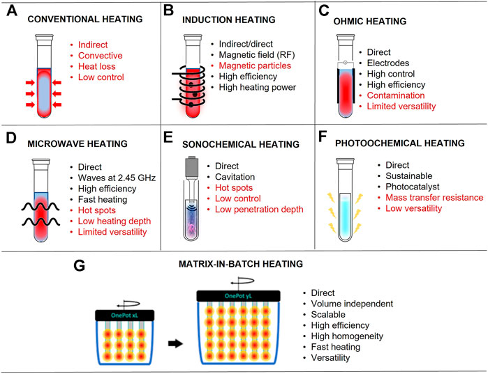
FIGURE 1. Schematic representation of Matrix-in-Batch heatingtechnology compared to other direct-heating methods.

Besides them, two other alternative heating sources to realize direct heating for chemical transformation are reported, namely sonochemical and photochemical heating systems. Each of them successfully approached the challenge of sustainability energy production and transferring.

Nevertheless, they all have fundamental and/or technical limitations in terms of either scalability or versatility. The Inductive Heating (Figure 1B) exploits magnetic fields generated in the range of radiofrequency to heat magnetic particles inside the vessels: the particles act as heat-transfer, practically not eliminating the heat transfer problems to the surroundings (Houlding and Rebrov, 2012).

The Ohmic Heating (Figure 1C) consists in the application of a voltage to electrodes directly immersed into the reaction bulk; the heating is due to the friction generated by ion movement: in this case good homogeneity and penetration are reached but the nature of electrodes must be carefully customized depending on the applications (Silva et al., 2017; Turgut et al., 2022).

The Microwave Heating (Figure 1D) is based on the exposure of the reaction bulk to microwaves, thus generating heat by both dipolar polarization mechanism and ionic ionization mechanism; the speed of heating is the principal advantage of the technology, limited by the low penetration depth in huge volumes (Siddique et al., 2022). Moreover, both Ohmic and Microwaves Heating are limited by the dielectric nature of the medium.

The Sonochemical Heating (Figure 1E) is based on the generation of an acoustic wave inside the bulk, going up to dilatation and rarefaction cycles, originating collapsing bubbles acting as hot spots inside the medium. Such a technology, as well as the Microwaves Heating, has the problem of heating inhomogeneity.

Finally, Photochemical Heating (Figure 1F) exploits the most sustainable source of energy, solar energy, to heat photochemical absorbers, often acting as reaction catalysts, to activate the process. The main limit of this technology is that essentially only redox reactions can be photochemically activated, with an evident limit of versatility (Mandal, 2019; Belwal et al., 2020).

Starting from this evidence and looking for a direct heating technology able to solve at the time the need of efficiency, versatility, and scalability, we patented a new technology, named Matrix-in-Batch technology, schematically represented in Figure 1G. The heating source of this technology is the oldest direct power-to-heat technology, i.e. the resistance heating (Balakotaiah and Ratnakar, 2022), but we proposed a disruptive way to make the heating independent by the reaction volume.

The concept is to discretize the reaction volume into smaller, continuous volume cells, each of one being delimited by a matrix of points. Each matrix point is heated separately by a heating actuator and controlled by a retrofitting temperature sensor. Such set of active and passive elements were organized in cylinders named “spots”. The spots were anchored to the reactor vessel cup, named “reaction head” and immersed into the reaction bulk. The spots number can be tailored in function of the specific reaction volume, thus assuring rapid scalability. Moreover, the reactor head is able to rotate, thus generating reaction mixing and, consequently, heating homogeneity. The new batch reactor, integrating the matrix-in-batch technology, is patented with the name of OnePot^© (Francardi and Oliverio, 2021).

With the aim at studying the thermal performance of this novel reactor, in this paper, we present an assessment of optimal temperature distribution inside the reactor vessel by a 2-D computational fluid dynamic (CFD) simulations, which is performed to study the influence of the pitch on such a matrix-heating system. The details of the methodology followed in the present study are reported and described in the following sections.

2 Description of the system

Figure 2 shows a 3D scheme of the system considered in the present work, which is composed of seven vertical spots physically connected to a rotating disk. The transversal (radial) distribution of the spots is also a subject of investigation of the present work and, thus, we have analysed different configurations (see Section 4.1 for details). All the spots rotate with an angular velocity of 250 rpm inside a fixed vessel, which allows the fluid inside reactor to heat up/cool down progressively with the possibility of a precise temperature control. Moreover, such an angular velocity ensures that the reactor work in laminar conditions—maximum Reynolds number for water of 560 and for argon of 40 in all the conditions considered –, which allows us to control better the fluid dynamics of the system. We expect that the situation be more complex when working in turbulent regime (see, for example, Ma et al., 2015; Evrim et al., 2021; Zhao et al., 2022) and, thus, a dedicated analysis, which is out of the scope of the present study, is needed.

FIGURE 2

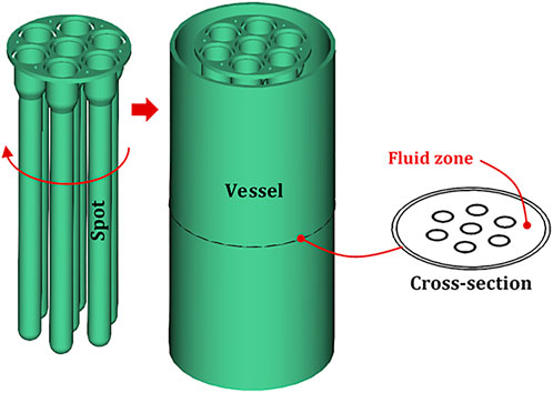
FIGURE 2. Sketch of the novel Matrix-in-Batch rotating reactor OnePot^© considered in the present work. The actual system subject of investigation is the fluid zone of the cross-section. The oriented red arrow near the spots indicates the sense of rotation.

As the length of the spots is much large than the distance between spots, for the purpose of this investigation, we analysed the thermo-fluid dynamics of the 2D cross-section, excluding in practice the boundary effects on the top and the bottom of the vessel, whose 3D domain is not a subject of this study.

3 Mathematical modelling

This section reports the details of the mathematical modelling related to momentum, heat and mass conservation as well as to the transport equations along with the required boundary conditions and computational settings.

3.1 Conservation and transport equations

The conservation equations for momentum are implemented through the Navier-Stokes equations along with the continuity equation (Eq. 1):

$\begin{array}{l}\rho \frac{\partial \underset{¯}{u}}{\partial t}+\rho \left(\underset{¯}{u}\cdot \nabla \right)\underset{¯}{u}=\nabla \cdot \left[-p\underset{¯}{\underset{¯}{I}}+\mu \left(\nabla \underset{¯}{u}+{\left(\nabla \underset{¯}{u}\right)}^T\right)-\frac{2}{3}\mu \left(\nabla \cdot \underset{¯}{u}\right)\underset{¯}{\underset{¯}{I}}\right]\\ \frac{\partial \rho }{\partial t}+\nabla \cdot \left(\rho \underset{¯}{u}\right)=0\end{array}(1)$

In addition, we pair the energy balance (Eq. 2):

$\rho C_p\frac{\partial T}{\partial t}+\rho C_p\left(\underset{¯}{u}\cdot \nabla T\right)=\nabla \cdot \left[-\underset{¯}{q}\right]+Q+W_p(2)$

We need to specify that, in the conditions considered in this investigation, the fluid dynamics is characterized by a laminar flow and, thus, no turbulence model is used.

As for transport models, the momentum and energy transfer for water and argon is described by Newton’s and Fourier’s law, respectively.

3.2 Initial and boundary conditions

The initial conditions in the whole domain for momentum consists in setting the velocity field to zero and pressure to the atmosphere (1 atm). As for the energy, we set the temperature at the surface of the spots $T_{spot}$ equal to 90°C and the temperature in the remaining domain to the external one T_ext = 25°C.

As for the boundary conditions for momentum, we set the no-slip condition both at the surface of the vessel and at the surface of the spots. However, the implementation of such a conditions at the surface of the spots is different from that at the vessel surface because the former rotate around the axis of the central spot, whereas the latter remains fixed. In particular, the following condition for the velocity field u is set at the walls of the rotating domain (Eqs 3, 4), which basically states the same velocity between fluid fillets adjacent to the rotating surface and the rotating surface itself:

$\underset{¯}{u}={\underset{¯}{u}}_{wall}={\left(\frac{\partial \underset{¯}{x}}{\partial t}\right)}_{\begin{array}{l}Rotating\\ walls\end{array}}(3)$

${\left(\frac{d\alpha }{dt}\right)}_{wall}={\omega }_{wall}=-2\pi f(4)$

The angular displacement represents an additional equation, corresponding to an additional dependent variable to solve for.

As for the boundary conditions for energy, the temperature at the surface of the spots $T_{spot}$ is fixed at the value of 90°C, whereas we set different heat flux values at the wall of the vessel depending on whether such a wall is considered adiabatic or not. In the former case, a null heat flux is set at the vessel wall (i.e., thermal insulation, Eq. (5)):

$-\underset{¯}{n}\cdot \left(-k\nabla T\right)=0(5)$

whereas, in the latter case (i.e., non-adiabatic conditions, Eq. 6), a non-null heat flux across the vessel wall is calculated through the product of an external free-convection heat transfer coefficient, estimated to be equal to 7 W s⁻¹ m⁻², and the difference between the external temperature $T_{ext}$ (constant) and the wall temperature $T_{wall}$ (changing with time), which is taken as the characteristic energy flux driving force:

$-\underset{¯}{n}\cdot \left(-k\nabla T\right)=h_{T,ext}\left[T_{ext}-T_{wall}\left(t\right)\right](6)$

3.3 Assessment of thermal efficiency

In the present work, the primary results are given in terms of 2-D temperature profiles in the fluid zone of the vessel. However, although very explicative on a visualization point of view, such profiles alone do not allow a quantitative analysis of the thermal distribution inside the system, which is the primary goal of the present investigation.

Therefore, we define the here-called thermal mixing efficiency η_T (Eq. 7), which is a parameter introduced here to measure quantitatively the uniformity of temperature distribution in the fluid.

${\eta }_T\equiv \frac{{\overline{T}}_{bulk}-T_{ext}}{T_{spot}-T_{ext}}(7)$

In particular, we define ${\eta }_T$ as the ratio of the difference between average bulk temperature ${\overline{T}}_{bulk}$ and external (nominal room) temperature $T_{ext}$ and the difference between spot temperature $T_{spot}$ and the external one. The genesis of such a definition is based on the following considerations.

If ${\overline{T}}_{bulk}$ tends to $T_{ext}$—which is the worst case with respect to the uniformity of temperature distribution—${\eta }_T$ tends to zero, this being the desired value actually corresponding to the worst distribution. If, on the other hand, ${\overline{T}}_{bulk}$ tends to $T_{spot}$—which is the best case with respect to the uniformity of temperature distribution—${\eta }_T$ tends to the unity, this being the desired value actually corresponding to the best distribution. These considerations are summarised mathematically in Eq. 8.

$\begin{array}{l}\{\begin{array}{l}{\eta }_T\left({\overline{T}}_{bulk}\to T_{ext}\right)\to 0\left(\mathrm{W}\mathrm{o}\mathrm{r}\mathrm{s}\mathrm{t}\mathrm{C}\mathrm{a}\mathrm{s}\mathrm{e}\right)\\ {\eta }_T\left({\overline{T}}_{bulk}=T_{spot}\right)=1\left(\mathrm{B}\mathrm{e}\mathrm{s}\mathrm{t}\mathrm{C}\mathrm{a}\mathrm{s}\mathrm{e}\right)\end{array}\\ \Downarrow \\ 0<{\eta }_T\le 1\end{array}(8)$

3.4 Assessment of heat transfer coefficient

Regarding the definition of an overall heat transfer coefficient $h_T$, we choose to assess it by considering the area of the spot surface $A_{spot}$ as the characteristic heat exchange area and, consequently, the total energy flux ${\dot{Q}}_{spot}$ (referred to both convective and conductive heat exchange modes) exchanged across the spot surface as the effective energy flux exchanged between spots and fluid.

As for the required characteristic temperature difference, we choose the difference between the spot temperature $T_{spot}$ and the bulk temperature averaged over the whole domain ${\overline{T}}_{bulk}$, which is chosen to be the nominal bulk temperature similarly to what done in previous works for different systems (Caravella et al., 2012; Caravella et al., 2016). The resulting definition of $h_T$ is eventually reported in Eq. 9.

$h_T\equiv \frac{{\stackrel{·}{Q}}_{spot}}{A_{spot}\left(T_{spot}-{\overline{T}}_{bulk}\right)}(9)$

4 Simulation settings

This section provides information on the computational settings required to carry out the simulation campaign in terms of construction of the computational mesh (Section 4.1) and solver settings (Section 4.2).

4.1 Computational mesh

As aforementioned, we have investigated different configurations relative to the radial distribution of pitch. In particular, we studied two configurations: 1) a first one, which has a uniform equilateral triangular pitch (Figure 3A)—here simply referred to as uniform configuration–and 2) the second one, characterised by three outer spots having a uniform equilateral triangular pitch with the central spot (namely pitch₁) alternated with other three inner spots having a uniform equilateral triangular pitch (namely pitch₂) with the central one (Figure 3B)—here simply referred to as alternate configuration.

FIGURE 3

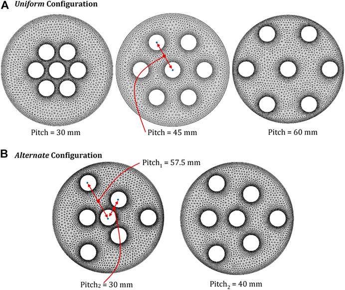
FIGURE 3. Example of computational mesh for (A) the uniform configurationand (B) the alternate configuration for different pitch values.

The study of the latter configuration has chronologically followed that of the former one, as the reason for its investigation has arisen from the analysis of some inefficiencies observed in the temperature distribution of the uniform configuration (see Section 5.2.1). In particular, we anticipate that, after finding the optimal pitch value for the uniform distribution (around 57.5 mm), in the alternate one we set the pitch₁ value equal to the optimal value, considering two values of pitch₂ (30 and 40 mm).

The construction of the computational mesh for the various geometry is made in the built-in tool available in COMSOL MULTIPHYSICS^®. The calibration of the elements size is tuned to balance the elements quality with the computational duty, which cannot be too high. The tuned meshing parameters are the following: 1) maximum element size, 2) minimum element size, 3) maximum element growth rate, 4) curvature factor and 5) resolution of narrow regions. In fact, it is suggestable to build a narrower mesh near the walls (highest gradients) and a coarser one in the fluid bulk to minimize the computational duty. Figure 3 shows examples of computational meshes built for three different pitch values. Table 1 reports the geometrical and physical parameters considered for the CFD simulation of the system along with the time range of investigation.

TABLE 1

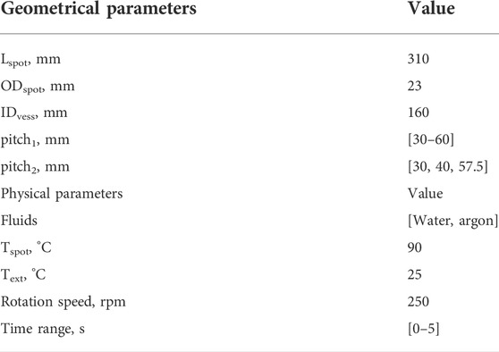
TABLE 1. Geometrical and physical parameters of the system.

4.2 Solver settings

As for the settings of the numerical solver, backward differentiation formulas (BDFs) with order of accuracy varying from one to five are used for simulation (but mainly the fully Euler backward scheme). To accelerate the convergence during the nonlinear iterations, the option “Anderson acceleration” is activated to control the number of iteration increments.

The solution process is split into sub-steps by using segregated solvers, whose strategy consists in solving iteratively each physics (angular displacement, momentum balance and energy balance, in this specific case) taking the profile of the physics not solved for from the previous iteration. The end-user can choose the order of the segregated solvers according to the complexity of the system. In this work, we choose the following order: 1) angular displacement, 2) momentum balance (i.e., velocity field and pressure) and 3) energy balance (i.e., temperature field).

End-users can also choose the linear solver required to solve the linear system associated to each segregated solver, which can be divided into two categories: direct solvers and iterative solvers. The former are faster but require a greater computational duty, whereas the latter are slower but need less amount of allocated memory.

In this specific case, we choose the direct solver PARDISO (PARallel sparse DIrect SOlver) to solve the angular displacement (segregated step 1) and temperature field (the segregated step 3), and the iterative solver GMRES (Generalized Minimum RESidual) for the velocity field (segregated step 2).

To further minimise the computational duty, a Geometric Multigrid Solver (GMS) is used, based on hierarchical multigrid levels, where each level corresponds to a mesh and to a particular choice of the shape functions. The number of degrees of freedom decreases at a coarser multigrid level.

The idea is to perform just a fraction of the computations on the fine mesh, performing computations on the coarser meshes when possible and leading in this way to a fewer number of operations.

5 Results and discussion

This section reports and discusses the results relative to the heating process conducted in the novel reactor for two fluids: water and argon, which are respectively taken as representatives of liquid and gas behaviour. In all simulations, the temperature of the spots and the initial temperature of the fluid are set to 90°C and 25°C, respectively, for both fluids. The former value is chosen to prevent water boiling, whereas the latter represents the typical value of room temperature. Simulations are all carried out in a time range of 0–5 s.

5.1 Validation of the spot surface temperature

Figure 4 shows the experimental monitoring of the time profile of the spot temperature $\left(T_{ext}\right)$ measured at two different positions–namely top and bottom–over the external surface. The trends after 20 s are steady and, thus, are not shown. Specifically, a temperature value of 70°C is set as input to the controller, adjusting the temperature at the inner centre of the spot $\left(T_{int}\right)$, which is higher than the surface temperature of 21–27°C due to the materials thermal resistance. A power of 7 W is supplied to both top and bottom power cells. The slight difference between the temperature values of top and bottom (around 3%) is due to a certain interference between inner heating cells of the matrix. As we can see from the plot, the surface temperature of the spot can be kept near the target value within the considered time range, this allowing us to consider a constant value at the spot surface for simulation.

FIGURE 4

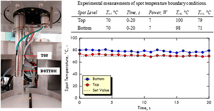
FIGURE 4. Experimental measurements of the time profile of the spot temperature.Temperature is measured at different positions over the spot surface, namely top and bottom.

5.2 Case study 1: Liquid water

This section reports the results relative to the water at different pitch configurations (uniform and alternate, respectively), pitch and viscosity values.

5.2.1 Uniform configuration

Figure 5 shows the temperature profiles for liquid water in uniform configuration at two different time values (1 and 5 s) and three different values of equilateral pitch (30, 45 and 60 mm) obtained in adiabatic conditions (more simulation videos are available in the Supplemental Material). Considering the time of 1 s, we can observe that, for the lowest pitch considered, the heating process is mainly concentrated in the centre of reactor, whereas, as expected, an increase of pitch moves progressively the heating zone towards the external wall. In particular, by looking at the 45 mm-pitch case, it is found that there are two cold zones: the first one between the spot in the centre and the surrounding ones, and the second one between the surrounding spots and the external wall.

FIGURE 5

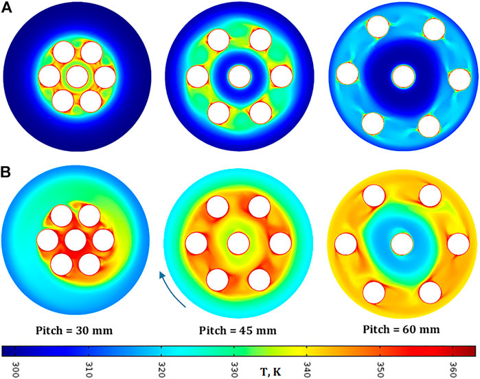
FIGURE 5. Temperature profiles at (A) 1s and (B) 5 s for different pitch values in adiabatic conditions in uniform configuration. Fluid: water, T_spot = 90°C, T_ext = 25°C.

For the other two cases, 30 mm and 60 mm, a single cold zone is found respectively towards the external wall and near the centre. This indicates that the heating process mainly occurs by convection along the trajectory of the spots and by conduction along the radial direction.

Furthermore, a higher pitch value seems to decrease the maximum temperature reached in the fluid but to increase the uniformity of temperature distribution along the spots trajectory. This is due to the higher distance between the spot surfaces, which makes the fluid heating less efficient.

Another interesting aspect to notice is the relatively symmetric characteristic of profiles at this time value, which does not seem much affected by the centrifugal force field induced by rotation. However, the situation is slightly different if looking at the profiles at 5 s, especially those for a pitch of 30 mm. In fact, it can be observed a clear sling effect of the centrifugal field in spreading the warm zone towards the external wall in form of spiral trail.

The same effect is also present in the temperature profiles related to the other two pitch values. However, for a pitch of 45 mm, it is mitigated by the proximity with the wall and with the central spot, whereas, for a pitch of 60 mm, the centrifugal force distorts the central cold zone breaking the profile symmetry.

In order to check the influence of the adiabatic condition, we also simulated the same systems depicted in Figure 5 in non-adiabatic conditions by using a typical value of the external heat transfer coefficient $h_{t,ext}$ for free convection (7 W m⁻² K⁻¹). The results of simulations show that the temperature profiles are approximately the same as those calculated in adiabatic conditions, this stating that this aspect does not influence the previous analysis.

As stated in the previous section, to assess the thermal efficiency in a quantitative way, we introduce the here-called Thermal Mixing Efficiency η_T, measuring the degree of uniformity in temperature distribution in the reactor. The related results are shown in Figure 6, where six different pitch values are considered in order to find the optimal configuration.

FIGURE 6

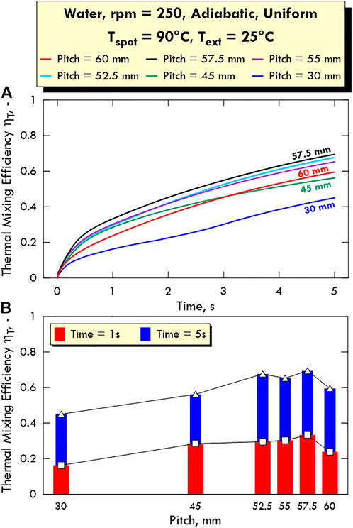
FIGURE 6. Thermal mixing efficiency ${\eta }_T$ (A) as a function of time for different values of pitch and (B) as a function of pitch at 1 and 5 s in adiabatic conditions in uniform configuration. Fluid: water, T_spot = 90°C, T_ext = 25°C.

In fact, looking at the difference between the temperature profiles shown in Figure 5 related to the pitch values of 45 mm and 60 mm at 5 s, we can imagine a priori that there must exist a pitch value for which the extension of the warm zone has a maximum. The investigation at different pitch values is made just in order to evaluate such a maximum.

As a confirmation of our conjecture, the plot in Figure 6A shows that the maximum value of ${\eta }_T$ at 5 s is found at around 57.5 mm, whose corresponding curve is higher than the other ones.

Another interesting aspect to notice is related to the behaviour of the system for pitch values of 45 mm and 60 mm. Indeed, we can observe that, up to around 3 s, η_T is higher for 45 mm, whereas it becomes lower after 3 s. We explain the presence of such a cross by the following considerations.

For a pitch of 45 mm, the spots are closer to each other, this favouring a faster local heating with respect to the 60 mm one due to the lower mass of fluid to heat up. However, a relatively large portion of fluid towards the external wall remains colder due to the high thermal inertia (heat capacity) of water.

Differently, due to the higher angular velocity of the spots and the vicinity to the external wall, which we remind to be not heating, the 60 mm-configuration becomes more effective in heating up a larger amount of more external fluid with a contemporary contribution of the central spot to heat up the colder fluid around the centre. Therefore, a pitch of 60 mm is more effective in heating up the fluid as time passes by.

This situation is depicted better in Figure 6B, where it is possible to observe more clearly not only that the pitch value of 57.5 mm provides the highest value of η_T, but also that the pitch value of 52.5 mm leads to a local maximum at 5 s.

This occurrence states once more the role of the contrasting effect of the distance between two consecutive spots and the vicinity to the wall along with the high thermal inertia of the fluid. To visualise this aspect, we show the temperature profiles at pitch values of 52.5 mm, 55 mm and 57 mm, respectively (Figure 7A).

FIGURE 7

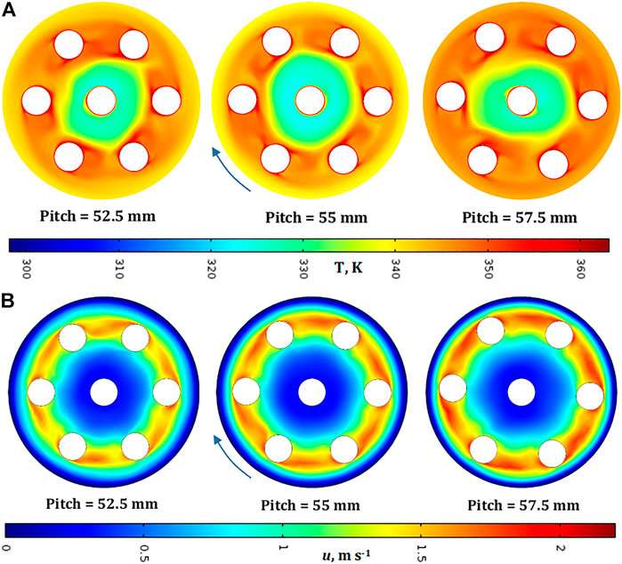
FIGURE 7. (A) Temperature and (B) velocity profiles at 5 s for different pitch values in adiabatic conditions in uniform configuration. Fluid: water, T_spot = 90°C, T_ext = 25°C.

Comparing the profiles at 52.5 mm and 55 mm, it is possible to observe that the former shows a smaller central cold zone along with a slightly warmer zone in the warm crown between consecutive (closer) spots, this leading to the behaviour depicted in Figure 6B.

Figure 7B shows the velocity fields corresponding to the cases shown in. We can observe that the geometrical symmetry reflects also on fluid dynamics, which is characterised by a hotter outer “crown” following the position of the spots in their movement. This also contributes in creating a colder zone around the centre and towards the external perimeter.

5.2.2 Alternate configuration

After identifying the optimal value of pitch for the uniform configuration (57.5 mm), we have investigated the performance shown by the second configuration investigated—i.e., the alternate configuration—by setting the value of the pitch₁ equal to the optimal value of the uniform configuration and varying the second pitch pitch₂ considering the values reported in Table 1 (30 and 40 mm).

As aforementioned, the study of such an additional configuration has arisen from observing that, even for the optimal value of 57.5 mm, the temperature profile of the uniform configuration is characterised by an inner low-temperature ring (Figure 7A). Therefore, we have thought that decreasing the distance between some of the external spots and the central one could have led to a more uniform temperature distribution and, thus, to a higher thermal mixing efficiency.

Figure 8 shows the temperature profiles for water at 5 s in the considered alternate configuration for three different pitch₂ values, the highest of which corresponds to the uniform optimal configuration. We can observe that the reduction of pitch₂ leads to a more uniform temperature distribution. In particular, by looking at the 30-mm case, the inner low-temperature ring has disappeared, with some small cold spots near the vertices of the inner triangle.

FIGURE 8

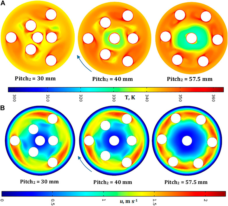
FIGURE 8. (A) Temperature and (B) velocity profiles at 5 s for different pitch₂ values in adiabatic conditions in alternate configuration. Fluid: water, pitch₁ = 57.5 mm, T_spot = 90°C, T_ext = 25°C.

However, the average temperature is lower than the 40-mm case. In practise, at 30 mm, temperature is more uniform but lower than that at 40 mm, this leading to a lower (see later Figure 10A). As for the fluid dynamics of rotation, Figure 8B shows the velocity field for the three values of pitch₂ considered.

As expected, the higher velocity of the outer spots, favouring the convective energy transport with respect to the inner ones, creates a sort of segregation among fluid fillets, augmented by the fluid dynamic inertia of water, which tends to be dragged with a certain delay. Overall, the motion of the fluid fillets becomes integral with the motion of the spots, this leading to the segregated profiles shown in the plots.

5.2.3 Influence of viscosity

To evaluate the optimal thermal performance of the proposed reactor, we have considered also the influence of viscosity increasing artificially the original water viscosity at the same conditions of temperature and pressure by a factor of 100 and 1,000, respectively. The reason for this type of analysis lies in the fact that there are several reactions of interest in which species with a relatively high viscosity, like glycerol (Segur and Oberstar, 1951), can be involved.

Figure 9A shows the temperature profiles with a viscosity augmented by 1,000 times. In this case, the temperature drop with respect to the case at the original viscosity value is significant, but we can observe the common occurrence that the alternate configuration with a pitch₂ value of 40 mm is more performing with respect to the others (see later Figure 10C). The corresponding velocity field is shown in Figure 9B, where we can observe that the colder zones around the centre assume the same qualitative shape as the pitch layout. This occurs because the augmented fluid inertia generates an integral motion difficult to break by the spot shape, this leading to an inefficient heat transmission.

FIGURE 9

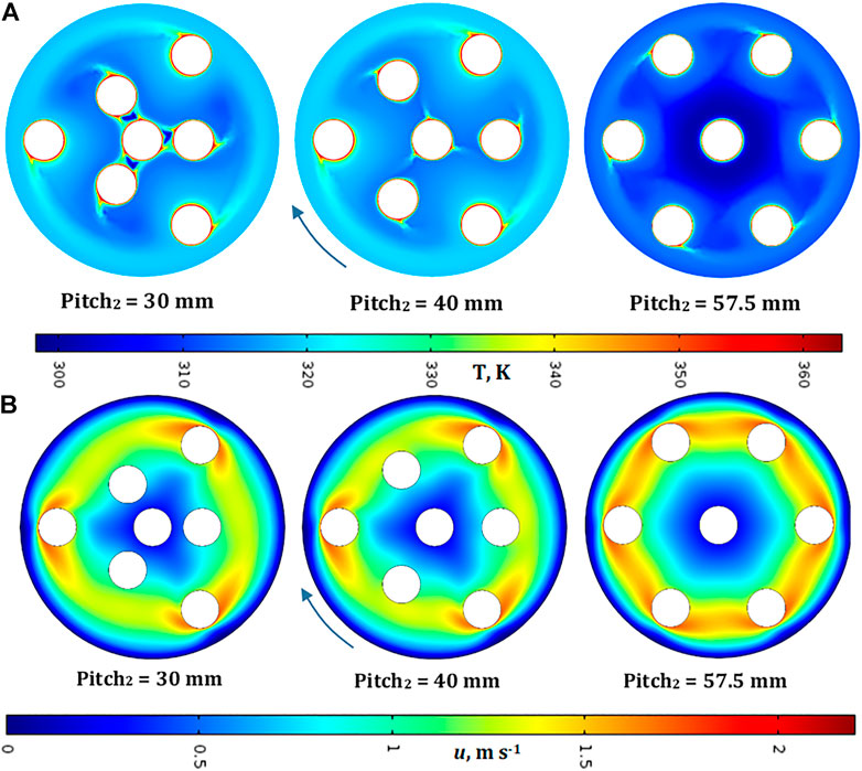
FIGURE 9. (A) Temperature and (B) velocity profiles at 5 s for different pitch₂ values in adiabatic conditionsin alternate configuration. Fluid: water, viscosity = 1,000 μ₀, pitch₁ = 57.5 mm, T_spot = 90°C, T_ext = 25°C.

FIGURE 10

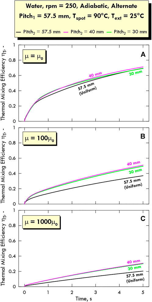
FIGURE 10. Time profile of the thermal mixing efficiency η_T for different values of pitch in alternate configuration at different values of viscosity μ. Fluid: water, T_spot = 90°C, T_ext = 25°C.

Figure 10 summarises the results shown in the previous figures in terms of thermal mixing efficiency. As anticipated above, the configuration with a pitch₂ of 40 mm is the most efficient one in all cases, especially when dealing with highly viscous fluids. An interesting aspect to notice is that the difference of performance between 40 and 30 mm becomes gradually lower as viscosity increases, whilst the difference with the uniform case (57.5 mm) increases at first and slightly decreases towards higher viscosity values. This indicates clearly that the performance of the alternate configuration at relatively high viscosity does not depend much on the secondary pitch provided that the inner spots be not too far from the centre.

Overall, the uniform configuration shows lower performances than the alternate one due to a certain redundancy effect of the spots, each of which tends to heat up the fluid in the same zone already partially covered by another spot.

5.3 Case study 2: Argon gas

To investigate the effect of the thermal inertia, the same simulations carried out for water are performed for argon gas at the same conditions. However, as we already found that the non-adiabatic condition does not influence significantly the behaviour of the system, for argon gas we just consider adiabatic systems.

5.3.1 Uniform configuration

The results related to the uniform configuration at the pitch values of 30 mm, 45 mm and 60 mm are shown in Figure 11A,B in terms of temperature profiles. The first aspect to notice is that the overall mean temperature in the system is higher than that observed for water. This is due to the much lower thermal inertia of the gas, which is heated up much faster than liquid water.

FIGURE 11

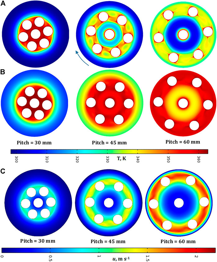
FIGURE 11. Temperature profiles at (A) 1 s and (B) 5 s and (C) velocity profile inadiabatic conditions in uniform configuration. Fluid: argon, T_spot = 90°C, T_ext = 25°C.

Furthermore, the qualitative behaviour of the gas systems at 1 s is similar to the water one in terms of profile symmetry. However, in this case, the symmetry degree still remains relatively high even at 5 s, this being due to the much lower density of the gas implying a much lower momentum transfer among fluid fillets during rotation.

Also in this case, the difference between the profiles at 45 and 60 mm suggests that there must exist a certain pitch at which the extension of the cold zones are minimum, this implying a higher value of thermal mixing efficiency ${\eta }_T$.

Figure 11C shows the corresponding velocity profiles. We can observe again the integral motion of the fluid, even though in this case the fluid fillets are much more mobile due to a much lower viscosity.

To investigate the possible presence of an optimal pitch value, we performed simulations for argon at the same pitch values as those considered for water. The results are shown in Figure 12A in terms of time profiles of η_T and in Figure 12B in terms of ${\eta }_T$ vs. pitch at 1 s and 5 s, respectively.

FIGURE 12

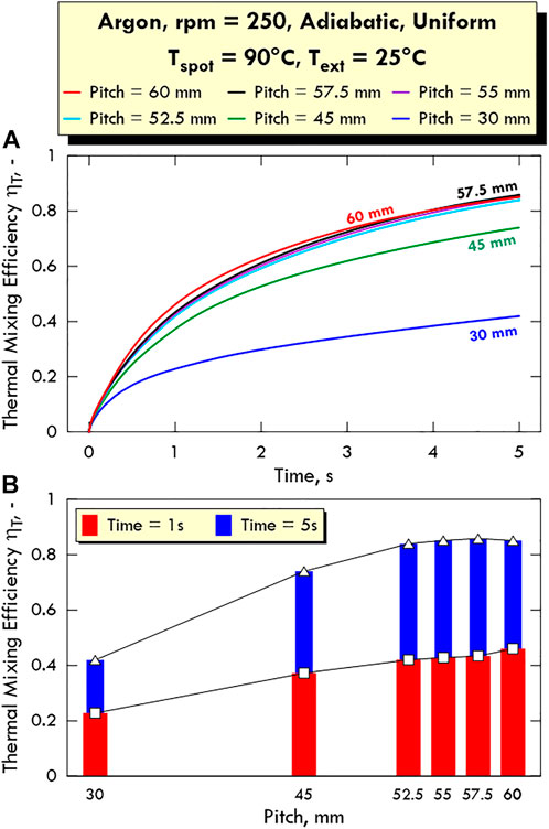
FIGURE 12. Thermal mixing efficiency η_T (A) as a function of time for different values of pitch and (B) as a function of pitch at 1 and 5 s in adiabatic conditions in uniform configuration. Fluid: argon, T_spot = 90°C, T_ext = 25°C.

As for Figure 12A, we can observe that, up to around 3 s, there are no crossing between the ${\eta }_T$ profiles, the highest of which being that at 60 mm. However, as time passes by, the profile at 57.5 mm becomes higher than that at 60 mm. We explain this occurrence with the same considerations made for the case of water, with the difference that, in this second case, the much lower thermal inertia of argon makes the discrepancy among profile much smaller.

This situation can be better represented in Figure 12B, where ${\eta }_T$ is found to increase monotonically with increasing pitch at a time of 1 s, whereas a maximum value is identified around the pitch value of 57.5 mm at 5 s.

As done for water, to understand better the reason for this finding, also in this second case we show the temperature profiles in the system at the three pitch values near the maximum η_T (Figure 13). We can observe that the temperature in the inner zone for a pitch of 55 mm is higher than that for the pitch values of 57.5 mm and 60 mm due to a shorter distance from the central spot. However, for the same reason, the temperature near the external wall is the lowest among the three. On the other side, the temperature in the inner zone for a pitch of 60 mm is the lowest and the temperature near wall is the highest because the spots are closer to the wall. Therefore, the intermediate pitch value of 57.5 mm shows an optimal balance between the other two cases, this resulting in a higher value of ${\eta }_T$.

FIGURE 13

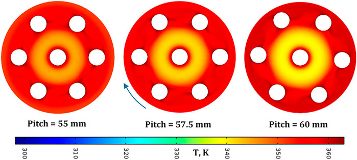
FIGURE 13. Temperature profiles at 5 s for different pitch values in adiabatic conditions in uniform configuration. Fluid: argon, T_spot = 90°C, T_ext = 25°C.

The relevant aspect of the existence of an optimal pitch value around 57.5 mm, corresponding to a pitch/vessel diameter ratio of around 0.36, for two completely different fluids like water and argon gas is a clear demonstration that this result can be somehow generalised, which requires, however, a wider analysis considering other geometrical parameters.

5.3.2 Alternate configuration

Figure 14 shows the temperature profiles obtained for argon in alternate configuration at the same pitch₂ values as those considered for water. The lower thermal inertia of argon makes the heating of the system faster than in the case of water. We can observe that the alternate configuration prevents the formation of a colder zones around the centre, making the temperature distribution more uniform. The profiles shown in Figure 14A lead to the thermal mixing efficiency profiles shown in Figure 14B, from where we can observe that the case at a pitch₂ of 40 mm shows the highest performance amongst the values investigated. Finally, a longer fluid-dynamic simulation performed on pitch₂ of 40 mm revealed that a homogeneous temperature distribution is achieved in almost 13 s.

FIGURE 14

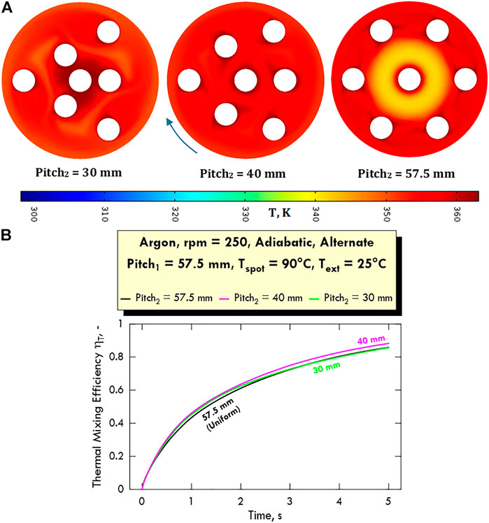
FIGURE 14. (A) Temperature profiles at 5 s and (B) time profile of the thermal mixing efficiency η_T for different pitch₂ values in adiabatic conditions in alternate configuration. Fluid: argon, T_spot = 90°C, T_ext = 25°C.

5.4 Heat transfer coefficient

To give information on the heat transfer efficiency in the system investigated, in Figure 15 we show the time profiles of the overall heat transfer coefficient h_T for water and argon in both uniform (Figure 15A) and alternate configuration (Figure 15B) calculated as reported in Section 3.3 for different pitch values. As shown in the plots, ${\eta }_T$ is observed to averagely increase at higher pitch values. The difference in the order of magnitude between water and argon is caused by the difference in thermal conductivity, which is much higher for the former (around 6 W m⁻² K⁻¹ at room conditions) than the latter (around 0.016 W m⁻² K⁻¹ at room conditions). Furthermore, we can observe that the alternate configuration provides higher h_T values than the uniform one, whose difference among pitch values are more significant than in the alternate configuration.

FIGURE 15

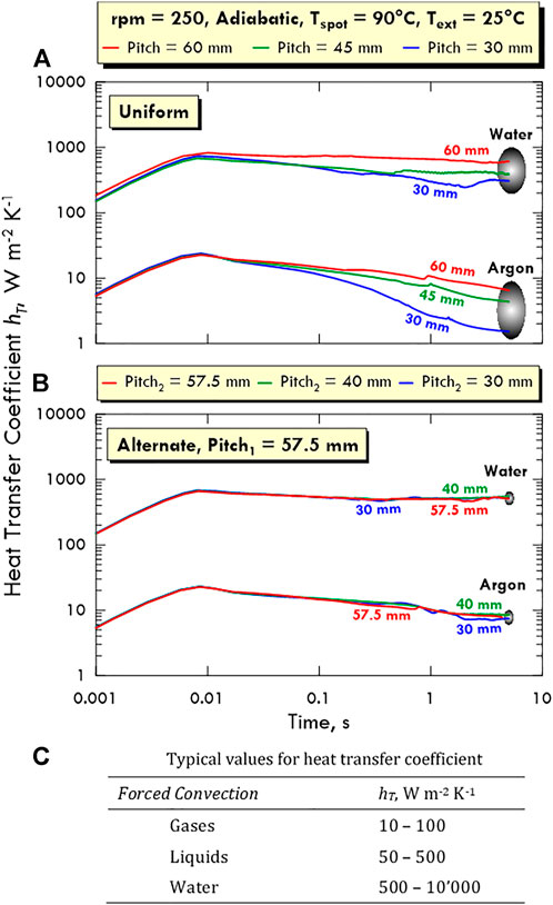
FIGURE 15. Time profile of the heat transfer coefficient h_T for different pitch values for both fluids in (A) uniform and (B) alternate configuration. (C) Typical values of h_T in different cases. Values reported from the Table 14.1-1 of Bird et al. (2002). T_spot = 90°C, T_ext = 25°C.

The values of ${\eta }_T$ calculated from the simulation profiles are compared to some typical data taken from Grober et al. (1955) and reported in the textbook of Bird et al. (2002), some of which are also reported below the plots. As can be observed, the calculated values are perfectly in line with the range indicated in the literature, this confirming the goodness of estimation.

6 Conclusion

In this work, the optimal temperature distribution in the fluid phase inside a novel matrix-in-batch automated rotating patented reactor, namely OnePot^©, was assessed by a computational fluid dynamic (CFD) approach.

The characteristics of this novel reactor provided several advantages in terms of precision of temperature, concentration control and homogeneity. Indeed, the presence of rotating thermal spots allowed a high uniformity degree of the temperature distribution in the fluid domain.

The purpose of the present analysis was to understand, and possibly control, the thermal behaviour of the system, thus reducing the number of prototypes and experiments to be run for design and optimisation purposes. Specifically, for the optimisation purpose, we considered two different configurations, here referred to as uniform and alternate. In both of them, seven thermal spots kept at 90°C rotating with a fixed angular velocity of 250 rpm around a rotation axis coincident with the axis of the spot located at the centre of the vessel.

The uniform distribution shows a single equilateral triangular pitch, whereas the alternate one has a radial layout in which the centres of the spots are the vertices of two alternate equilateral triangles (inner and outer). The latter is characterised by two different values of pitch—namely pitch₁ (larger) and pitch₂ (smaller)—the first of which is set to the fixed value of the optimal pitch identified for the uniform configuration (57.5 mm). The alternate configuration was considered to reduce a certain inefficiency in the temperature distribution present in the uniform configuration.

To conduct this investigation, we performed several CFD simulations in transient and laminar conditions over a 2-D cross-section of the real 3-D system by considering different values of pitches and two different fluids—i.e., liquid water and argon gas. Moreover, we studied also the effect of viscosity by augmenting artificially the viscosity of water by 100 and 1,000 times.

In order to get a quantitative measure of the uniformity degree of the temperature distribution from the calculated 2-D temperature profiles, we introduced a new dimensionless parameter named thermal mixing efficiency ranging within (0, 1), where zero corresponds to the worst case in which the fluid is still at the nominal room temperature (set at 25°C), and the unity corresponds to the best case in which the entire fluid has reached the nominal temperature of the spots.

As a remarkable result, we found that for the uniform configuration, there exists an optimal pitch value (57.5 mm ca.)—corresponding to around 36% of the vessel diameter—for which the thermal mixing efficiency shows a maximum at the highest time value considered (5 s). The significance of this result lies in the fact that we found the same optimal pitch value for both water and argon, this suggesting that such a finding can be generalised to whatever fluid.

As for the alternate configuration, we found that it provides a better temperature distribution in the reactor, especially at high viscosity values. This is because the inner spots are able to counter-balance the effect of the relatively large distance from the centre, preventing in this way the formation of large colder “islands” around the centre.

Moreover, we analysed the time behaviour of the heat transfer coefficients involved in the energy transfer between spot surface and fluid bulk, finding a perfect match with typical values reported in the open literature.

The CFD simulations performed in this work served as a valuable design tool for already-made optimization of the geometric configuration of the spots in this new type of matrix-in-batch reactor, and other types of optimization are going to be carried out for a further development of it. Of particular importance is the analysis of thermal mixing in the tank reactors, which will be focused on reducing the problem of turbulence, which does not allow for a precise control of the homogeneity inside reactor.

Due to the modularity of its configuration, the proposed novel reactor has the potentiality to be used in a number of laboratory-scale as well as industrial applications, especially considering the ease of scalability and of using different three-dimensional layout of matrices.

Data availability statement

The original contributions presented in the study are included in the article/Supplementary Material, further inquiries can be directed to the corresponding authors.

Author contributions

AC and GP performed the computational studies, conceived, and organized the work; MO and MF have invented the technology and designed the reactor structure, as it was patented; SR contributed to realize the reactor integrating the technology. AC and MO were in charge for writing.

Conflict of interest

Author MF was employed by the company B4Chem srl.

The remaining authors declare that the research was conducted in the absence of any commercial or financial relationships that could be construed as a potential conflict of interest.

Publisher’s note

All claims expressed in this article are solely those of the authors and do not necessarily represent those of their affiliated organizations, or those of the publisher, the editors and the reviewers. Any product that may be evaluated in this article, or claim that may be made by its manufacturer, is not guaranteed or endorsed by the publisher.

Supplementary material

The Supplementary Material for this article can be found online at: https://www.frontiersin.org/articles/10.3389/fenrg.2022.964511/full#supplementary-material

References

Balakotaiah, V., and Ratnakar, R. R. (2022). Modular reactors with electrical resistance heating for hydrocarbon cracking and other endothermic reactions. AIChE J. 68, e17542. doi:10.1002/aic.17542

CrossRef Full Text | Google Scholar

Belwal, T., Chemat, F., Venskutonis, P. R., Cravotto, G., Jaiswal, D. K., Bhatt, I. D., et al. (2020). Recent advances in scaling-up of non-conventional extraction techniques: Learning from successes and failures. TrAC Trends Anal. Chem. 127, 115895. doi:10.1016/j.trac.2020.115895

CrossRef Full Text | Google Scholar

Bird, R. B., Stewart, W. E., and Lightfoot, E. N. (2002). Transport phenomena. 2nd Edition. New York (US): John Wiley & Sons. 0-471-41077-2.

Google Scholar

Bran, I., Meric de Bellefon, G., Vairamohan, B., and Yang, J. (2010). Industrial process heating: Current and emerging applications of electrotechnologies. Palo Alto, CA: EPRI, 1020133.

Google Scholar

Caravella, A., Hara, S., Hara, N., Obuchi, A., and Uchisawa, J. (2012). Three-dimensional modeling and simulation of a micrometer-sized particle hierarchical structure with macro- and meso-pores. Chem. Eng. J. 210, 363–373. doi:10.1016/j.cej.2012.08.101

CrossRef Full Text | Google Scholar

Caravella, A., Melone, L., Sun, Y., Brunetti, A., Drioli, E., and Barbieri, G. (2016). Concentration polarization distribution along Pd-based membrane reactors: A modelling approach applied to water-gas shift. Int. J. Hydrogen Energy 41, 2660–2670. doi:10.1016/j.ijhydene.2015.12.141

CrossRef Full Text | Google Scholar

Evrim, C., Chu, X., Silber, F. E., Isaev, A., Weihe, S., and Laurien, E. (2021). Flow features and thermal stress evaluation in turbulent mixing flows. Int. J. Heat. Mass Transf. 178, 121605. doi:10.1016/j.ijheatmasstransfer.2021.121605

CrossRef Full Text | Google Scholar

Francardi, M., and Oliverio, M. (2021). Reattore chimico – N° 102020000008245. Rome: Italian Office of Patents and Trademarks. 16 May 2022. PCT/IB2021/053094. Chemical Reactor. 15 apr 2021.

Google Scholar

Grober, H., Erk, S., and Grigull, U. (1955). Warmeubertragung. 3rd Edition. Berlin: Springer, 158.

Google Scholar

Houlding, T. K., and Rebrov, E. V. (2012). Application of alternative energy forms in catalytic reactor engineering. Green Process Synth. 1, 19–31.

CrossRef Full Text | Google Scholar

Kim, J. K., Son, H. S., and Yun, S. W. (2022). Heat integration of power-to-heat technologies: Case studies on heat recovery systems subject to electrified heating. J. Clean. Prod. 331, 130002. doi:10.1016/j.jclepro.2021.130002

CrossRef Full Text | Google Scholar

Ma, H., Yin, L., Zhou, W., Lv, X., Cao, Y., Shen, X., et al. (2015). Measurement of the temperature and concentration boundary layers from a horizontal rotating cylinder surface. Int. J. Heat. Mass Transf. 87, 481–490. doi:10.1016/j.ijheatmasstransfer.2015.04.035

CrossRef Full Text | Google Scholar

Mandal, B. (2019). Alternate energy sources for sustainable organic synthesis. ChemistrySelect 4, 8301–8310. doi:10.1002/slct.201901653

CrossRef Full Text | Google Scholar

Segur, J. B., and Oberstar, H. E. (1951). Viscosity of glycerol and its aqueous solutions. Ind. Eng. Chem. 43, 2117–2120. doi:10.1021/ie50501a040

CrossRef Full Text | Google Scholar

Siddique, I. J., Salema, A. A., Antunes, E., and Vinu, R. (2022). Technical challenges in scaling up the microwave technology for biomass processing. Renew. Sustain. Energy Rev. 153, 111767. doi:10.1016/j.rser.2021.111767

CrossRef Full Text | Google Scholar

Silla, H. (2003). Chemical process engineering design and economics. Basel: Marcel Dekker.

Google Scholar

Silva, V. L. M., Santos, L. M. N. B. F., and Silva, A. M. S. (2017). Ohmic heating: An emerging concept in organic synthesis. Chem. Eur. J. 23, 7853–7865. doi:10.1002/chem.201700307

PubMed Abstract | CrossRef Full Text | Google Scholar

Son, H. S., Kim, M., and Kim, J. K. (2022). Sustainable process integration of electrification technologies with industrial energy systems. Energy 239, 122060. doi:10.1016/j.energy.2021.122060

CrossRef Full Text | Google Scholar

Turgut, S. S., Karacabey, E., and Küçüköner, E. (2022). A novel system—The simultaneous use of ohmic heating with convective drying: Sensitivity analysis of product quality against process variables. Food bioproc. Tech. 15, 440–458. doi:10.1007/s11947-022-02765-9

CrossRef Full Text | Google Scholar

Zhao, Z., Li, H., Zhao, K., Wang, L., and Gao, X. (2022). Microwave-assisted synthesis of MOFs: Rational design via numerical simulation. Chem. Eng. J. 428, 131006. doi:10.1016/j.cej.2021.131006

CrossRef Full Text | Google Scholar

Nomenclature

Symbol
Description

A Area, m²

C_p Specific heat, J kg⁻¹ K⁻¹

f Rotation frequency, s⁻¹

h_T Heat transfer coefficient, W m⁻² K⁻¹

ID Inner Diameter, m

k Thermal conductivity, W m⁻¹ K⁻¹

L Length, m

n Normal versor,—OD Outer diameter, m

p Pressure, Pa

$\underset{¯}{q}$ Conductive heat flux, W m⁻²

Q,$\dot{Q}$ Heat rate, W

t Time, s

T Temperature

u Velocity field, m s⁻¹

W_p External work rate, W

Greek symbols

a Angular displacement, rad

η_T Thermal mixing efficiency, - μ Viscosity, Pa s

ρ Density, kg m⁻³

ω Angular velocity, rad s⁻¹

Subscripts and superscripts

ext External (vessel or spot temperature)

int Internal (spot temperature)

vess Vessel

Acronyms

CFD Computational Fluid Dynamic(s)

rpm rounds per minute