 Shuo Hu
 Yingzhu Da
 Ailun Wang
- School of Economics, Southwestern University of Finance and Economics, Chengdu, China
As China cannot achieve its emission reduction target without cooperating with other countries, the international carbon trading market has become a part of China’s carbon trading market system. The Belt and Road Initiative (BRI) has brought many development opportunities to countries participating, but critics have also voiced concerns about the environmental and climate degradation it might bring. Thus China is making a great effort towards building a green and low-carbon BRI, part of which is a joint effort with other countries to cut greenhouse gas emission and achieve the 2,030 sustainable development goals. The estimation of abatement costs is the basis of regional carbon emission reduction cooperation and a prerequisite for establishing a regional carbon trading market. Taking into account the technological heterogeneity, this paper uses linear programming to estimate inefficiency level for China and BRI countries, and further calculates the marginal abatement cost (MAC) of carbon dioxide for each country. The results show that after considering technological heterogeneity, the average inefficiency level for China and BRI countries is 2.410%, which is about 26.526% lower than the traditional geographic grouping approach, indicating that the technological heterogeneity among BRI countries is significant and cannot be ignored. Most countries have a low inefficiency level, some countries show a clear trend. China has an average marginal abatement cost of 1440.183 USD/ton. As the marginal abatement cost varies greatly among countries, a large amount of abatement cost could be saved for China and BRI countries if the cost difference is exploited.
1 Introduction
Economic development has always inevitably brought about environmental and climate degradation. The Fifth Assessment Report published by the United Nations Intergovernmental Panel on Climate Change (IPCC) states that almost every region of the world has experienced an increase in temperature, and that the increase in carbon dioxide emissions is the most important cause of this phenomenon (IPCC, 2014). To control the deterioration of the environment, countries around the world have taken various measures. In December 2015, the Paris Agreement was adopted at the Paris Climate Change Conference. The long-term goal of the Paris agreement is to limit the increase in global average temperature to 2°C compared to the pre-industrial period, and to try to limit the temperature increase to 1.5°C. According to a report released by the IPCC, the world’s CO2 emissions would need to be reduced by at least 20 percent of 2010 emissions in 2030 to meet the Paris agreement’s target (Rogelj et al., 2018). As one of the world’s major CO2 emitters (Sun et al., 2019), China has also introduced many policies to encourage the reduction of CO2 emissions, such as limiting the output of heavily polluting enterprises and even closing them (Wang et al., 2021b). In 2020, China first proposed that carbon dioxide emissions should peak by 2030 and work toward carbon neutrality by 2060. In the 2021 session of the National People’s Congress, “carbon peaking” and “carbon neutrality” were also included in the government work report for the first time, reflecting China’s determination to save energy and reduce emissions. As the core policy tool to achieve “carbon peaking” and “carbon neutrality”, China’s carbon emission trading market was launched on 16 July 2021.
However, China cannot achieve its emission reduction target without cooperating with other countries, it requires a joint effort by all countries to achieve the long-term goal set by the Paris Agreement. The international carbon trading market is a part of China’s carbon trading market system. Recently, China set up Hainan International Carbon Emission Trading Center, which will become China’s first carbon market characterized by internationalization and the intersection of domestic and foreign carbon markets. China has issued a variety of policies to promote carbon emission reduction, of which the carbon emission reduction cooperation with the Belt and Road countries is the most important. The Belt and Road Initiative (BRI) formed by the concept of “Silk Road Economic Belt” and “Maritime Silk Road” in 2013 provides an important channel for participating countries to help each other to jointly achieve energy saving and emission reduction goals. Today, China has made significant progress in facilities construction and trade cooperation with the countries covered by the Belt and Road Initiative. However, some critics have point out that the construction of the Belt and Road will on the one hand lead to economic development of the countries involved, but on the other hand, it will also result in greenhouse gas emissions, especially carbon dioxide emissions, being on the rise, which will lead to environmental degradation (Ascensão et al., 2018). Therefore, how to control greenhouse gas emissions while enabling countries along the Belt and Road to achieve their development goals, build a green Belt and Road, and jointly achieve the 2030 sustainable development goals has become an important issue in the process of building the Belt and Road.
Most of the countries covered by the BRI are low to middle-income countries. Figure 1 shows the changes in the share of GDP and energy consumption of the Belt and Road countries from 2006 to 2018. As can be seen in the graph, BRI countries only contribute about 30%–40% of world GDP, but use up to 60% of energy. Both percentages have been rising during this period, but energy consumption rises faster than GDP. This shows that most of the countries involved in the Belt and Road Initiative are still in the stage of rough growth, characterized by high energy use but low output due to inefficient energy use. Most of the countries are trading the environment for their economic growth. Improving the energy efficiency of the Belt and Road countries will make a vital contribution to achieving international environmental protection goals. China, as the initiator of the Belt and Road Initiative, has proposed to support countries to improve energy efficiency and the environment by strengthening communication on ecological and environmental policies and enhancing environmental cooperation mechanisms and platforms. However, improving efficiency and reducing CO2 emissions has a cost, as the technological advances needed to improve efficiency will require investment. And without estimating abatement costs, cooperation in emission reduction among BRI countries would not be possible. The estimation of abatement costs is the basis of regional carbon emission reduction cooperation and a prerequisite for establishing a regional carbon trading market, as it will identify the proper emission target for each country and allow them to trade in the market to minimize their total emission reduction costs.
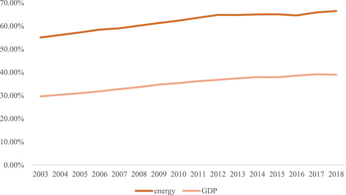
FIGURE 1. BRI countries’ GDP and energy consumption shares.
One important aspect that needs to be taken into account when estimating abatement costs is the economic and technological development levels of the countries in the BRI. The Belt and Road Initiative covers developing countries as well as developed countries, and naturally the economic and technological development levels will be different. Ignoring this difference would be to assume that countries with underdeveloped technologies can reach the production frontier of more developed countries by simply improving efficiency, which is not realistic. If the unbridgeable technological gap is ignored, it will result in an overestimation of inefficiency levels and abatement costs for underdeveloped countries. And therefore, to more accurately estimate abatement costs, it is crucial to consider the technological heterogeneity among BRI countries.
In this context, both for China’s goal of “carbon peaking” and “carbon neutrality,” and for other countries’ goal of sustainable development, it is better to promote inter-regional cooperation in carbon emission reduction than to reduce emissions independently by individual countries. A cross-regional carbon trading market can take advantage of the differences in emission reduction costs among countries along the Belt and Road, thus reducing the costs of emission reduction in each country and enabling each country to achieve sustainable development goals with minimal costs. This paper calculates the marginal abatement cost of each country by taking into account the difference in technological level of each country, and proposes some policy recommendations based on this.
The rest of the paper is organized as follows: Section 2 reviews the literature related to this paper, Section 3 focuses on the methods used in this paper, Section 4 presents the data characteristics, Section 5 discusses the results as well as the implications, and Section 6 concludes with policy recommendations.
2 Literature review
Many methods have been proposed for the measurement of marginal abatement cost, including cost function, model-based methods, distance function and so on. Among them, the distance function method requires only input and output data, which is less demanding than other methods, and therefore has become a more widely used method in recent years [(Zhou et al., 2014; Lee and Zhou, 2015)]. The estimation of marginal abatement costs using distance functions first requires the establishment of a representative energy output function, and the two most commonly used functions are the Shepard distance function and the directional distance function (DDF). The corresponding estimation methods include parametric and non-parametric methods. The non-parametric method, which mainly refers to the data envelopment analysis (DEA) method proposed by Charnes and Cooper (Charnes et al., 1978), does not require the assumption of a specific form of production function, but rather creates a segmented frontier to estimate the production frontier based on the data. Many papers thus choose to combine DDF and DEA to estimate marginal abatement costs [(Boyd et al., 1996), (Battese GE, 2002), (Lee et al., 2002)]. Parametric methods, on the other hand, include two main types: deterministic methods and stochastic frontier analysis (Zhou et al., 2014). For deterministic methods, the linear programming method proposed by Aigner and Chu, 1968 can be used to estimate the parameters in the production function, but the deterministic method does not take into account the random errors in the data. The stochastic frontier analysis method does take into account the random errors, but the production function it yields sometimes fails to satisfy the monotonicity assumption (Zhou et al., 2014). Despite the drawbacks of both methods, they are still very widely used in practice [(Du et al., 2016), (Tang et al., 2016), (Wang et al., 2020)].
However, all the above approaches assume that for all decision-making units (DMU), their optimal production technology is the same, i.e., all decision-making units face the same production frontier. In practice, however, due to differences in infrastructure, education levels, etc. there are often insurmountable technological differences between different decision-making units, which do not decrease over time. The Malmquist-Luenberger productivity index proposed by Oh (Oh, 2010) takes into account the heterogeneity among individuals. Further, Zhang and Choi, 2013 proposed the Meta-frontier Non-radial Malmquist Carbon index (MNMCPI). The above-mentioned applications that take into account heterogeneity are mostly in productivity measurement, and this consideration of heterogeneity is mostly based on geographical location. However, if only geographical location is used as a measure of heterogeneity, it may lead to biased results. Therefore, in Wang et al. (Wang et al., 2021c), three indicators related to the level of economic development were used as the measure of heterogeneity instead of simply grouping by geography, and a program was used to group the DMUs to avoid the possible bias of manual grouping.
As The Belt and Road Initiative rapidly expands in recent years, the amount of literature on energy efficiency and carbon emissions in countries involved in the initiative has gradually increased. Sun et al. (2020) used stochastic frontier method to estimate the persistent and transient energy efficiency of 48 countries along the Belt and Road and found that in general, the persistent energy efficiency of these countries is lower than the transient energy efficiency, indicating that the energy problems of the countries along the Belt and Road are more structural in nature. Qi et al. (2019) measured the total factor energy efficiency (TFEE) of countries along the Belt and Road to examine whether inefficient countries are catching up with efficient countries, and they found that in general, the gap between inefficient countries and efficient countries is closing, and high-income countries are catching up with efficient countries faster. Some literature also explores factors affecting carbon emission amount of BRI countries. Fan et al. (2019) analyzed the changes in CO2 emissions and the drivers behind the changes in 46 countries along the Belt and Road. They found that economic development and potential carbon emissions associated with energy consumption were the most important factors influencing the growth of CO2 emissions, while changes in emission reduction technology and potential emissions were the two most important inhibiting factors. You et al. (2022) analyzed the interaction effects of income inequality and democracy on CO2 emissions, and found that there is an inverted “U” shaped relationship between income equality and CO2 emissions, and that the degree of democracy facilitates this relationship between income equality and CO2 emissions, with high income inequality combined with poor democracy leading to higher CO2 emissions in a country when all else is equal. Muhammad et al. (2020) explored the relationship between urbanization and international trade on CO2 emissions in the BRI countries. The empirical results show that urbanization has an inverted “U” relationship with CO2 emissions only in high-income countries. In addition, FDI increases CO2 emissions, which supports the “pollution paradise” hypothesis.
However, most of the aforementioned literature does not consider the heterogeneity among countries. Therefore, the contribution of this paper can be summarized as follows: first of all, this paper introduces factors measuring national economic environment differences into the calculation of efficiency, mainly foreign direct investment (FDI), trade openness, government expenditure, and institutional quality. FDI can improve the technological level of the host country by bringing advanced technology and skilled workers into the country (Fassio et al., 2019). Meanwhile, the inflow of foreign investment can ease the financial constraints of innovative activities in the host country, ultimately leading to the improvement of technology (Chen et al., 2017). The higher trade openness is, the bigger the market is for enterprises, thus the more incentive there is for the enterprises to innovate (GM Grossman, 1994). Government expenditure could act as an important driver in managing pollution levels (Li et al., 2021). Besides, government expenditure spent on science and technology could encourage the advancement of technology, which ultimately could lead to improvement in efficiency and decrease in emissions (Iqbal et al., 2021). And finally, higher institutional quality leads to better interaction between authorities and firms, resulting in less risk of technological expropriation and other undesired outcomes for firms, and ultimately encourages innovation (Egan, 2013). Adding factors measuring national economic environment differences will make the estimation of production frontier more accurate, and the estimated efficiency will be more accurate compared to models not considering the differences. Moreover, few previous literatures have calculated marginal abatement cost on the country level, and this paper further calculates the marginal abatement cost for each country based on the estimated efficiency, thus providing some reference for BRI countries on how to mitigate total abatement cost while maintaining the amount of emission reduction. This paper has a new contribution in method. Previous literatures used discrete variables to classify production technologies, such as geographic location, whether it is an environmentally friendly city, etc., but did not use continuous variables to classify production technologies. In addition, the method in this paper is different from the clustering method. The clustering method can only group the production technology level according to the Euclidean distance (or other distance function) between the exogenous technical variables, and cannot use the directional distance function and the exogenous technology at the same time. The information about the variable is grouped.
3 Models
3.1 Production technology
All the models in this paper are based on the models proposed in Wang et al. (2021c). First is the modelling of production technologies. Assume that there are K producers in the economy, producer k (k = 1,2,…,K) uses
The output set must satisfy the following assumptions:
The null-jointness assumption ensures the inevitability of undesirable outputs in the production process, no production activities can be carried out without producing undesirable outputs. And weak disposability suggests that when the amount of the desirable output is constant or increasing, the amount of the undesirable output cannot be reduced, meaning that there is a cost to reducing the undesirable output.
Production technology is modeled using the output DDF in this paper. Setting
Where
3.2 Estimating energy environmental efficiency and CO2 marginal abatement cost
After satisfying the above assumptions, this paper follows Färe et al. (2005), and uses the linear programming method proposed by Aigner and Chu, 1968 to estimate the parameters of the DDF.
Assume that every country uses three inputs: capital (
Where
The objective of this linear programming is to minimize the distance between each DMU observation and its production frontier subject to the production technology constraint of Eq. 2. Constraint 1) ensures that each observation is within boundary. Constraints 2) and 3) ensure the non-increasing property of desirable output and the non-decreasing property of undesirable output. The parameter restriction in constraint 4) assigns the translation property to the directional vector. And constraint 5) limits the symmetry property of the model. Eq. 5 can be used to estimate the energy environment inefficiency of each country.
Based on the estimated energy environment inefficiency, CO2 MAC of each country can be calculated using the following equation:
where p is the market price of desirable output, and
3.3 Modeling with economic proximity
And finally, this paper incorporates the economic environment of each country into the production technology to solve the heterogeneity problem. The effect of the environment is determined through multidimensional variables representing economic proximity. This paper selects four representative variables to measure economic proximity, which are FDI, trade openness, government expenditure, and institutional quality. These variables are represented by
The first step is to determine the nearest neighbors of each country. The nearest neighbors are defined as the η provinces with the smallest square of Euclidean distance from the reference province calculated according to environmental variables. The larger the year, the greater the weight given. Therefore, the weighted Euclidean distance square of each country k with respect to other countries m during the sample period can be calculated as:
Where t = 1, 2, …, T represents the sample year.
After ranking the nearest neighbors for each country, the following criteria is used to determine the optimal number of nearest neighbors for country k (represented by
First of all, the optimal number of nearest neighbors should satisfy the null-jointness hypothesis. Specifically, for each country in each period of observation, null-jointness hypothesis is satisfied when
Second, shadow prices are generally considered to be non-negative, thus samples with negative estimated shadow prices are often removed [(Färe et al., 2005); (Ji and Zhou, 2020)]. As can be seen in Eq. 6, shadow price is connected to the monotonicity of both desirable and undesirable outputs, therefore, samples with negative shadow prices do not fit the production technology defined before. The share of non-negative shadow prices is denoted as
Combining the above two constraints, the optimal number of nearest neighbors of reference country k is defined as the
4 Data
The paper uses data of 115 countries along the BRI, including China, from 2006 to 2018. The majority of previous researches select 50 to 60 countries to study. However, as the BRI expands, the number of countries participating is increasing, thus a more accurate production frontier can be estimated by using data of more countries, in turn the estimation of MAC will be more accurate. In addition, since developed countries such as Germany and UK opened the China Railway Express with China after 2011, and the China Railway Express is an important part of the BRI, we will also include the countries that have opened the China Railway Express in the sample. Some researchers have pointed out that the development of BRI countries vary greatly, for example Zhang et al. (2020) divided BRI countries into 5 groups, and discovered significant differences of CO2 emissions and GDP among groups. Thus, for comparison purposes, the countries are divided into 5 groups according to the continent they are in. Countries used and the groups are shown in Table 1.
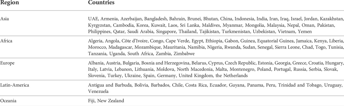
TABLE 1. BRI Country lists.
Three inputs are considered in this paper: capital, labor, and energy. Capital and labor are generally considered to be essential inputs of production, and the addition of energy is because the usage of energy during production is the main reason of the production of undesirable outputs. Capital stock of each country as well as labor data come from the Penn World Table, and the consumption of energy of each country comes from the U.S. Energy Information Administration (EIA).
Two kinds of outputs from production activities are considered. One is desirable output, which is the product that the enterprise wants to produce by engaging in production activities, measured by GDP. The other one is undesirable output, which is environmentally harmful outputs that are inevitable when a company produces desirable output, which is CO2. GDP data comes from the Penn World Table, while CO2 emission data comes from EDGAR (Emissions Database for Global Atmospheric Research).
And finally, as mentioned before, this paper covers 115 countries from 5 different continents who have varying levels of development, and in turn varying levels of production technology. Thus indicators are needed when determining production frontier of each country to identify countries with similar level of development to the reference country, allowing for a more accurate estimation of the production frontier than traditional methods. This paper chooses four indicators: foreign direct investment, total imports and exports, total government spending, and a composite measure of institutional quality. FDI reflects a country’s attractiveness to foreign investment. FDI inflows can directly promote technological progress in the host country through technology spillover effects, while FDI inflows can also increase the capital available to enterprises and indirectly promote technological progress in the host country. Total imports and exports is used as a proxy of a country’s openness (Wang et al., 2021a), the more open a country is, the bigger the market is, and the greater the incentive for firms to innovate. Government expenditure spent on science and technology could promote innovation. Finally, institutional quality is measured from six aspects: voice and accountability, political stability and absence of violence/terrorism, government effectiveness, regulatory quality, rule of law, and control of corruption. Generally speaking, the higher a country’s institutional quality is, the more the government promotes development of the private sector, and the better the protection of intellectual property is, resulting in more incentive for enterprises to innovate. Data on FDI, import and export, and government expenditure comes from the World Development Index, score of institutional quality comes from WGI (The Worldwide Governance Indicators), which covers six aspects as outlined before, with a score between –2.5 and 2.5 for each aspect. This paper takes the average of the scores as a composite measure of institutional quality. Table 2 details the statistical characteristics of the variables, and the statistical characteristics based on geographical subdivisions is shown in Supplementary Datasheet S1.
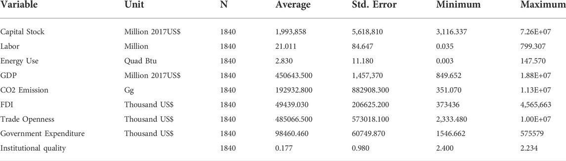
TABLE 2. Summary statistics of the variables.
As can be spotted from the statistical characteristics, variables such as GDP and capital stock vary greatly among regions. Oceania possesses the lowest average of capital stock, labor, and energy use, with the averages being 7.656%, 2.720%, and 8.215% of the highest averages respectively. Asia possesses the highest average in labor and energy use. As most Asian countries are developing countries, production technology is relatively underdeveloped, thus they tend to use more energy when producing. The regional differences in the three inputs are considerably big and therefore cannot be ignored in the calculation of marginal abatement costs. The two outputs are similar to the inputs. Oceania possesses the lowest average GDP, which is 10.622% of the highest average possessed by Asia. CO2 emissions exhibit a similar pattern, with a vast difference between the lowest average and the highest. It follows that there is a gap in production technology between regions, and that this gap does not decrease over time. If the efficiency is estimated using the normal DDF without taking into account the technology gap, the efficiency of the less developed countries will be lower than the real value because it includes the technology gap that cannot be eliminated. Therefore, it is necessary to include variables that measure the economic environment of different countries to ensure the accuracy of the estimates of efficiency and shadow prices.
5 Empirical results
5.1 Nearest neighbors
Table 3 shows the number of nearest neighbors for all countries. Due to the number of countries involved, the paper will not give a detailed list of all the nearest neighbors selected for each reference country. The nearest neighbors chosen for every country differ significantly from the results from geographic division. For example, among the nearest neighbors of Azerbaijan there are many countries that are not in Asia but have a similar level of development, such as Fiji, Togo, etc. For European countries such as Poland, other countries in Europe are mostly chosen as nearest neighbors, but among its nearest neighbors there are also countries that are not in Europe but are also more developed, such as Qatar. It can also be noted that only one country has a number of nearest neighbors equal to the number of countries remaining after removing it, which is 114. This result also confirms the previous hypothesis that there are differences in the technological levels of countries at different levels of development, and this gap is significant for most countries. If this unbridgeable gap is not taken into account, then the final measured efficiency levels and marginal abatement costs of countries will also be biased.
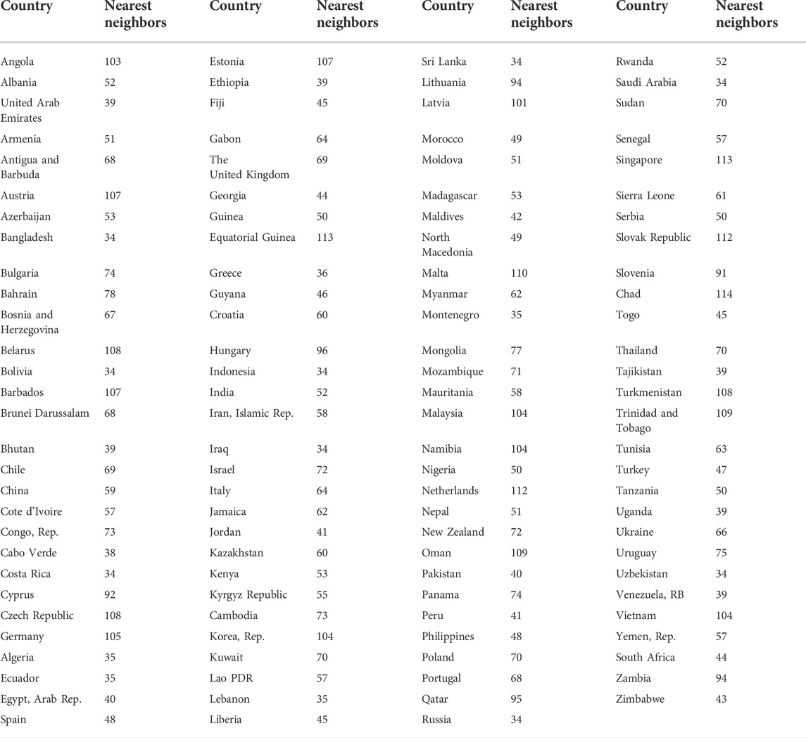
TABLE 3. The number of nearest neighbors.
5.2 Estimation of environmental inefficiency
After determining nearest neighbors of each country, this paper proceeds to estimate the environmental inefficiency of every country using Eqs 4, 5. The estimated energy environmental inefficiency for each country is presented in Supplementary Datasheet S1, the time trend for each country is shown in Figure 2, and the time trend of average inefficiency level is shown in Figure 3. Several conclusions can be drawn from the result: first of all, the average inefficiency of the whole sample is 2.410%, which indicates an efficiency loss of 2.410% for BRI countries. The average efficiency loss remained below or slightly higher than the average except for 2006, 2009, and 2018. Second, among the 115 countries, Russia displays a significant downward trend of inefficiency. After hitting a peak in 2009, Russia has been improving its energy efficiency since. Russia’s economy is one of the most energy-intensive ones among the industrialized countries, fuel and energy sector is one of the biggest sectors in the country (Lobova et al., 2019). Russia was identified by the International Energy Agency (IEA) in 2011 as having very high energy saving potential, as is evident in our result since Russia reached an inefficiency level of more than 50% in 2009. Since then, several state policies have been introduced to increase efficiency, such as the “energy efficiency and energy development” program, technological regulations, etc. (Lobova et al., 2019) The implementation of relevant policies has seen some result, but in 2018 the inefficiency level of Russia was still at 16.697%, significantly higher than the majority of countries covered, meaning that existing mechanisms do not fully exploit the energy saving potential that Russia has, consistent with existing literature [(Lobova et al., 2019), (Strielkowski et al., 2021)]. Thus more work still needs to be done by Russian authorities to reach full energy saving potential.
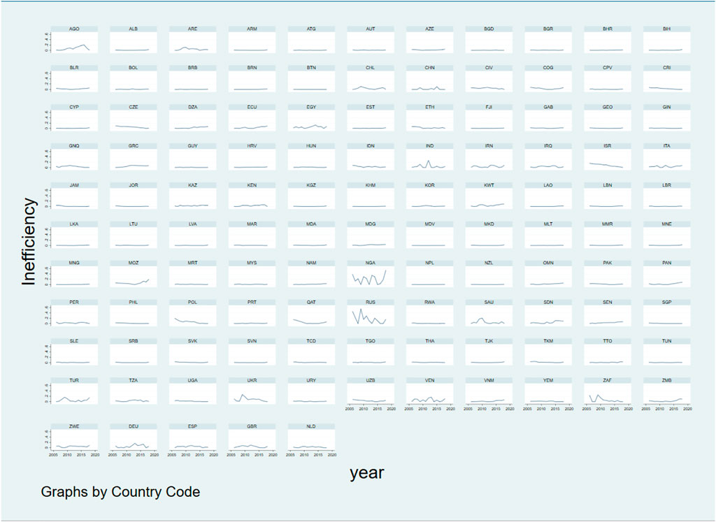
FIGURE 2. Time trend of inefficiency for each BRI country.
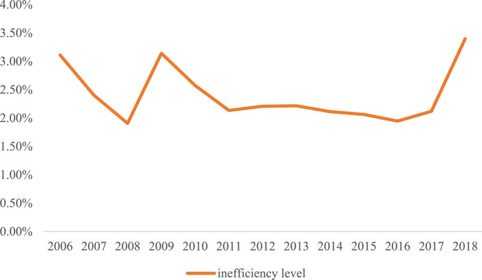
FIGURE 3. Average inefficiency level of China and BRI countries.
The majority of countries’ inefficiency averages are below the total sample mean, the lowest of which is Maldives with an average inefficiency of only 0.063%. It can also be seen from the estimation results that the inefficiency value of Maldives has basically remained around 0 during the sample time period, which shows that Maldives has basically been producing on its production frontier. There are 42 countries above the mean value of the total sample, the highest of which is Nigeria with 20.517%. The inefficiency level of Nigeria has fluctuated significantly during the sample period, but remained at around 30% for most of the sample period. This implies that the authority needs to do more to achieve sustainable development, and they have to ensure that the policies implemented have a consistent effect on the energy efficiency.
Finally, we divided the sample countries into 5 groups according to the continent on which the country is located (Table 1). Assume that these countries have the same technological frontier and use Eq. 4 to calculate the inefficiency. Figure 4 gives a comparison of inefficiency estimates from two approaches: the proposed approach in this paper and the approach with geographic grouping. The average inefficiency level of geographic grouping approach is 3.280%, whereas the average inefficiency level of the proposed approach is only 2.410%. As can be seen in the graph, estimates with geographic grouping is consistently higher than estimates in this paper, proving again that the technological heterogeneity among BRI countries cannot be measured simply by geographic location, and ignoring it will result in overestimation of inefficiency levels.
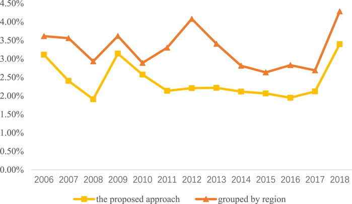
FIGURE 4. Inefficiency levels calculated by different approaches.
5.3 Estimation the marginal abatement cost of CO2
Finally, based on the above estimated inefficiency level, this paper estimates the CO2 MAC of each country using Eq. 6. The average MAC of each country is shown in Supplementary Datasheet S1, units are in USD per ton. The average MAC of the entire sample is 6,274.722 USD/ton. As can be seen in the result, Ethiopia possesses the highest average MAC of 4,9401.200 USD/ton. The average MAC of only 27 countries is above 10,000 USD/ton, and the country with the lowest average MAC is South Africa, with an average of only 224.127 USD/ton. It can be seen from the result that the cost of emission reduction varies greatly from country to country, so if carbon trading can be achieved between countries, it will be possible to minimize the total cost while maximizing the amount of emission reduction. Figure 5 illustrates the average marginal abatement cost and its growth rate for each year from 2006 to 2018. As can be seen in the graph, the growth rate has remained relatively close to 0 during the sample period except for 2009 and 2010.
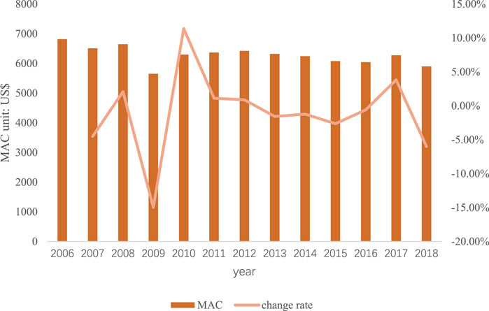
FIGURE 5. Average marginal abatement cost and growth rate.
Among the 115 countries, China ranks 53, with an average MAC of 1440.183 USD/ton. Many countries whose average MAC are lower are underdeveloped countries, such as Pakistan, Moldova, Costa Rica, etc. On average, the MAC in these countries is 342.040 USD/ton lower than in China. If China-BRI international trade market can be set up, a large saving in abatement costs could be achieved.
6 Conclusion
As China cannot achieve its emission reduction target without cooperating with other countries, the international carbon trading market is a part of China’s carbon trading market system. The estimation of abatement costs is the basis of regional carbon emission reduction cooperation and a prerequisite for establishing a regional carbon emission market. Most of the previous literature does not take into account the heterogeneity of production technologies when measuring the environmental efficiency for China and BRI countries. Therefore, this paper estimates the energy efficiency and the marginal abatement cost of CO2 in China and BRI countries while considering the heterogeneity of production technologies.
The conclusions are as follows: First, FDI, trade openness, government expenditure, and institutional quality are selected to measure economic proximity. And, the selection of nearest neighbors shows that there are indeed unbridgeable technological differences between countries, and such unbridgeable differences should be excluded from the efficiency measurement. Second, the average inefficiency of the countries along the Belt and Road is 2.410%. Although the inefficiency of most countries is low and does not change significantly during the sample time, some countries show a clear trend. The average inefficiency level of the proposed approach is about 26.526% lower than the traditional geographic grouping approach, indicating that the technological heterogeneity among BRI countries is significant and cannot be ignored. Finally, the marginal abatement costs of the countries along the Belt and Road show a large difference. China ranks 53, with an average MAC of 1440.183 USD/ton. If China- BRI international trade market can be set up, a large saving in abatement costs could be achieved.
One of the goals of the Belt and Road Initiative is to construct a green BRI and jointly achieve the 2030 Sustainable Development Goals. But emissions reduction, a hot topic that has been mentioned repeatedly in recent years, is not the same for every country. Therefore, China, as the initiator of the Belt and Road Initiative, should not only lead by example, but also help other countries to achieve the goal of energy saving and emission reduction. The analysis in this paper can, on the one hand, help the Chinese government identify the countries most in need of help, and thus help solve their problems through policy assistance, facility construction, etc. On the other hand, it can also identify the differences in the difficulty of emission reduction among countries, so as to help them achieve their own emission reduction goals within their capacity, and to minimize the total cost of emission reduction while maximizing the amount of emission reduction. The analysis in this paper includes only carbon dioxide due to data limitations, but the greenhouse gases produced by energy use include not only carbon dioxide, but also sulfur dioxide, nitrogen oxides, and so on. The reduction of carbon dioxide emissions often affects the emissions of other pollutants as well. Therefore, if other pollutants are also taken into account, the marginal abatement cost of carbon dioxide can be estimated more accurately.
Data availability statement
The original contributions presented in the study are included in the article/Supplementary Material, further inquiries can be directed to the corresponding author.
Author contributions
SH: conceptualization, investigation, experiment design and data analytical methods, funding acquisition, project administration, methodology. YD: investigation, experiment design and data analytical methods, coding, writing. AW: conceptualization, Investigation, Experiment design and data analytical methods, funding acquisition, project administration, methodology, Writing—review and editing.
Funding
This study is supported by National Natural Science Foundation of China (Grant Number 72004185), Fundamental Research Funds for the Central Universities (Grant Number JBK2202009) and Chengdu Philosophy and Social Sciences Planning Project (Grant Number 2022C10).
Conflict of interest
The authors declare that the research was conducted in the absence of any commercial or financial relationships that could be construed as a potential conflict of interest.
Publisher’s note
All claims expressed in this article are solely those of the authors and do not necessarily represent those of their affiliated organizations, or those of the publisher, the editors and the reviewers. Any product that may be evaluated in this article, or claim that may be made by its manufacturer, is not guaranteed or endorsed by the publisher.
Supplementary material
The Supplementary Material for this article can be found online at: https://www.frontiersin.org/articles/10.3389/fenrg.2022.957071/full#supplementary-material
References
Aigner, D. J., and Chu, S. F. (1968). On estimating the industry production function. Am. Econ. Rev. 58, 826–839.
Ascensão, F., Fahrig, L., Clevenger, A. P., Corlett, R. T., Jaeger, J. A. G., Laurance, W. F., et al. (2018). Environmental challenges for the belt and road initiative. Nat. Sustain. 1, 206–209. doi:10.1038/s41893-018-0059-3
Battese Ge, R. D. (2002). Technology gap, efficiency, and a stochastic metafrontier function. Int. J. Bus. Econ., 87–93.
Boyd, G., Molburg, J., and Prince, R. (1996). Alternative methods of marginal abatement cost estimation: Non- parametric distance functions. United States: Decision and Information Sciences Div. Argonne National Lab., IL.
Charnes, A., Cooper, W. W., and Rhodes, E. (1978). Measuring the efficiency of decision making units. Eur. J. Operational Res. 2, 429–444. doi:10.1016/0377-2217(78)90138-8
Chen, Y., Hua, X., and Boateng, A. (2017). Effects of foreign acquisitions on financial constraints, productivity and investment in R&D of target firms in China. Int. Bus. Rev. 26, 640–651. doi:10.1016/j.ibusrev.2016.12.005
Du, L., Hanley, A., and Zhang, N. (2016). Environmental technical efficiency, technology gap and shadow price of coal-fuelled power plants in China: A parametric meta-frontier analysis. Resour. Energy Econ. 43, 14–32. doi:10.1016/j.reseneeco.2015.11.001
Egan, P. J. W. (2013). R& D in the periphery? Foreign direct investment, innovation, and institutional quality in developing countries. Bus. Polit. 15, 1–32. doi:10.1515/bap-2012-0038
Fan, J.-L., Da, Y.-B., Wan, S.-L., Zhang, M., Cao, Z., Wang, Y., et al. (2019). Determinants of carbon emissions in ‘belt and road initiative’ countries: A production technology perspective. Appl. Energy 239, 268–279. doi:10.1016/j.apenergy.2019.01.201
Färe, R., Grosskopf, S., Noh, D.-W., and Weber, W. (2005). Characteristics of a polluting technology: Theory and practice. J. Econ. 126, 469–492. doi:10.1016/j.jeconom.2004.05.010
Fassio, C., Montobbio, F., and Venturini, A. (2019). Skilled migration and innovation in European industries. Res. Policy 48, 706–718. doi:10.1016/j.respol.2018.11.002
Gm Grossman, E. H., and Helpman, E. (1994). Endogenous innovation in the theory of growth. J. Econ. Perspect. 8, 23–44. doi:10.1257/jep.8.1.23
IPCC (2014). Climate change 2014: Synthesis report. Contribution of working groups I, II and III to the fifth assessment report of the intergovernmental panel on climate change. Editors Core Writing TeamR. K. Pachauri, and L. A. Meyer (Geneva, Switzerland: IPCC), 151.
Iqbal, S., Taghizadeh-Hesary, F., Mohsin, M., and Iqbal, W. J. E., (2021). Assessing the role of the green finance index in environmental pollution reduction. 39, 12, doi:10.25115/eea.v39i3.4140
Ji, D. J., and Zhou, P. (2020). Marginal abatement cost, air pollution and economic growth: Evidence from Chinese cities. Energy Econ. 86, 104658. doi:10.1016/j.eneco.2019.104658
Lee, C.-Y., and Zhou, P. (2015). Directional shadow price estimation of CO2, SO2 and NOx in the United States coal power industry 1990–2010. Energy Econ. 51, 493–502. doi:10.1016/j.eneco.2015.08.010
Lee, J.-D., Park, J.-B., and Kim, T.-Y. (2002). Estimation of the shadow prices of pollutants with production/environment inefficiency taken into account: A nonparametric directional distance function approach. J. Environ. Manag. 64, 365–375. doi:10.1006/jema.2001.0480
Li, Z., Wang, J., and Che, S. (2021). Synergistic effect of carbon trading scheme on carbon dioxide and atmospheric pollutants. Sustainability 13, 5403. doi:10.3390/su13105403
Lobova, S., Bogoviz, A., Ragulina, Y., and Alekseev, A. (2019). The fuel and energy complex of Russia: Analyzing energy efficiency policies at the federal level. Int. J. Energy Econ. Policy 9, 205–211.
Muhammad, S., Long, X., Salman, M., and Dauda, L. (2020). Effect of urbanization and international trade on CO2 emissions across 65 belt and road initiative countries. Energy 196, 117102. doi:10.1016/j.energy.2020.117102
Oh, D.-h. (2010). A metafrontier approach for measuring an environmentally sensitive productivity growth index. Energy Econ. 32, 146–157. doi:10.1016/j.eneco.2009.07.006
Qi, S., Peng, H., Zhang, X., and Tan, X. (2019). Is energy efficiency of belt and road initiative countries catching up or falling behind? Evidence from a panel quantile regression approach. Appl. Energy 253, 113581. doi:10.1016/j.apenergy.2019.113581
Rogelj, J., Shindell, D., Jiang, K., Fifita, S., Forster, P., Ginzburg, V., et al. (2018). “Global Warming of 1.5°C. An IPCC Special Report on the impacts of global warming of 1.5°C above pre-industrial levels and related global greenhouse gas emission pathways,” in The context of strengthening the global response to the threat of climate change, sustainable development, and efforts to eradicate poverty.
Strielkowski, W., Sherstobitova, A., Rovny, P., and Evteeva, T. (2021). Increasing energy efficiency and modernization of energy systems in Russia: A review. Energies (Basel). 14, 3164. doi:10.3390/en14113164
Sun, C., Li, Z., Ma, T., and He, R. (2019). Carbon efficiency and international specialization position: Evidence from global value chain position index of manufacture. Energy Policy 128, 235–242. doi:10.1016/j.enpol.2018.12.058
Sun, H., Edziah, B. K., Song, X., Kporsu, A. K., and Taghizadeh-Hesary, F. (2020). Estimating persistent and transient energy efficiency in belt and road countries: A stochastic frontier analysis. Energies 13, 3837. doi:10.3390/en13153837
Tang, K., Gong, C., and Wang, D. (2016). Reduction potential, shadow prices, and pollution costs of agricultural pollutants in China. Sci. Total Environ. 541, 42–50. doi:10.1016/j.scitotenv.2015.09.013
Wang, A., Hu, S., and Li, J. (2021a). Does economic development help achieve the goals of environmental regulation? Evidence from partially linear functional-coefficient model. Energy Econ. 103, 105618. doi:10.1016/j.eneco.2021.105618
Wang, A., Hu, S., and Lin, B. (2021b). Can environmental regulation solve pollution problems? Theoretical model and empirical research based on the skill premium. Energy Econ. 94, 105068. doi:10.1016/j.eneco.2020.105068
Wang, A., Hu, S., and Lin, B. (2021c). Emission abatement cost in China with consideration of technological heterogeneity. Appl. Energy 290, 116748. doi:10.1016/j.apenergy.2021.116748
Wang, Z., Chen, H., Huo, R., Wang, B., and Zhang, B. (2020). Marginal abatement cost under the constraint of carbon emission reduction targets: An empirical analysis for different regions in China. J. Clean. Prod. 249, 119362. doi:10.1016/j.jclepro.2019.119362
You, W., Li, Y., Guo, P., and Guo, Y. (2020). Income inequality and CO2 emissions in belt and road initiative countries: The role of democracy. Environ. Sci. Pollut. Res. 27, 6278–6299. doi:10.1007/s11356-019-07242-z
Zhang, N., and Choi, Y. (2013). Total-factor carbon emission performance of fossil fuel power plants in China: A metafrontier non-radial malmquist index analysis. Energy Econ. 40, 549–559. doi:10.1016/j.eneco.2013.08.012
Zhang, Y.-J., Jin, Y.-L., and Shen, B. (2020). Measuring the energy saving and CO2 emissions reduction potential under China’s belt and road initiative. Comput. Econ. 55, 1095–1116. doi:10.1007/s10614-018-9839-0
Zhou, P., Zhou, X., and Fan, L. W. (2014). On estimating shadow prices of undesirable outputs with efficiency models: A literature review. Appl. Energy 130, 799–806. doi:10.1016/j.apenergy.2014.02.049
Keywords: CO2 abatement cost, Belt and Road Initiative, technological heterogeneity, marginal abatement cost, economic proximity
Citation: Hu S, Da Y and Wang A (2022) CO2 abatement costs in China and BRI countries: From the perspective of technological heterogeneity. Front. Energy Res. 10:957071. doi: 10.3389/fenrg.2022.957071
Received: 30 May 2022; Accepted: 18 July 2022;
Published: 22 August 2022.
Edited by:
Xin Yao, Xiamen University, ChinaReviewed by:
Zhenni Chen, Xi’an Jiaotong University, ChinaGang Du, East China Normal University, China
Ping Zhang, Wuhan University, China
Copyright © 2022 Hu, Da and Wang. This is an open-access article distributed under the terms of the Creative Commons Attribution License (CC BY). The use, distribution or reproduction in other forums is permitted, provided the original author(s) and the copyright owner(s) are credited and that the original publication in this journal is cited, in accordance with accepted academic practice. No use, distribution or reproduction is permitted which does not comply with these terms.
*Correspondence: Ailun Wang, d2FuZ2FsQHN3dWZlLmVkdS5jbg==