A prediction on the impacts of China’s national emissions trading scheme on CO2 emissions from electricity generation

One of the government policies that can reduce CO₂ emissions is the Emissions Trading Scheme (ETS), which was implemented in the Chinese economy on 16 July 2021. It is the largest ETS in the world, covering 12% of global CO₂ emissions. Since this policy has not been experienced in China, it is necessary to predict its impact on CO₂ emissions in this country. Furthermore, electricity and heat production is the major contributor to total CO₂ emissions from fuel combustion. Therefore, this study attempts to predict the impact of the emissions trading scheme on CO₂ emissions from the combustion of coal, oil and natural gas in electricity generation using annual data from 1985 to 2019. For this purpose, this study first predicts CO₂ emissions from the combustion of coal, oil and natural gas for electricity generation in power plants using ARIMA and structural Vector Autoregression (SVAR) techniques over the 2020–2030 period. It then estimates the short- and long-run impact of the ETS policy on CO₂ emissions from the combustion of coal, oil and natural gas in power plants over the projected period (2020–2030) by employing the ARDL methodology. The results suggest that the ETS policy is effective in reducing the CO₂ emissions from the combustion of all fuels in electricity generation over the long-run. This is because of the increase in CO₂ emissions from the combustion of these fuels in power plants in the long run, which exceed the threshold value. But in the short-run, it has a negative and statistically significant impact only on CO₂ emissions from the natural gas power plants. These results suggest that improving the efficiency of all fuels can significantly reduce CO₂ emissions in electricity generation from coal, oil and natural gas in the short- and long-run. They also enable China’s energy policymakers to update the ETS policy in its next phases.

1 Introduction

Environmental degradation due to human activities since industrialization has increased concerns about reducing the negative impacts of this issue on daily life and the speed of degradation. This issue results in externalities or side effects meaning that the activity of economic units affects household consumption and the production of other activities and the benefits of those activities are only for them and do not come into account. Many ways can help to bring externalities into account, such as environmental taxes, direct control, the emissions trading scheme (ETS) and so on. These policies apply to combat climate change, particularly the ETS is the key tool to cost-effectively reduce greenhouse gas emissions. The emissions trading scheme in a country allows firms to sell their excess emission units to firms that are over their targets.

The European emissions trading scheme, as a major pillar of European energy policy, was the first large greenhouse gas emissions trading that was launched in 2005. This policy may lead to three interdependent issues: the allocation approach, the absence of a credible commitment to pursue beyond 2012, and concerns about its impact on the international competitiveness of key sectors (Grubb and Neuhoff, 2010). It has reduced CO₂ emissions by 40–80 million tonnes per year on average (Laing et al., 2014).

Many studies have investigated the various aspects of ETS in China. Some of them have applied difference-in-difference methodology. For example, Peng et al. (2021) showed that this policy reduces carbon emission in those industries that receive allowance. Tang et al. (2021) revealed that the ETS policy through the adjustment of industrial structure and technological innovation decreases carbon emissions. Liu and Sun (2021) showed that the pilot ETS policy has different impact on carbon emissions of provinces in China. Similarly, Ma et al. (2022), using difference-in-difference methodology, demonstrated that this policy beside reducing carbon emissions improves economic performance of enterprises. Other studies employed various methodology to investigate the impacts of ETS policy. Xiao et al. (2021) showed that ETS policy improves total factor productivity in pilot regions in commission with non-pilot regions. Oliveira et al. (2021) using the Economic Projection and Policy Analysis (EPPA) model showed that linking Brazilian ETS policy with China’s ETS is less costly because of lower strict targets. Chen et al. (2020) showed that low carbon price in ETS policy provide gain for most of provinces, while those energy rich provinces loss from this policy. This policy may also have an impact on energy efficiency as a result of technological innovation and industrial structure (Liu et al., 2020).

China is one of the top CO₂ emitter countries worldwide. These emissions have resulted from strong economic growth and population growth. China’s average annual economic and population growth over the last decade (2010–2021) was 6.95 and 0.50%, respectively. In 2019, the level of CO₂ emissions in this country was 9,919.1 million tonnes of which 53.11% comes from electricity and heat production, 28% from manufacturing, industries and construction, 9.17% from the transport sector and 3.53% from other energy industries own use. Therefore, the Chinese government has attempted to reduce the level of CO₂ emissions through certain environmental policies. For example, the government has committed to reducing carbon intensity by 40–45% during 2005–2020 at the 2009 Copenhagen Summit. To achieve the target in a cost-effective manner, China is signaling strong intentions to establish an emissions trading scheme that in 2013 established pilot studies in seven provinces (Cui et al., 2014). Since the electricity sector is the main contributor to CO₂ emissions in China Jotzo and Löschel (2014) believe that Chinese policymakers need to pay specific attention to the operation of emissions trading in a heavily regulated electricity sector. Dai et al. (2018) found that when the emissions trading scheme policy is implemented in the Chinese economy, the electricity and aviation sectors will be the main buyers of the carbon credits, whereas other sectors will be the main sellers.

China with an annual growth rate of 7% in electricity generation between 2010 and 2018, is one of the top electricity generation countries globally (about 27% of global electricity generation) (IEA, 2021). The growth of electricity consumption also is greater than the global average (about 60-7-0% by 2040) with the majority coming from coal (about 66%) followed by hydropower (about 17%) (IEA, 2021). Therefore, 98% of the emissions from electricity generation came from coal-fired power plants. This means that coal consumption resulted in 4.4 Gt of CO₂ emissions, corresponding to 13% of global CO₂ emissions and 46% of China’s emissions from fossil fuel combustion (IEA, 2021). In 2017, China announced the launch of the ETS by the end of 2020 (ICAP, 2020) and operated it by mid-2021 (Verde et al., 2021). Around 2020, the program was expected to be fully operational in the electricity sector and then gradually expand to other industries (Jotzo et al., 2018). Therefore, due to the high contribution of the electricity industry to CO₂ emissions in China (53.11% of total CO₂ emissions), the government has implemented the ETS policy in the electricity industry to reduce CO₂ emissions and to achieve the Copenhagen target in 2021. This policy is a market-based environmental policy aiming at reducing carbon emissions. Therefore, the government and policy makers must pay more attention to its positive impacts. How this policy affects the electricity sector and achieves its target is of great concern for policy makers and potential investors.

Therefore, this study, using different econometric methods, first predicts CO₂ emissions from combustion of coal, natural gas and oil in electricity generation over the next 11 years (2020–2030). It then attempts to investigate the impact of the emissions trading scheme policy on CO₂ emissions from fuel combustion in three types of power plants (i.e., coal, natural gas and oil) in China during 2020–2030. It also estimates the relationship between CO₂ emissions from the combustion of different fuels in power plants and GDP, population and energy efficiency in China. The main contribution of this study is that it is the first study that predicts CO₂ emissions from China’s power plants for the next decade. This is because the majority of studies on emission trading scheme policy investigated the impact of pilot policy the selected regions and industries. Another contribution is investigating the impact of the emissions trading scheme at the sectoral level, particularly at the level of three types of power plants for a period which the ETS policy will be implemented in the electricity sector.

This study is organized in the following manner. The next section looks at an overview of the literature on the global and local emissions trading scheme. Methodology and data are outlined in Section 3. Section 4 analyzes the findings of the study and Section 5 deals with the model of the study. Section 6 provides a discussion on results and section 7 presents a conclusion and some policy recommendations.

2 Literature review

In 2011, China, the world’s leading carbon emitter, implemented the ETS pilot policy to reduce carbon emissions in seven provinces. Many studies showed that the pilot study is effective in reducing CO₂ emissions in these regions. For example, Wen et al. (2021) showed that overall CO₂ emissions decreased by about 1,165.72 Mt between 2011 and 2015, representing 12.78% of total industrial CO₂ emissions from pilot regions. Zheng et al. (2021) also showed that the ETS pilot policy has played a governance role in China and improved carbon emissions performance.

Chang et al. (2018) found, through co-integration techniques, various impacts of ETS pilot projects in China’s provinces, particularly their impacts in the short- and long-run. For example, using the panel data for provinces and industries, Zhang et al. (2019) showed that the ETS has a significant impact on carbon emission intensity in Guangdong and Beijing, while it is not significant in Shanghai, Tianjin, Hubei, and Chongqing. This policy also decreased China’s GDP and increased the price of electricity, as indicated by a dynamic recursive Computable General Equilibrium model conducted by Lin and Jia (2019). Similarly, Li et al. (2018) and Zhang et al. (2018) using the CGE methodology found that the ETS policy reduces China’s GDP and CO₂ emissions and leads to clean electricity production. Based on the theories and models of equilibrium and system dynamics, Feng et al. (2018) showed that tradable green certificates and carbon emissions trading decline CO₂ emissions in the electric power industry. The emissions trading scheme in the electricity industry will cover around 3 Gt of CO₂ emissions annually, representing about 8% of global CO₂ emissions (Jotzo et al., 2018). Based on non-parametric optimization models Liu et al. (2018) found that the maximum potential gains can be obtained when CO₂-SO₂ emissions trading are combined.

Lu et al. (2021) demonstrated that the carbon trading policy, which has led to additional costs, has less impact on the industrial competitiveness. Zeng et al. (2020) also reported that the emissions trading scheme reduces CO₂ emissions from power plants and can reduce the total abatement costs from 0.37 to 41.5% in China. Tan et al. (2019) using an optimization model found similar results for thermal power generation. Ma et al. (2018) found that both TGC planning and the carbon emissions scheme can jointly adjust the structure of power industries.

The carbon emission trading also affects other sectors. For example, Liu et al. (2021) found that it effectively improves the total asset-liability ratio of enterprises, but decreases the value of the current capital market. Zhang et al. (2022) also showed that carbon emission trading system has a crowding-out effect on R&D investment. However, Liu and Sun (2021) indicated that this policy promotes low-carbon technological innovation.

The review of the above literature shows that many studies have investigated the impact of the pilot study in seven Chinese provinces. They are also focusing on other sectors rather than the electricity sector. No specific studies have predicted the impact of this policy on the CO₂ emissions in electricity production after its implementation. Therefore, this study fills these gaps by predicting the CO₂ emissions from the combustion of coal, oil and natural gas in electricity production and then investigates the impact of the ETS policy on it.

3 Methodology and data

One of the main goals in estimating a regression model is to be able to predict the changes of the endogenous variable with a certain quantity of the exogenous variable. Prediction is the process through which an objective or subjective model can be used to estimate a variable for the past or future. To predict a variable, one must first predict the variable inside the sample, then select the best method. It can then predict the variable based on the best model for the future.

Forecasting is mainly divided into two categories: in-sample forecasting and out-of-sample forecasting. In the in-sample prediction, the variable can be estimated based on a mathematical or qualitative model, then compared with the actual variable. This measures the strength of forecasting models. But the out-of-sample forecast estimates the variable for future or past periods (out of the sample). Mathematical and statistical models are generally used to perform the process of predicting economic variables, that is, the approximate estimation of an economic variable in the future. In other words, the objective method requires the construction of a model.

The quantitative (objective) method is performed using either the econometric or structural method and the time series or non-structural method. In the first method, an econometric model is initially estimated as follows:

$Y=f\left(X\right)(1)$

Where Y is a dependent variable and X is a vector of independent variables. After the formation of the functions and having the X variables, the Y variable can be estimated or predicted. This is mainly done to predict a variable using changes in other variables.

In the second method, known as the non-structural method, one variable can be predicted based on its own past developments, and does not require another variable. In this method, the most important task is to identify the time series behavior according to its past values. It should be noted that the best way to predict a variable is to use all methods. After forecasting, the two methods will be compared with forecasting scales and the best method will be selected and used for prediction. The two forecasting methods used in this study are described in the following sub-section.

3.1 Vector Autoregression (VAR) model

The VAR methodology is very similar to the simultaneous equation models. But in this method, we are dealing with several endogenous variables and each endogenous variable is explained using its past values and the lagged values of all other endogenous variables of the model. The model generally does not include any exogenous variables. In addition, the VAR model determines the short-term behavior of variables with other variables and the lagged values of the variable itself. The general form of the auto-regression process is as follows:

$Y_t=A+{\sum }_{j=1}^p{B}_j{Y}_{t-j}+{\sum }_{i=1}^q{C}_i{Y}_{t-i}+{\epsilon }_i(2)$

Where ɛ_i is the stochastic term, which in VAR methodology is known as a reaction or stochastic shock.

As noted above, one of the most common time series forecasting methods is the use of the VAR model. Accordingly, in this study, CO₂ emissions from the combustion of coal, oil and natural gas in power plants are estimated within the framework of a structural VAR (SVAR) model, which combines the VAR model and structural regression. In these models, the prediction of a variable, for example Y, is related not only to its previous values, but also to the current and past values of the variables affecting this variable.

Before introducing the primary functional form of the study model, we need to provide some evidence. Mikayilov et al. (2018) and Solaymani (2020) found a positive relationship between CO₂ emissions and gross domestic product (GDP). At the sectoral level, an increase in transport value added stimulates CO₂ emissions from the transport sector (Solaymani, 2022). Evidence has also demonstrated that population is responsible for CO₂ emissions in the economy (Zhang G et al., 2018; Rahman et al., 2020). de Souza Mendonça et al. (2020) argued that an increase of 1% in population increases CO₂ emissions by more than 1%. On the impact of energy efficiency, Razzaq et al. (2021) argued that an improvement of 1% in energy efficiency mitigates CO₂ emissions by less than 0.30% in the short- and long-run. Similarly, Akram et al. (2020) highlighted that energy efficiency reduces carbon emissions in developing economies.

In SVAR models, influential variables can be considered endogenous or exogenous in the model. In this model, based on the above evidence, CO₂ emissions from each power plant are considered as a function of real GDP, population and energy efficiency. Accordingly, the following model is specified:

$D_t=f\left({\mathit{GDP}}_t{\mathit{, EEF}}_t{\mathit{, POP}}_t\right).(3)$

Where C O ₂ is CO₂ emissions in millions of tonnes, GDP in billion dollars (at constant 2015 prices) and population (POP) in millions.

3.2 ARIMA model

The autoregressive integrated moving average (ARIMA) process for the variable Y can be represented as the following relationship:

$\begin{array}{l}{Y}_t=f\left(x\right)+{\sum }_{i=1}^p{\beta }_i{Y}_{t-i}{\sum }_{j=1}^q{\delta }_i{u}_{t-j}+u_t\\ Yt={\mathit{\Delta }}^{d}xt={(1-L)}^d{x}_t\end{array}(4)$

Where L is the lag operator. In the ARIMA (p, d, q) process, p, d, and q represent the number of autoregressive lags, the order of differentiation, and the number of moving average sentences, respectively. If d is equal to zero, the ARIMA process becomes the ARMA process. The Box-Jenkins methodology is usually used to estimate the ARIMA and ARMA models, which has three stages of identification, estimation and accurate measurement.

The number of autoregressive sentences and the number of moving average sentences is generally calculated using the autocorrelation and the partial autocorrelation functions based on the Box-Jenkins steps.

3.3 Criteria for measuring the power of predictions

Different criteria were used to compare the forecast power and select the best forecasting method. These criteria include the mean absolute error (MAE), mean squared error (MSE) and mean absolute percentage error (MAPE). These criteria can be formulated as follows.

$MAE=\frac{{{\displaystyle \sum }}_{i=1}^n\left|e_i\right|}{n}(5)$

$MSE=\frac{{{\displaystyle \sum }}_{i=1}^n{e}_i^2}{n}(6)$

$MAPE=\frac{100\%}{n}{\sum }_{i=1}^n\left|\frac{e_i}{y_i}\right|(7)$

In these relations n is the number of predictions, e_i is the prediction error obtained from the difference between the predicted values and the actual values, and y_i are the actual values. These criteria will be used to measure predictive power in this study.

In this study, the annual time series from 1985 to 2019 are used to predict CO₂ emissions at each of the power plants. The variables in the study include carbon dioxide (CO₂) emissions from burning coal, natural gas and oil in power plants, real gross domestic product (GDP), Chinese population (POP), and energy efficiency (EEF) for each power plant. The data are collected from the World Bank (World Development Indicators) and the U.S. Energy Information Administration.

3.4 Autoregressive distributed lag (ARDL) model

This study uses an econometric method introduced by Pesaran et al. (2001), known as the ARDL model, to estimate the effect of the emissions trading scheme policy on the CO₂ emissions from the combustion of coal, natural gas and oil in China’s power plants. This method is preferable to other traditional methods because it is not necessary that each variable be in its first order. This method is also more efficient for small samples. Under the ARDL method, the maximum level of stationary for all variables must be I (1). Therefore, we use Dickey-Fuller and Phillips-Peron tests to test the stationary of variables in the models. After examining the stationarity of the variables, we need to estimate the relationship between the variables using the following equation.

$\begin{array}{c}\mathrm{\Delta }\mathit{ln}C{O}_{2t}={\alpha }_0+{\gamma }_1\mathit{ln}C{O}_{2t-1}+{\gamma }_2\mathit{ln}GD{P}_{t-1}+{\gamma }_3\mathit{ln}PO{P}_{t-1}\\ +{\gamma }_{4}EE{F}_{t-1}+{\gamma }_{5}DU{M}_{t-1}+{\sum }_{i=1}^p{\delta }_1\mathrm{\Delta }\mathit{ln}C{O}_{2t-i}\\ +{\sum }_{j=1}^q{\delta }_2\mathrm{\Delta }\mathit{ln}GD{P}_{t-j}+{\sum }_{k=1}^m{\delta }_3\mathrm{\Delta }\mathit{ln}PO{P}_{t-k}\\ +{\sum }_{l=1}^n{\delta }_4\mathrm{\Delta }EE{F}_{t-l}+{\sum }_{w=1}^s{\delta }_5\mathrm{\Delta }DU{M}_{t-w}+u_t\end{array}(8)$

In this equation, the natural logarithmic form is used for the exogenous variables, and Δ shows that the variable is in the first-order difference. CO₂ is the carbon dioxide obtained from electricity generation and is measured in million tonnes of CO₂. GDP is the real gross domestic product (2015 constant prices $US). The EEF indicates the energy efficiency of each power plant. POP is the population (million people), and the DUM is the dummy variable that can be used to examine the impact of the emissions trading scheme policy during the predicted period (2020–2030). t refers to the period 1985–2019 and u_t is the error term.

Before estimating the models, it is necessary to identify the co-integration relationship among variables using the bounds test, to find a high level of confidence in the coefficients of the lagged variables. Simultaneously, this test relies on an F-test consisting of two parts, the upper bound and the lower bound. If the value of F is higher than the upper limit, it is proved that there is a co-integration relation between the variables, and if the value of F is less than the lower limit, the null hypothesis cannot be rejected. If the F-statistic falls between the two limits, the results will not be clear. This test consists of two hypotheses. The H₀ hypotheses shows that all coefficients are zero and the H₁ hypotheses indicates that at least one of the coefficients is not zero. For the F test, we use the critical value developed by Narayan and Smyth, (2005) for small samples. After detecting the establishment of the co-integration relationship, the long-run ARDL model (Equation 9) for calculating the long-run dynamics is estimated as follows:

$lnC{O}_{2t}={\alpha }_0+{\gamma }_{1}lnC{O}_{2t-1}+{\gamma }_{2}lnGD{P}_{t-1}+{\gamma }_{3}lnPO{P}_{t-1}+{\gamma }_{4}EE{F}_{t-1}+{\gamma }_{5}DU{M}_{t-1}+{\upsilon }_t(9)$

In Equation 9, the optimal lag length structure is selected using the Schwartz information criterion. The coefficients measure the long-run effect of each variable of the models on CO₂ emissions. After estimating Equation 9, the residuals will be used as the error correction model (ECM). This model shows how variables quickly return to long-run equilibrium after a shock. The ECM must have a statistical coefficient with a negative sign equal to or less than one. The error correction model of Equation 8 is formulated in the form of Equation 10.

$\begin{array}{c}\mathrm{\Delta }\mathit{ln}C{O}_{2t}={\alpha }_0+{\sum }_{i=1}^p{\delta }_1\mathrm{\Delta }\mathit{ln}C{O}_{2t-i}+{\sum }_{j=1}^q{\delta }_2\mathrm{\Delta }\mathit{ln}GD{P}_{t-j}\\ +{\sum }_{k=1}^m{\delta }_3\mathrm{\Delta }\mathit{ln}PO{P}_{t-k}+{\sum }_{l=1}^n{\delta }_4\mathrm{\Delta }EE{F}_{t-l}\\ +{\sum }_{w=1}^s{\delta }_5\mathrm{\Delta }DU{M}_{t-w}+\theta EC{M}_{t-1}+{\epsilon }_t\end{array}(10)$

For a better understanding of the study methodology, a conceptual framework is presented in the Figure 1.

FIGURE 1

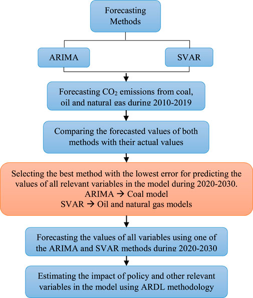
FIGURE 1. Conceptual framework of the study.

4 Model estimation

4.1 Determining the optimal lags length

After determining the variable for each model, in the next step, we examine the stationary state of the variables. In this study, the Augmented Dickey-Fuller and the Phillips-Perron tests were used to examine the stationary of variables. The results of these tests are reported in Table 1.

TABLE 1

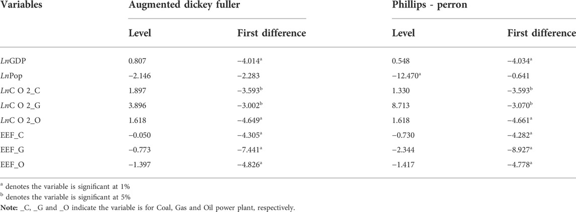
TABLE 1. Result for the unit root test.

Table 2 shows that among the study variables, only the population (POP) is stationary at its level and the other variables are not stationary at their level, but they have been stationary in their first differences. To determine the optimal lag length, we can use the criteria of the likelihood ratio (LR), Akaike (AIC), Schwartz (SC) and Hannan-Quinn (HQ) tests. The results of these tests are reported in Table 2.

TABLE 2

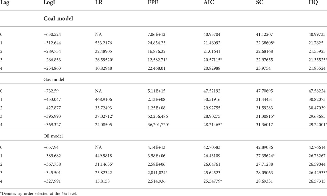
TABLE 2. Results for the optimal lag length for each model.

According to Table 2, the Schwartz criterion shows one lag for the coal model, three lags for the gas model and one lag for the oil model.

4.2 Co-integration test

The purpose of estimating the VAR model is to determine the number of long-run relationships between the model variables. Since the model consists of three variables, it is possible to have at least two long-run relationships between them. To test this problem using the Johansen’s method, the maximum eigenvalue and the trace statistics were used. The results of these statistics for each one of the models are presented in Table 3. As can be seen in this table, both the trace statistic and the maximum eigenvalue confirm the existence of at least one long-run relationship between the variables of each one of the models at the 95% confidence level. Therefore, we have estimated a long-run relationship under the Johansen model.

TABLE 3

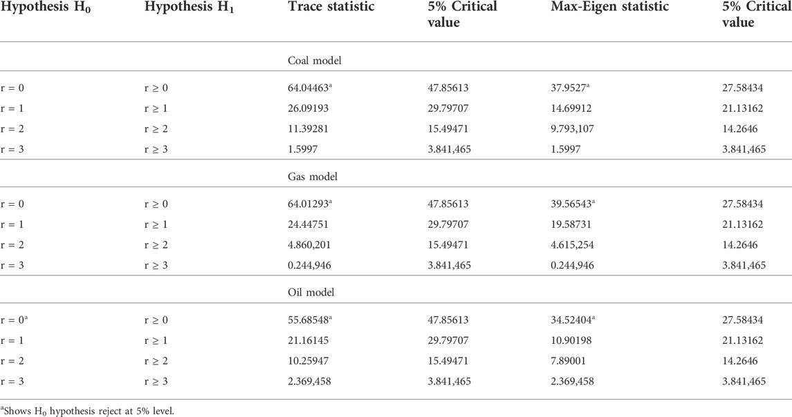
TABLE 3. Results for selection the order of co-integration.

4.3 Johansen model estimation

The Johansen model shows the long-run relationships and is helpful for policymaking. In addition, according to Table 4, the long-run relationships for each model is one, which is stated below. In addition, all variables are considered independent in this regard.

$\mathit{ln}\mathit{C}{\mathit{O}}_{\mathbf{2}}\mathbf{\_}{\mathit{C}}_{\mathit{t}}\mathbf{=}{\mathit{\alpha }}_{\mathbf{1}}\mathit{ln}\mathit{G}\mathit{D}{\mathit{P}}_{\mathit{t}}\mathbf{+}{\mathit{\alpha }}_{\mathbf{2}}\mathit{ln}\mathit{P}\mathit{O}{\mathit{P}}_{\mathit{t}}\mathbf{+}{\mathit{\alpha }}_3\mathit{E}\mathit{E}\mathit{F}\mathbf{\_}{\mathit{C}}_{\mathit{t}}(11)$

$\mathit{ln}\mathit{C}{\mathit{O}}_{\mathbf{2}}\mathbf{\_}{\mathit{G}}_{\mathit{t}}\mathbf{=}{\mathit{\beta }}_{\mathbf{1}}\mathit{ln}\mathit{G}\mathit{D}{\mathit{P}}_{\mathit{t}}\mathbf{+}{\mathit{\beta }}_{\mathbf{2}}\mathit{ln}\mathit{P}\mathit{O}{\mathit{P}}_{\mathit{t}}\mathbf{+}{\mathit{\beta }}_3\mathit{E}\mathit{E}\mathit{F}\mathbf{\_}{\mathit{G}}_{\mathit{t}}(12)$

$\mathit{ln}\mathit{C}{\mathit{O}}_{\mathbf{2}}\mathbf{\_}{\mathit{O}}_{\mathit{t}}\mathbf{=}{\mathit{\gamma }}_{\mathbf{1}}\mathit{ln}\mathit{G}\mathit{D}{\mathit{P}}_{\mathit{t}}\mathbf{+}{\mathit{\gamma }}_{\mathbf{2}}\mathit{ln}\mathit{P}\mathit{O}{\mathit{P}}_{\mathit{t}}\mathbf{+}{\mathit{\gamma }}_3\mathit{E}\mathit{E}\mathit{F}\mathbf{\_}{\mathit{O}}_{\mathit{t}}(13)$

TABLE 4

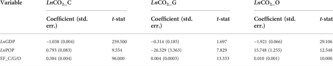
TABLE 4. Results for the Johansen model.

The results show that in the long run, real GDP has a negative and significant relationship with CO₂ emissions for each model. These results also show that, in the long run, there is a significant relationship between population and the CO₂ emissions. This model shows a significant relationship between the energy efficiency of each energy and CO₂ emissions from the combustion of each fuel. This means that their coefficients are reliable at the 1% level of significance, except for the real GDP in the natural gas model.

4.4 ARIMA model’s estimation

Another methodology used in this study is the autoregressive integrated moving average (ARIMA) model. The estimation of ARIMA models involves four main steps. The first step is the model’s identification. The identification step in estimating ARIMA models is made using the autocorrelation function (ACF) and the partial autocorrelation function (PACF). One of the prerequisites for the ARIMA model is the nonstationary condition of the variable under consideration. The third step in the ARIMA method is the model’s evaluation. Normally, at this stage, estimates with higher degrees are made and the best model is selected from them according to Akaike and Schwartz criteria as well as the white noise of the residual terms. The Akaike and Schwartz criteria were used to select the appropriate model, upon which the ARIMA (1,1,4) model, ARIMA (4,1,1) and ARIMA (6,1,10) were selected for coal, natural gas and oil models, respectively. However, since the main purpose of estimating these patterns is prediction, the amount of prediction error is more important in selecting the model. Detailed results of the ARIMA estimates are presented in Table 5.

TABLE 5

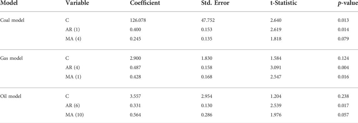
TABLE 5. Results for the ARIMA model.

In Table 5, for the coal model, the first-order, AR (1), and the fourth order of the autoregressive sentence, AR (4), are statistically significant. For the natural gas model, the fourth order, AR (4), and the first order, MA (1), are statistically significant and for the oil model, the sixth order, AR (6), and the 10th order, MA (10), are statistically significant.

4.5 Comparing the prediction power of VAR and ARIMA models

In the previous sections, CO₂ emissions from burning coal, natural gas and oil in power plants were estimated using the VAR and ARIMA methods. Based on these methods, the forecasted values of CO₂ emissions and their actual values for each model during 2010–2019 are presented in Tables 6 and 7. In this section, we compare the dual estimates of each model and check which one of them has greater predictive power. To do this, three criteria were used: the sum of squares error (MSE), the mean absolute value of error (MAE) and the mean absolute percentage error (MAPE).

TABLE 6

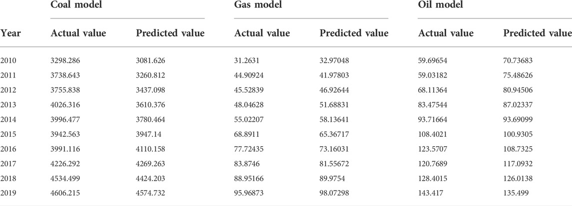
TABLE 6. Actual and residual values of the VAR model.

TABLE 7

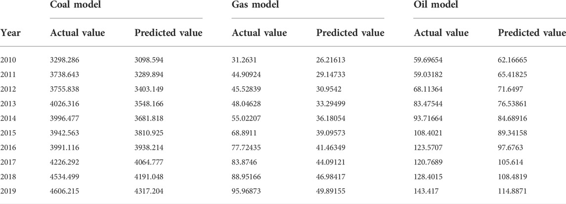
TABLE 7. Actual and residual values of the ARIMA model.

We now turn to the question of which of the two forecasting methods for each model has the least error? To answer this question, we compare the actual data and the predicted values of these two methods over the last 10 years (2010–2019), and determine the one with the least error. Meanwhile, the longer the forecast period, the greater the prediction error because the prediction of each period also contains the sum of the prediction error of the past. To determine the small amount of prediction errors, as mentioned above, the MSE, MAE and MAPE measures were used. The results of these measures are reported in Table 8.

TABLE 8

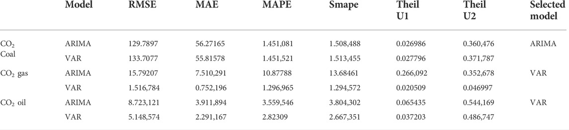
TABLE 8. Comparing the power of both ARIMA and VAR model in predicting CO₂ emissions.

The evaluation of the predictive power of the VAR model and its comparison with the ARIMA model indicates the difference in the accuracy of this model compared to another model. As shown in Table 8, the VAR model has the least error in predicting CO₂ emissions in the oil and natural gas models. However, in the prediction of CO₂ emissions from the coal power plant, the ARIMA model has the least prediction error.

4.6 CO₂ emissions forecast

For oil and natural gas models, the prediction criterion is the VAR model and for the coal model, the prediction criterion is the ARIMA model. Therefore, using these methods, we have predicted CO₂ emissions from combustion of coal, oil and natural gas over the 2020–2030 period. The results of these forecasts are presented in Figure 2, which shows that CO₂ emissions have increased over the relevant years.

FIGURE 2

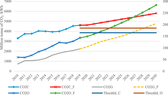
FIGURE 2. Predicted trends of CO₂ emissions created by different power plants during 2020–2030.

As Figure 2 shows, CO₂ emissions are increasing for all power plants, but from 2025 the rate of the increase in the coal-fired power plant will be slower. In 2029 and 2030, the gap between CO₂ emissions will be at a minimum, and this could be a promise to reduce CO₂ emissions from power generation in China’s coal-fired power plants, which make a very large share of coal-fired electricity generation.

5 Main results of the study

Before estimating the models, we need to find out the long-run relationship between the variables of each model using the bounds test. The value of the F-statistic of this test is compared to the criteria of the Narayan and Smyth (2005) study. If it is above the upper limit of the Narayan and Smyth (2005) criteria, it shows the long-run co-integration relationship between the variables. However, if it falls below the lower limit of the criterion, it does not show any long-run co-integration relationship. Finally, if it falls between the lower and upper limits, the value of the F-statistic will not be definitive. The results of the bounds test of all models in Table 9 show that there exists a long-run co-integration relationship between variables in each model.

TABLE 9

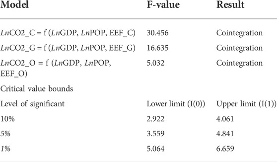
TABLE 9. Results for the bounds tests of all three models.

After finding a long-run co-integration relationship between the variables within each model, we estimate the short- and long-run impacts of each variable on CO₂ emissions. Table 10 shows the short and long-run results for the coal power plant. The results show that GDP has a positive and significant impact on CO₂ emissions from coal power plants in the short- and long-run. It shows that if real GDP increases by 1%, CO₂ emissions from coal power plants increase by 0.98 and 0.99% respectively in the short- and long-run. The population also has a positive impact on the coal power plant in both the short- and long-run, while its coefficient is not statistically significant. The coefficient of the energy efficiency in the coal power plants shows a negative and statistically significant impact on CO₂ emissions from coal power plants in the short and long run. This means that with an increase of 1% in energy efficiency, CO₂ emissions from coal power plants decline by 0.34 and 0.36% respectively in the short- and long-run. The coefficient of the dummy variable has a negative sign and is statistically significant only in the long run. It shows that the emissions trading scheme can reduce the CO₂ emissions from the coal power plant in the long run.

TABLE 10

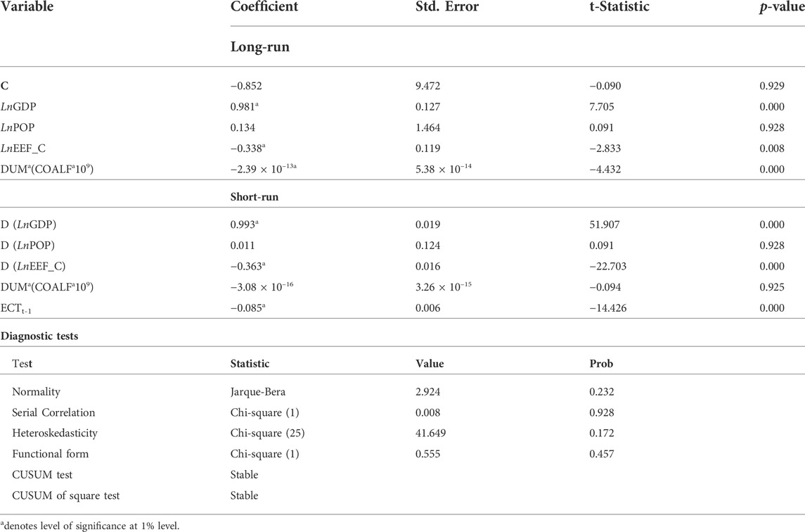
TABLE 10. ARDL results for the Coal power plant (dependent variable = CO2_C).

Table 11 reports the short- and long-run results for the natural gas power plants. The results show that GDP has a positive and statistically significant impact on the CO₂ emissions from the combustion of natural gas in power plants in the short- and long-run. It shows that if real GDP increases by 1%, CO₂ emissions from natural gas power plants increase by 1.53 and 0.76% in the short- and long-run, respectively. The coefficient of the population has a negative impact on natural gas power plants in the short- and long-run, but it is not statistically significant. The coefficient of the energy efficiency in the natural gas power plants shows a negative and statistically significant impact on the CO₂ emissions of natural gas power plants in the short- and long-run. This means that with an increase of 1% in energy efficiency, CO₂ emissions of natural gas power plants decline by 0.003% in the short- and long-run. The coefficient of the dummy variable has a negative sign and is statistically significant in the short and long run. It shows that the emissions trading scheme can reduce the CO₂ emissions from natural power plants in the short and long run.

TABLE 11

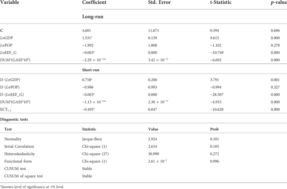
TABLE 11. ARDL results for the Gas power plant (dependent variable = CO2_G).

Table 12 provides the short- and long-run results for the oil power plants. The results show that GDP has a positive and statistically significant impact on the CO₂ emissions from the combustion of oil in power plants in the short- and long-run. It shows that if real GDP increases by 1%, CO₂ emissions from oil power plants will increase by 1.56 and 1.29% in the short- and long-run, respectively. The coefficient of the population has a negative and statistically significant impact on oil power plants in both the short- and long-run. It shows that if the population increases by 1%, CO₂ emissions from oil power plants declines by 9.80 and 4.27% in the short- and long-run, respectively. This may occur due to the increase in the use of more clean energies like natural gas in the combined oil and natural gas power plants. The coefficient of the energy efficiency in the oil power plants shows a negative and statistically significant impact on CO₂ emissions from oil power plants in the short- and long-run. This means that with an increase of 1% in energy efficiency, CO₂ emissions from oil power plants decline by 0.01% in the short- and long-run. The coefficient of the dummy variable has a negative sign and is statistically significant only in the long run. It shows that the emissions trading scheme can only reduce the CO₂ emissions from the oil power plants in the long-run.

TABLE 12

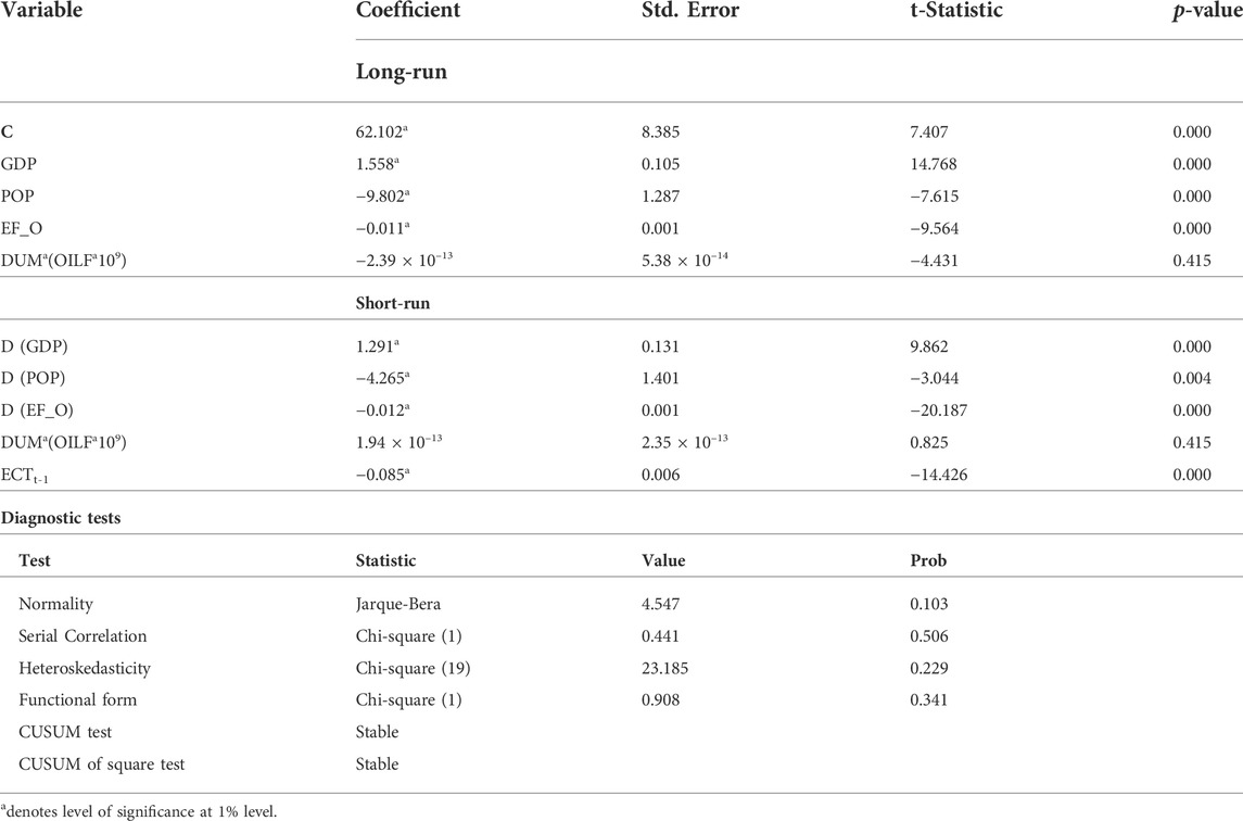
TABLE 12. ARDL results for the Oil power plant (dependent variable = CO2_O).

6 Discussion

The level of energy consumption cannot be significantly reduced through the increase in energy prices due to the low elasticity of demand for energy. Therefore, economic and population growth are the main contributors to high demand for energy and electricity (Solaymani et al., 2015). Therefore, other policies and motivation methods aimed at increasing energy efficiency and the use of renewable energy sources can help to use fossil fuel power plants in China and other countries.

One of the China’s most important sources of CO₂ emissions is its GDP. The results show that GDP positively and significantly increases CO₂ emissions in the short- and long-run. This means that economic growth and its components, such as trade, due to more use of fossil fuels increase CO₂ and other pollutants in the environment. This is consistent with the study conducted by Solaymani (2020), Mohsin et al. (2022) and Solaymani and Shokrinia (2016). The population has a negative impact on CO₂ emissions from natural gas power plants. This is because more use of natural gas instead of other fossil fuels in the economy, particularly by households, reduces the level of CO₂ emissions. This is not consistent with the overall finding of studies that have shown that the population increases CO₂ emissions in the overall economy, such as Li and Solaymani (2021). Improving energy efficiency in all power plants reduces CO₂ emissions from the combustion of coal, oil and natural gas in related power plants. Ponce and Khan, (2021) and Mahi et al. (2021) showed that energy efficiency reduces CO₂ emissions significantly. Peng et al. (2021) also showed that energy efficiency improvement reduces CO₂ emissions. Evidence also showed that the emissions trading scheme has a significant and negative impact on CO₂ emissions from the combustion of coal, oil and natural gas in relevant power plants. This finding supports the results of the study conducted by Huang et al. (2021) argued that this policy can reduce CO₂ emissions while it may have a negative impact on the economic performance of China. Mo (2021) also showed that the emission trading scheme (ETS) has been promoted as a cost-effective market-based reduction tool.

7 Conclusion and policy implications

This purpose of this study was to predict the impact of the emissions trading scheme on CO₂ emissions from the combustion of coal, oil and natural gas in electricity generation in power plants using annual data from 1985 to 2019. For this purpose, this study first chooses the best technique between ARIMA and structural Vector Autoregression (SVAR) techniques to predict CO₂ emissions, electricity generation from coal, oil and natural gas, efficiencies of coal, oil and natural gas and other relevant variables over the 2020–2030 period. Then by employing the ARDL methodology and using the predicted values of the study variables, we estimated the short- and long-run impacts of the policy on CO₂ emissions from the combustion of coal, oil and natural gas in electricity generation over the projected period (2020–2030). To estimate the impact of the policy on CO₂ emissions, we used a dummy variable for the forecast period, which is multiplied by the average threshold value of the policy.

The results of this study showed that real GDP has a significant and positive impact on CO₂ emissions from the combustion of all fuels (coal, oil and natural gas) in the short- and long-run. Energy efficiency also has a negative and significant impact on CO₂ emissions from all power plants in the short- and long-run. The results also suggest that the ETS policy is effective in reducing the CO₂ emissions from the combustion of all fuels in electricity production in the long-run. These results suggest that improving the efficiency of all fuels can significantly reduce the level of CO₂ emissions from coal, oil and natural gas in electricity generation in the short- and long-run. This is because of the increase in the level of CO₂ emissions from these power plants in the long-run, which exceed the threshold value. But it has a negative and statistically significant impact only on the CO₂ emissions from the natural gas power plants in the short-run. The results of the study enable Chinese energy policymakers to update the ETS policy in its next phases.

It is recommended that the China’s ETS policy needs to be expand to the majority of industries, particularly those with high carbon emissions. Since China has other environmental policies and regulations, a master plan for all need to be prepared and combined. The government’s programs for environmental protection must stimulate clean and high-tech industries. The government needs to pay more attention to the differences between industries and regions and prepare effective and appropriate policies and programs for each. The main limitation of the emission trading scheme investigation is the availability of microdata on the amount of emission of major carbon emitting industries and their economic performance. Improvements in the availability of microdata are also recommended.

For future studies, we recommend the use of more appropriate and relevant variables in the modeling to predict the impact of the ETS policy on CO₂ emissions. the use of other econometric methods, such as panel data, is also recommended to predict the impact of the ETS policy on different region or industry.

Data availability statement

Publicly available datasets were analyzed in this study. This data can be found here: The world bank indicators and US Energy Information Administration (EIA).

Author contributions

The author confirms being the sole contributor of this work and has approved it for publication.

Conflict of interest

The author declares that the research was conducted in the absence of any commercial or financial relationships that could be construed as a potential conflict of interest.

Publisher’s note

All claims expressed in this article are solely those of the authors and do not necessarily represent those of their affiliated organizations, or those of the publisher, the editors and the reviewers. Any product that may be evaluated in this article, or claim that may be made by its manufacturer, is not guaranteed or endorsed by the publisher.

Abbreviations

CO2, carbon dioxide emissions; SO2, sulfur dioxide; ETS, Emissions Trading Scheme; SVAR, structural Vector Auto-regression; ARIMA, autoregressive integrated moving average; ARDL, Autoregressive distributed lag; GDP, gross domestic product; EEF, energy efficiency; POP, population.

References

Akram, R., Chen, F., Khalid, F., Ye, Z., and Majeed, M. T. (2020). Heterogeneous effects of energy efficiency and renewable energy on carbon emissions: Evidence from developing countries. J. Clean. Prod. 247, 119122. doi:10.1016/j.jclepro.2019.119122

CrossRef Full Text | Google Scholar

Chang, K., Ge, F., Zhang, C., and Wang, W. (2018). The dynamic linkage effect between energy and emissions allowances price for regional emissions trading scheme pilots in China. Renew. Sustain. Energy Rev. 98, 415–425. doi:10.1016/j.rser.2018.09.023

CrossRef Full Text | Google Scholar

Chen, Z., Yuan, X-C., Zhang, X., and Cao, Y. (2020). How will the Chinese national carbon emissions trading scheme work? The assessment of regional potential gains. Energy Policy 137, 111095. doi:10.1016/j.enpol.2019.111095

CrossRef Full Text | Google Scholar

Cui, L-B., Fan, Y., Zhu, L., and Bi, Q-H. (2014). How will the emissions trading scheme save cost for achieving China’s 2020 carbon intensity reduction target? Appl. Energy 136, 1043–1052. doi:10.1016/j.apenergy.2014.05.021

CrossRef Full Text | Google Scholar

Dai, H., Xie, Y., Liu, J., and Masui, T. (2018). Aligning renewable energy targets with carbon emissions trading to achieve China's INDCs: A general equilibrium assessment. Renew. Sustain. Energy Rev. 82 (3), 4121–4131. doi:10.1016/j.rser.2017.10.061

CrossRef Full Text | Google Scholar

de Souza Mendonça, A. K., de Andrade Conradi Barni, G., Moro, M. F., Bornia, A. C., Kupek, E., and Fernandes, L. (2020). Hierarchical modeling of the 50 largest economies to verify the impact of GDP, population and renewable energy generation in CO₂ emissions. Sustain. Prod. Consum. 22, 58–67. doi:10.1016/j.spc.2020.02.001

CrossRef Full Text | Google Scholar

Feng, T-T., Yang, Y-S., and Yang, Y-H. (2018). What will happen to the power supply structure and CO₂ emissions reduction when TGC meets CET in the electricity market in China? Renew. Sustain. Energy Rev. 92, 121–132. doi:10.1016/j.rser.2018.04.079

CrossRef Full Text | Google Scholar

Grubb, M., and Neuhoff, K. (2010). Allocation and competitiveness in the EU emissions trading scheme: Policy overview. Clim. Policy 6 (1), 7–30. doi:10.1080/14693062.2006.9685586

CrossRef Full Text | Google Scholar

Huang, J., Shen, J., Miao, L., and Zhang, W. (2021). The effects of emission trading scheme on industrial output and air pollution emissions under city heterogeneity in China. J. Clean. Prod. 315, 128260. doi:10.1016/j.jclepro.2021.128260

CrossRef Full Text | Google Scholar

International Energy Agency (IEA) (2021). The role of China’s ETS in power sector decarbonisation. Paris, France: International Energy Agency.

Google Scholar

Jotzo, F., Karplus, V., Grubb, M., Loschel, A., Neuhoff, K., Wu, L., et al. (2018). China’s emissions trading takes steps towards big ambitions. Nat. Clim. Chang. 8, 265–267. doi:10.1038/s41558-018-0130-0

CrossRef Full Text | Google Scholar

Jotzo, F., and Löschel, A. (2014). Emissions trading in China: Emerging experiences and international lessons. Energy Policy 75, 3–8. doi:10.1016/j.enpol.2014.09.019

CrossRef Full Text | Google Scholar

Laing, T., Sato, M., Grubb, M., and Comberti, C. (2014). The effects and side-effects of the EU emissions trading scheme. WIREs Clim. Change 5, 509–519. doi:10.1002/wcc.283

CrossRef Full Text | Google Scholar

Li, W., Zhang, Y-W., and Lu, C. (2018). The impact on electric power industry under the implementation of national carbon trading market in China: A dynamic CGE analysis. J. Clean. Prod. 200, 511–523. doi:10.1016/j.jclepro.2018.07.325

CrossRef Full Text | Google Scholar

Li, Y., and Solaymani, S. (2021). Energy consumption, technology innovation and economic growth nexuses in Malaysian. Energy 232, 121040. doi:10.1016/j.energy.2021.121040

CrossRef Full Text | Google Scholar

Lin, B., and Jia, Z. (2019). What will China's carbon emission trading market affect with only electricity sector involvement? A CGE based study. Energy Econ. 78, 301–311. doi:10.1016/j.eneco.2018.11.030

CrossRef Full Text | Google Scholar

Liu, C., Ma, C., and Xie, R. (2020). Structural, innovation and efficiency effects of environmental regulation: Evidence from China’s carbon emissions trading pilot. Environ. Resour. Econ. (Dordr). 75, 741–768. doi:10.1007/s10640-020-00406-3

CrossRef Full Text | Google Scholar

Liu, M., Zhou, C., Lu, F., and Hu, X. (2021). Impact of the implementation of carbon emission trading on corporate financial performance: Evidence from listed companies in China. PLoS ONE 16 (7), e0253460. doi:10.1371/journal.pone.0253460

PubMed Abstract | CrossRef Full Text | Google Scholar

Liu, X., Wang, B., Du, M., and Zhang, N. (2018). Potential economic gains and emissions reduction on carbon emissions trading for China's large-scale thermal power plants. J. Clean. Prod. 204, 247–257. doi:10.1016/j.jclepro.2018.08.131

CrossRef Full Text | Google Scholar

Liu, Z., and Sun, H. (2021). Assessing the impact of emissions trading scheme on low-carbon technological innovation: Evidence from China. Environ. Impact Assess. Rev. 89, 106589. doi:10.1016/j.eiar.2021.106589

CrossRef Full Text | Google Scholar

Lu, M., Wang, Y., and Wang, X. (2021). Impact of China carbon emissions trading mechanism on industrial competitiveness: Evidence from Beijing. IOP Conf. Ser. Earth Environ. Sci. 657, 012105. doi:10.1088/1755-1315/657/1/012105

CrossRef Full Text | Google Scholar

Ma, B., Liu, p., and Niu, D. (2018). Assessment of power industry development in China: Possibilities and challenges. J. Renew. Sustain. Energy 10, 045903. doi:10.1063/1.5033478

CrossRef Full Text | Google Scholar

Ma, Q., Yan, G., Ren, X., and Ren, X. (2022). Can China’s carbon emissions trading scheme achieve a double dividend? Environ. Sci. Pollut. Res. 29, 50238–50255. doi:10.1007/s11356-022-19453-y

CrossRef Full Text | Google Scholar

Mahi, M., Ismail, I., Phoong, S. W., and Isa, C. R. (2021). Mapping trends and knowledge structure of energy efficiency research: What we know and where we are going. Environ. Sci. Pollut. Res. 28, 35327–35345. doi:10.1007/s11356-021-14367-7

PubMed Abstract | CrossRef Full Text | Google Scholar

Mikayilov, J. I., Hasanov, F. J., and Galeotti, M. (2018). Decoupling of CO₂ emissions and GDP: A time-varying cointegration approach. Ecol. Indic. 95 (1), 615–628. doi:10.1016/j.ecolind.2018.07.051

CrossRef Full Text | Google Scholar

Mo, J. Y. (2021). Technological innovation and its impact on carbon emissions: Evidence from korea manufacturing firms participating emission trading scheme. Technol. Analysis Strategic Manag. 34 (1), 47–57. doi:10.1080/09537325.2021.1884675

CrossRef Full Text | Google Scholar

Mohsin, M., Naseem, S., Sarfraz, M., and Azam, T. (2022). Assessing the effects of fuel energy consumption, foreign direct investment and GDP on CO₂ emission: New data science evidence from Europe & Central Asia. Fuel 314, 123098. doi:10.1016/j.fuel.2021.123098

CrossRef Full Text | Google Scholar

Narayan, P. K., and Smyth, R. (2005). Electricity consumption, employment and real income in Australia evidence from multivariate Granger causality tests. Energy Policy 33, 1109–1116. doi:10.1016/j.enpol.2003.11.010

CrossRef Full Text | Google Scholar

Oliveira, T. D., Gurgel, A. C., and Tonry, S. (2021). Potential trading partners of a Brazilian emissions trading scheme: The effects of linking with a developed region (Europe) and two developing regions (Latin America and China). Technol. Forecast. Soc. Change 171, 120947. doi:10.1016/j.techfore.2021.120947

CrossRef Full Text | Google Scholar

Peng, H., Qi, S., and Cui, J. (2021). The environmental and economic effects of the carbon emissions trading scheme in China: The role of alternative allowance allocation. Sustain. Prod. Consum. 28, 105–115. doi:10.1016/j.spc.2021.03.031

CrossRef Full Text | Google Scholar

Pesaran, M. H., Shin, Y., and Smith, R. J. (2001). Bounds testing approaches to the analysis of level relationships. J. Appl. Econ. Chichester. Engl. 16 (3), 289–326. doi:10.1002/jae.616

CrossRef Full Text | Google Scholar

Ponce, P., and Khan, S. A. R. (2021). A causal link between renewable energy, energy efficiency, property rights, and CO2 emissions in developed countries: A road map for environmental sustainability. Environ. Sci. Pollut. Res. 28, 37804–37817. doi:10.1007/s11356-021-12465-0

CrossRef Full Text | Google Scholar

Rahman, M. M., Saidi, K., and Mbarek, M. B. (2020). Economic growth in south asia: The role of CO₂ emissions, population density and trade openness. Heliyon 6 (5), e03903. doi:10.1016/j.heliyon.2020.e03903

PubMed Abstract | CrossRef Full Text | Google Scholar

Razzaq, A., Sharif, A., Najmi, A., Tseng, M-L., and Lim, M. K. (2021). Dynamic and causality interrelationships from municipal solid waste recycling to economic growth, carbon emissions and energy efficiency using a novel bootstrapping autoregressive distributed lag. Resour. Conservation Recycl. 166, 105372. doi:10.1016/j.resconrec.2020.105372

CrossRef Full Text | Google Scholar

Solaymani, S. (2020). A CO₂ emissions assessment of the green economy in Iran. Greenh. Gas. Sci. Technol. 10 (2), 390–407. doi:10.1002/ghg.1969

CrossRef Full Text | Google Scholar

Solaymani, S. (2022). CO₂ emissions and the transport sector in Malaysia. Front. Environ. Sci. 9, 774164. doi:10.3389/fenvs.2021.774164

CrossRef Full Text | Google Scholar

Solaymani, S., Najafi, S. M. B., Kari, F., and Satar, N. B. M. (2015). Aggregate and regional demand for electricity in Malaysia. J. energy South. Afr. 26 (1), 46–54. Available at: http://www.scielo.org.za/scielo.php?script=sci_arttext&pid=S1021-447X2015000100006&lng=en&tlng=en.

CrossRef Full Text | Google Scholar

Solaymani, S., and Shokrinia, M. (2016). Economic and environmental effects of trade liberalization in Malaysia. J. Soc. Econ. Dev. 18, 101–120. doi:10.1007/s40847-016-0023-x

CrossRef Full Text | Google Scholar

Tan, Q., Mei, S., Ye, Q., Ding, Y., and Zhang, Y. (2019). Optimization model of a combined wind-PV-thermal dispatching system under carbon emissions trading in China. J. Clean. Prod. 225, 391–404. doi:10.1016/j.jclepro.2019.03.349

CrossRef Full Text | Google Scholar

Tang, K., Zhou, Y., Liang, X., and Zhou, D. (2021). The effectiveness and heterogeneity of carbon emissions trading scheme in China. Environ. Sci. Pollut. Res. 28, 17306–17318. doi:10.1007/s11356-020-12182-0

CrossRef Full Text | Google Scholar

Verde, S., Galdi, G., Alloisio, I., and Borghesi, S. (2021). The EU ETS and its companion policies: Any insight for China's ETS? Environ. Dev. Econ. 26 (3), 302–320. doi:10.1017/s1355770x20000595

CrossRef Full Text | Google Scholar

Wen, H-X., Chen, Z-R., and Nie, P-Y. (2021). Environmental and economic performance of China’s ETS pilots: New evidence from an expanded synthetic control method. Energy Rep. 7, 2999–3010. doi:10.1016/j.egyr.2021.05.024

CrossRef Full Text | Google Scholar

Xiao, J., Li, G., Zhu, B., Xie, L., Hu, Y., and Huang, J. (2021). Evaluating the impact of carbon emissions trading scheme on Chinese firms’ total factor productivity. J. Clean. Prod. 306, 127104. doi:10.1016/j.jclepro.2021.127104

CrossRef Full Text | Google Scholar

Zeng, B., Xie, J., Zhang, X., Yu, Y., and Zhu, L. (2020). The impacts of emission trading scheme on China’s thermal power industry: A pre-evaluation from the micro level. Energy & Environ. 31 (6), 1007–1030. doi:10.1177/0958305x19882388

CrossRef Full Text | Google Scholar

Zhang, G., Zhang, N., and Liao, W. (2018). How do population and land urbanization affect CO₂ emissions under gravity center change? A spatial econometric analysis. J. Clean. Prod. 202, 510–523. doi:10.1016/j.jclepro.2018.08.146

CrossRef Full Text | Google Scholar

Zhang, K., Xu, D., Li, S., Zhou, N., and Xiong, J. (2018). Has China’s pilot emissions trading scheme influenced the carbon intensity of output? Int. J. Environ. Res. Public Health 16 (10), 1854. doi:10.3390/ijerph16101854

CrossRef Full Text | Google Scholar

Zhang L, L., Li, Y., and Jia, Z. (2018). Impact of carbon allowance allocation on power industry in China’s carbon trading market: Computable general equilibrium based analysis. Appl. Energy 229, 814–827. doi:10.1016/j.apenergy.2018.08.055

CrossRef Full Text | Google Scholar

Zhang, W., Li, G., and Guo, F. (2022). Does carbon emissions trading promote green technology innovation in China? Appl. Energy 315, 119012. doi:10.1016/j.apenergy.2022.119012

CrossRef Full Text | Google Scholar

Zheng, Y., Sun, X., Zhang, C., Wang, D., and Mao, J. (2021). Can emission trading scheme improve carbon emission performance? Evidence from China. Front. Energy Res. 9, 759572. doi:10.3389/fenrg.2021.759572

CrossRef Full Text | Google Scholar