 Huan Long
 Runhao Geng1
94% of researchers rate our articles as excellent or good
Learn more about the work of our research integrity team to safeguard the quality of each article we publish.
Find out more
ORIGINAL RESEARCH article
Front. Energy Res., 15 July 2022
Sec. Smart Grids
Volume 10 - 2022 | https://doi.org/10.3389/fenrg.2022.954274
This article is part of the Research TopicEngineering Applications of Neurocomputing Volume IIView all 6 articles
This study proposes a combination interval prediction based hybrid ensemble (CIPE) model for short-term wind speed prediction. The combination interval prediction (CIP) model employs the extreme learning machine (ELM) as the predictor with a biased convex cost function. To relieve the heavy burden of the hyper-parameter selection of the biased convex cost function, a hybrid ensemble technique is developed by combining the bagging and stacking ensemble methods. Multiple CIP models with random hyper-parameters are first trained based on the sub-datasets generated by the bootstrap resampling. The linear regression (LR) is utilized as the meta model to aggregate the CIP models. By introducing the binary variables, the LR meta model can be formulated as a mixed integer programming (MIP) problem. With the benefit of the biased convex cost function and ensemble technique, the high computational efficiency and stable performance of the proposed prediction model is guaranteed simultaneously. Multi-step ahead 10-min wind speed interval prediction is conducted based on actual wind farm data. Comprehensive experiments are carried out to verify the superiority of the proposed interval prediction model.
Wind energy, as a clean and renewable energy resource, has been widely utilized and highly valued in recent years. However, due to its high intermittency and variability, the application of wind power brings considerable uncertainties to modern power systems (Li, 2022a). Forecasting wind power output intrinsically relies on estimates of wind speed. Effective and reliable prediction of the short-term wind speed can assist the timely adjustment of the scheduling plan, reduce cost impact on power system operators, and aid the integration of wind energy in the electricity system (Zhang et al., 2020). Traditional point prediction only provides the deterministic predicted value (Li, 2022b). Compared with point prediction, interval prediction is capable of quantifying the uncertainty by constructing fluctuation intervals for wind speed (Li et al., 2020a). Therefore, interval prediction with a certain confidence is meaningful for offering a comprehensive reference to the relevant decision-making issues of power systems (Li et al., 2021a).
The interval prediction pays more attention to the boundary information compared to the point prediction. Among the various interval prediction methods, the lower and upper bound estimation (LUBE) method as a nonparametric approach becomes one of the mainstream methods. In (Khosravi et al., 2011), the LUBE employing a double-output neural network with the performance index coverage width-based criterion (CWC) was first proposed to directly construct the prediction interval (PI). Cost function is one of the improvement directions in the subsequent works. In (Wan et al., 2014), the winkler score was revised and combined with coverage deviation to substitute CWC. In the study by (Shrivastava et al., 2016), the interval width and coverage rate of PIs were separately optimized to train the LUBE by utilizing the multi-objective differential evolution algorithm. In the study by (Kavousi-Fard et al., 2016), a fuzzy-based cost function was introduced into the LUBE framework, and the PI combination approach was applied to further improve reliability and flexibility. In the study by (Hu et al., 2017), three indices, deviation of the coverage rate, deviation of PI from uncovered targets, and interval width were viewed as optimization objectives, further improving the prediction performance of multi-objective optimization. In the study by (Liu et al., 2020), a continuous and differential cost function was proposed, making a gradient descent training mechanism feasible in the LUBE framework. With the development of deep learning, some works aimed to improve the performance of LUBE from the perspective of a prediction engine. Various deep neural networks were also introduced into LUBE to further enhance the performance, such as recurrent neural networks (Shi et al., 2018) and long short-term memory networks (Banik et al., 2020).
In the above references (Khosravi et al., 2011), (Hu et al., 2017), (Shi et al., 2018), (Banik et al., 2020), the LUBE model was usually trained by the heuristic algorithm due to the non-differentiability of the cost function, which introduced the heavy computational cost and unstable performance. To address this problem, a biased convex cost function was proposed in the study by (Long et al., 2021), which comprises error term and penalty term to comprehensively evaluate the quality of PI. Due to the differentiability and convexity, the convex optimization could be utilized to train the LUBE model instead of heuristic algorithm. However, the model performance depends on enumeration and combination of the hyper-parameters, to which the performance of the proposed biased convex cost function is related. Thus, complex hyper-parameter tuning seriously limits model training efficiency.
To relieve the heavy burden of hyper-parameter selection, ensemble techniques are applicable in this study. The ensemble mechanism combines several weak learners to generate a superior strong learner and does not have high requirements of base models (Xiyun et al., 20172017). The bagging ensemble is a simple and widely used ensemble method, which generates sub-datasets by bootstrap resampling to build base models and aggregate them by averaging or majority voting (Breiman, 1996). In the study by (Liu and Xu, 2020), the bootstrap resampling was also utilized to obtain empirical distributions of point prediction errors to construct PI. However, the average combination strategy of bagging is too simple to guarantee the prediction performance (Liu and Xu, 2020). High and stable prediction accuracy of the bagging ensemble model requires a large number of base models, which leads to great training time (Li et al., 2021b).
The stacking ensemble was first proposed by Wolpert to use a meta learner for aggregating heterogeneous base models, which transforms model aggregation into a new model training problem (Wolpert, 1992). Such transformation allows diverse forms of combination to improve the aggregation effect and relieves the requirement of the number of base models. In the study by (Massaoudi et al., 2021), a multi-layer perceptron was utilized as the meta learner to combine different base models for load prediction. In the study by (Moon et al., 2020), multiple deep neural network models were aggregated by the principle component regression based on the stacking ensemble structure. Thus, the meta learner mechanism of stacking ensemble is introduced into bagging to replace the average combination strategy to enhance the ensemble quality in this study.
To consider the computational efficiency of short-term prediction, the linear regression model is chosen as the meta model to combine PIs constructed by base models. In the study by (Zhao et al., 2020), the ELM, which was regarded as a nonparametric regression function, was formulated as a MIP problem by introducing the binary variable to mark whether the actual target covered by the PI. The quantile regression (Koenker and Bassett, 1978) was further used to cut down the number of the binary variables to improve the computational efficiency. Thus, the LR meta model in this study can also be formulated as a MIP problem through introducing the binary variable, by which the combination quality of PIs and the training efficiency of the meta model can be ensured simultaneously, and such formulation can be solved using the convex optimization technique.
This study proposes a CIP-based hybrid ensemble model, which combines bagging and stacking ensemble approaches. The CIP model with a biased convex cost function is constructed based on the LUBE interval prediction structure. To relieve the heavy burden of hyper-parameter selection, the ensemble technology is employed to cut down the number of hyper-parameters to three, which are the number of base models, the number of hidden neurons, and the value of the regularization coefficient. Multiple CIPs with random hyper-parameters of the biased convex cost function are selected as base models. Considering model performance and training efficiency, the LR model is chosen as the meta model to aggregate CIP base models, which can be formulated as a MIP problem by introducing binary variables. Multi-step ahead 10-min wind speed predictions with multiple coverage probability are investigated in this study, and comprehensive experiments are implemented based on realistic wind farm data to validate the performance of the proposed model.
In short, the main contributions of this study can be summarized as follows:
1) A hybrid ensemble model is proposed for wind speed interval prediction. The burden of tuning hyper-parameters of the biased cost function is relieved and the total number of hyper-parameters cuts down to three.
2) Stacking ensemble is introduced into bagging ensemble to reduce model complexity. The linear regression model is utilized as the combiner, which can be formulated as a MIP problem, to improve the model training time.
A prediction interval is composed of the upper and lower bounds that bracket a future unknown value with a prescribed empirical confidence level. In order to comprehensively evaluate the general performance of the PIs, coverage rate and interval width are served as the two criteria for the assessment. Given time-series sample set D =
The prediction interval coverage probability, PICP, measures the reliability of the PI, which is formulated by the proportion of the targets falling within the PIs in (1).
where
The prediction interval normalized average width, PINAW, represents the concentration degree of PI, expressed as (2).
where R denotes the range of the target value.
Generally, PI with high PICP and small PINAW is preferable. However, excessive pursuit of narrow width is prone to yielding unreliable PI with substandard coverage probability. Therefore, the performance of the PI is generally evaluated via comparing the PINAW under certain PICP.
The improved CWC index (Wang et al., 2020), shown in (3) and (4), provides a comprehensive evaluation of PI.
where PINRW denotes the prediction interval normalized root mean square width, which is expressed as (5), η1 is utilized to linearly increase the influence of PINRW, η2 is the penalty factor for PICP, and PINC represents the expected nominal coverage probability for the evaluation on the test dataset.
The proposed CIPE model is on the basis of the hybrid ensemble framework which combines bagging and stacking ensemble, displayed in Figure 1. In base model training, the bootstrap resampling is first utilized to generate different sub-datasets, D1, … , Dk, … , DK. The kth CIP base model is pre-trained using the convex optimization technique based on the Dk.
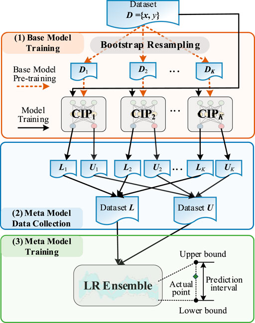
FIGURE 1. Framework of the CIPE model.
In meta model data collection, the whole dataset D is utilized by each pre-trained CIP base model to separately construct PI, which corresponds to the same time point. The predicted upper and lower bounds of each pre-trained CIP model are collected to generate the dataset U and L, which are the training data for meta models.
In meta model training, the LR model is employed to aggregate base models, which can be formulated as a MIP problem by introducing the binary variable to describe whether the target is covered by PI. The quantile regression is utilized to cut down the number of binary variables. To achieve the expected PICP and narrow PINAW, the sum of PI width with weight penalty is regarded as the objective and the expected PICP is considered as the constraint.
With the help of the ensemble mechanism, the values of hyper-parameters in each CIP base model are randomly generated. The heavy burden of the artificial selection of hyper-parameters in the CIP model is relieved. Besides, the combination of the bagging and stacking ensemble further enhances the generalization and robustness of the randomly generated base model. Thus, the computational efficiency and prediction performance can be achieved at the same time.
The CIP model is based on a double-output ELM prediction model (Long et al., 2021), shown as Figure 2. A biased convex cost function is proposed to obtain the output weight matrix for the upper and lower bounds, respectively. Different trained upper and lower bounds under different hyper-parameters of the proposed cost functions are combined. The optimal combination of the predicted upper and lower bounds with optimal hyper-parameters is optimized by minimizing the PINAW under the constraint of satisfying the expected PICP.
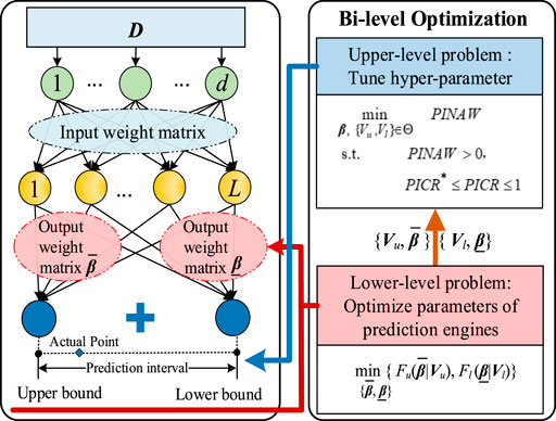
FIGURE 2. Structure of the CIP model.
Given the training dataset
where f(x) is the activation function while h(x) is the output vector of the hidden layer, and w and b are the input weight matrix and the bias vector of the hidden layer, respectively.
The lower and upper bounds of the PI can be defined as (7).
where
Since the actual value of li and ui are unknown, the
where W, r and c are the hyper-parameters of the biased cost function.
Each hyper-parameter of biased cost function E(∙) has a clear meaning which is directly related to the performance of PI. W is the coefficient of penalty term S(∙), which controls its proportion in E(∙). The hyper-parameter c is to alleviate the punishment on the predicted targets which exceed the predicted bound. Because 100% coverage probability is usually not the objective, it is not necessary to impose penalties on any violators. r amplifies the deviation θ, providing more degrees of freedom to E(∙).
Figure 3 graphically illustrates the effect of the hyper-parameters of E(∙). If θ > 0, the target exceeds the predicted bound. In Figure 3A, at θ = 0.5, the value of E(∙) increases to about 6 times the original value when W increases from 1 to 10. Thus, the increase in W leads to more penalties on the uncovered target such that the predicted bound can be quickly adjusted to cover it and PICP is improved. Similarly, apt changes of c and r are able to control the proportion of punishment to adjust the PICP.
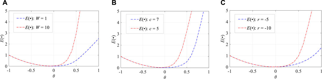
FIGURE 3. Illustration of the hyper-parameters of E(∙): (A) change on the value of W, (B) change on the value of c, and (C) change on the value of r.
Furthermore, the part where the red and blue lines overlap illustrates that the target is inside the predicted bound. The penalty term S(θ) almost disappears and error term θ2 is the main part of the function E(∙). In this condition, more attention is paid to reducing the distance between the target and predicted bound to decrease the interval width.
To improve the generalization performance of ELM, a regularization term is added. The specific formulation of the biased cost function of upper and lower bound output are presented as (10) and (11).
where Cu and Cl are the regularization coefficients, Vu = {Wu, ru, cu, Cu} is the hyper-parameter set for the upper bound, and Vl = {Wl, rl, cl, Cl} is the hyper-parameter set for the lower bound. To achieve narrow PINAW and satisfy the expected PICP, the selection of Vu and Vl should be optimized and the CIP model can be formulated as (12).
where PICP* denotes the pre-assigned nominal coverage probability for model training, and Θ represents the searching space of Vu and Vl. Since eight hyper-parameters need to be fine-tuned, grid search strategy is utilized. Multiple prediction boundaries corresponding to different hyper-parameters are generated, and the optimal PI is constructed via enumeration and combination. The hyper-parameter space is too large to search, and the optimal value is difficult to determine. Thus, the ensemble mechanism is introduced to reduce the heavy work of hyper-parameter selection by randomly generating the hyper-parameter values.
Bagging and stacking are two conventional ensemble methods. Bagging ensemble aggregates the multiple base models by averaging or majority voting. The base models are trained based on different sub-datasets generated by the bootstrap resampling. Stacking ensemble combines several heterogeneous base models using a meta model. Its general idea is to use the base models’ outputs along with real target values to train the meta model. Unlike bagging, stacking employs a certain learning algorithm as the combination strategy to train the combiner instead of simple averaging or voting methods. Thus, the stacking ensemble does not need many base models to guarantee the robustness and stability of the model.
The hybrid ensemble structure of the proposed CIPE model is the integration of bagging and stacking, which absorbs their advantages. In Figure 1, the bootstrap resampling method of bagging is first used to benefit the base model pre-training and the idea of the meta model of stacking is utilized to aggregate the base models. The training dataset for the meta model is generated by collecting the predicted outputs of the pre-trained base models on the original dataset. The former ensemble approach is capable of reducing the over-fitting or under-fitting, and the latter is promising to reduce the bias and increase the prediction accuracy.
By utilizing binary variable a to indicate whether the target hits or misses PI, the LR meta model can be formulated as a MIP problem (Zhao et al., 2020). Suppose that L ={l1, … , lN} and U ={u1, … , uN} are datasets for training the meta model of the lower and upper bound, respectively. The meta model can be formulated as (13).
where
The first constraint guarantees non-negative and non-crossing of PI. The next two constraints represent the relationship between the lower and upper bound, and the last constraint is the expected PICP requirement.
It is obvious that the size of binary variables is large, which is related to the number of training samples. To further improve the model training efficiency, the quantile regression can be utilized to reduce the number of binary variables. In the studies by (Wan et al., 2017) and (Wan et al., 2018), quantile regression was formulated as a simple linear programming problem, which is applied in this study. The optimization objective is composed of the auxiliary variable for replacing Pinball loss function and the regularization term, and the constraints remain consistent with the findings of (Wan et al., 2017). The interval bound corresponding to the given quantile can be created through solving the linear programming problem.
The quantile regression with the given proportion pair 1-PICP* and PICP* is first conducted to obtain the sub-interval PIsub, which is presented in (14). The theoretical PICP of PIsub is 2PICP*-1, which is less than PICP*. Thus, the yi covered by PIsub is also covered by PI. The LR meta model then focuses on the training samples which are not covered by PIsub so that the number of binary variables which need to be solved is greatly reduced. The index set Γ of training data and index set Η of targets covered by PIsub are defined as (15).
The LR meta model with the help of quantile regression can be further formulated as (16).
where |Η| denotes the number of binary variables covered by PIsub. The binary variable aj reflects whether yj falling outside PIsub is covered by PI.
With the integration of bagging and stacking ensemble and the assistance of the MIP approach, the efficiency and stable performance of the CIPE model can be achieved simultaneously. The major procedure for training the CIPE model is exhibited in Figure 4.
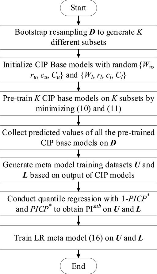
FIGURE 4. Flowchart of the proposed CIPE model training.
First, K different equal-sized subsets are generated by bootstrap resampling. Hyper-parameters of each base model are randomly assigned, and all base models are pre-trained on the corresponding subsets. In each CIP model, the optimal global solutions of minimizing (10) and (11) are the roots of their gradients Gu(∙) and Gl(∙) in (17) and (18), respectively. The trust-region algorithm (Zhang and Ordóñez, 2012) is chosen to search the root of Gu(∙) and Gl(∙). The proper gradient norm tolerance is set as the termination criteria.
After pre-training all base models, the original training dataset D is utilized for each pre-trained CIP base model to generate PI. The corresponding predicted upper and lower bounds of each CIP base model are separately collected to generate the meta model training datasets U and L, in which predicted bounds of base models are served as features. The quantile regression with proportion pair 1-PICP* and PICP* are conducted to obtain the sub-interval PIsub. Two LR meta models for the upper and lower bound are simultaneously trained through the MIP based on PIsub.
In the prediction process, the samples in the prediction dataset are first predicted by each CIP base model. K datasets of predicted upper and lower bounds are constructed. After that, the predicted upper and lower bounds of the PIs are separately combined by the two trained LR models to form the final upper and lower bounds of PI.
Compared with the single CIP model, the novel CIPE model avoids artificially determining the optimal value of the eight hyper-parameters of the biased convex cost function in the huge searching space. The integration of bagging and stacking improves the generalization performance and ensures the prediction accuracy and simplifies overall complexity.
In this section, to evaluate the performance of the proposed CIPE model, five other state-of-the-art interval prediction methods are employed for benchmarking. First, two other ensemble forecasting approaches, including CIP with a bagging ensemble (CIP-b) model and quantile regression forest (QRF) (Meinshausen, 2006), are utilized to confirm the ensemble performance. Second, two other methods concerning cost functions are used to examine the quality of the biased convex cost function, which are the bi-level optimization (BLO) (Safari et al., 2019)-based interval prediction model and LSTM with a gradient descend algorithm (LGD) (Li et al., 2020b)-based interval prediction model. Third, the CIP model is compared with CIPE to verify the improvement on model performance of the proposed method.
In the CIP-b model, PI is constructed by averaging the predicted upper and lower bounds of CIP base models which are utilized in CIPE. In the QRF model, a random forests algorithm regarded as the ensemble method is introduced to build PIs through calculating quantiles corresponding to the upper and lower bounds. In the BLO model, two independent ELMs are served as prediction engines and an even power polynomial function is proposed as the cost function. The hyper-parameters are tuned by the meta-heuristic algorithm. In the LGD model, a novel cost function applicable to the gradient descend algorithm is introduced into the deep learning network–based interval prediction model. LSTM with fully connected neural networks is employed as the prediction engine. In the CIP model, the hyper-parameters of the cost function are determined using the grid search method. All experiments are executed on a PC with an AMD 3600X CPU at 3.8 GHz CPU and 16 GB RAM.
The realistic wind farm data from Huashishan Wind Farm in Ningxia, China, are collected, which covers the period of time from June to August 2016 with 10-min resolution. The historical wind speed, wind direction, temperature, and calendar data are selected as the input features. Multi-horizon prediction experiments are implemented. The input vector and the prediction target are normalized to [0, 1] linearly by min-max scaling, respectively.
The proposed CIPE model has three hyper-parameters requiring manual setting, the number of base models K is set as 5, the number of hidden neurons of ELM in the base model is selected as 200, and the regularization coefficient in the MIP problem is set as 0.001. The parameters of the biased cost function are randomly assigned, as shown in Table 1. Two cost functions corresponding to upper and lower bounds have the same random rule, and the parameters remain unchanged during the training process. In BLO, the number of hidden neurons of ELM is set as 200 and the degree of the polynomial is 4. Particle swarm optimization (PSO) (Kennedy and Eberhart, 1995) is utilized to tune the hyper-parameters. In LGD, the hyper-parameter settings are mainly based on the work of (Li et al., 2020b) and artificially fine-tuned. In QRF, the number of trees, maximum depth of trees, and minimum size of leaf nodes are set as 200, 15, and 25, respectively. In CIP, the number of hidden neurons of ELM is also set as 200. The first 2/3 of samples are selected as the training dataset and the rest are the test dataset. All the approaches are compared based on the same datasets.
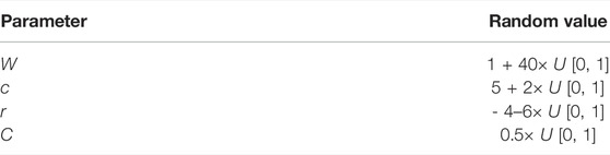
TABLE 1. Random generation rule of hyper-parameters of the biased cost function in CIPE.
In this study, the expected nominal coverage probability, PINC, in the test dataset is set as 90% and 95%. Since the deviation of PICP from PINC is inevitable, the average coverage deviation (ACD) is introduced to evaluate the performance of PIs in (19). The parameters η1 and η2 of CWC in (3) are set as 6 and 10, respectively.
The prediction results of various ensemble models in multi-step ahead prediction under different PINC are demonstrated in Table 2. It is evident that the proposed CIPE obtains better performance than QRF and CIP-b, and CIP-b behaves the worst. First, in the aspect of PICP, the evaluation index ACD indicates the compliance and volatility of PICP. Apparently, PICP of CIP-b significantly fluctuates and is severely substandard in most cases. CIPE and QRF have roughly the same reliability in PICP, but the variance for ACD of CIPE is equal to 0.076, which is smaller than that of QRF, 0.102, which means CIPE has better prediction stability. Second, in terms of PINAW, ignoring CIP-b for its poor performance in PICP, QRF tends to generate conservative intervals with the larger PINAW. Third, CWC comprehensively evaluates the quality of the constructed PIs. CIPE obtains the smallest value of CWC in most instances, further indicating that CIPE has comprehensive advantages in model performance.
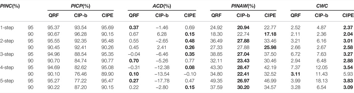
TABLE 2. Multi-step ahead prediction results of QRF, CIP-b, and CIPE under different PINC.
In the QRF model, the random forest structure is applied as the ensemble structure, and the quantile regression is regarded as the base predictor. In Table 2, CIPE obtains smaller PINAW than QRF in all the cases and is approximately 2% narrower than QRF, which means that the proposed CIPE is capable of constructing PI with better interval width under a similar coverage performance compared to QRF. Besides, except for the 4-step ahead prediction under PINC = 90%, in which CIPE produces substandard PICP, all values of index CWC of CIPE are smaller than those of QRF, demonstrating better ensemble performance of CIPE than QRF.
The intervals predicted by CIPE and QRF under PINC = 90% in 4-step ahead prediction and under PINC = 95% in 1-step ahead prediction are exhibited in Figure 5 and Figure 6, respectively. In Figure 5, PI constructed by CIPE is generally bracketed by and narrower than the one corresponding to QRF most of the time. The real targets tend to fall in the middle of the interval generated by CIPE, presenting its more reliable performance in prediction. In Figure 6, although the gap between two intervals is not quite obvious, the interval width of CIPE is still smaller than that of QRF at all times. During the period of high volatility marked by the red dotted box in Figure 6, the interval of QRF tends to guarantee PICP through generating spikes to increase the interval width. Therefore, CIPE has better performance in sharpness under similar reliability.
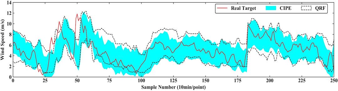
FIGURE 5. Prediction result of CIPE and QRF under PINC = 90% in 4-step ahead prediction.
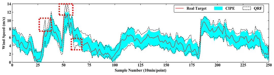
FIGURE 6. Prediction result of CIPE and QRF under PINC = 95% in 1-step ahead prediction.
CIP-b utilizes simple averaging to integrate the CIP base models used by CIPE. The prediction results of 5 different base models, CIP-b, and CIPE under PINC = 90% in multi-step ahead prediction are demonstrated in Table 3. It is evident that CIP-b suffers from large deviation around PINC and the greatest occurs in 4-step ahead prediction. In this circumstance, PINAW cannot reasonably describe the model performance of CIP-b because too high or too low PICP results in inappropriate interval width. Accordingly, the serious inadequacy of PICP exhibits bad prediction performance of CIP-b. This is because the simple averaging ensemble method of bagging proposes high requirement on the number of base models, and the serious shortage of base models is to blame for the performance of CIP-b. However, the proposed CIPE model effectively solves this problem through introducing the stacking ensemble approach.

TABLE 3. Multi-step ahead prediction results of different base models, CIP-b, and CIPE under PINC = 90%.
As long as the performance of all the base models is not too bad, CIPE can achieve a preferable and stable performance and has the capability of accommodating and ameliorating the bad performance of its base models. In 3-step ahead prediction of Table 3, it clearly observed that Base 1, Base 3, and Base 4 have severely substandard PICP, which are around 60%. In this case, CIPE can still construct PI which satisfies the coverage requirement. Moreover, CIPE can balance the narrow width caused by the substandard coverage rate and the wide width caused by the relatively high coverage rate. Similarly, in 4-step ahead prediction, the PICP of four base models scatter around 60%, while only one of them achieves above-standard performance. It is evident that PI constructed by CIPE still manifests relatively satisfying PICP which is close to PINC and preferable PINAW. It implies that CIPE mitigates the requirement of the number of base models and improves prediction performance.
Table 4 presents the prediction results of various models with uniquely designed cost function in multi-step ahead prediction under PINC = 90%. CIPE obtains the best performance among the three methods, demonstrating the superiority of its cost function. BLO utilizes a heuristic algorithm to find the optimal hyper-parameters, and the performance is seriously limited by the search space, maximum iterations, and other factors which are difficult to decide. Furthermore, the even power polynomial cost function pays much attention to PICP and ignores its balance with PINAW. Therefore, BLO tends to achieve substandard PICP, conservative PINAW, and unsatisfactory training efficiency. Besides, LGD employs two functions respectively corresponding to PICP and PINAW to form a cost function. However, the coverage part of the cost function leads to the possibility of interval crossover, posing great challenge to hyper-parameter adjustment. The average absolute ACD of LGD, which is equal to 0.53, is higher than that of CIPE, 0.35. It indicates that the performance of CIPE in PICP is closer to expectation than LGD. In terms of PINAW, the average improvement of CIPE compared to LGD is 19.56% and the maximum reaches 27.6%, which occurs in 1-step ahead prediction. From the perspective of the comprehensive index CWC, CIPE generally obtains the smallest value, which illustrates its preferable performance and further exhibits the superiority of the biased convex cost function.
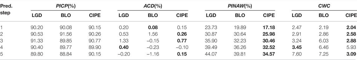
TABLE 4. Multi-step ahead prediction results of LGD, BLO, and CIPE under PINC = 90%.
Figure 7 and Figure 8 graphically present the specific comparisons of the prediction result. Figure 7 shows the prediction result of CIPE and BLO under PINC = 90% in 2-step ahead prediction. Generally, PI of CIPE is completely surrounded by that of BLO and the gap is clearly visible, indicating the better sharpness of the PI predicted by CIPE. Figure 8 presents the comparison between CIPE and LGD under PINC = 90% in 3-step ahead prediction. The result demonstrates that LGD tends to construct conservative PI with large interval width. It is evident that the boundaries of LGD prediction interval are relatively smooth, which cannot effectively reflect the characteristics of real targets. Therefore, the PI predicted by CIPE obtains better performance than those predicted by LGD and BLO.
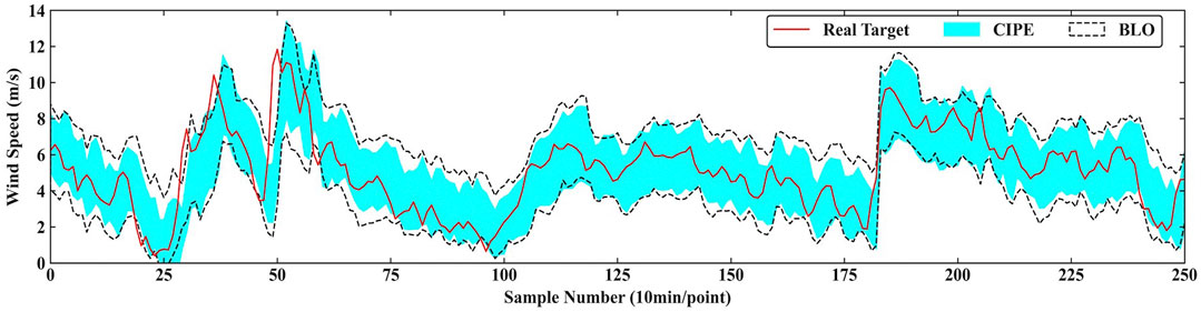
FIGURE 7. Prediction result of CIPE and BLO under PINC = 90% in 2-step ahead prediction.
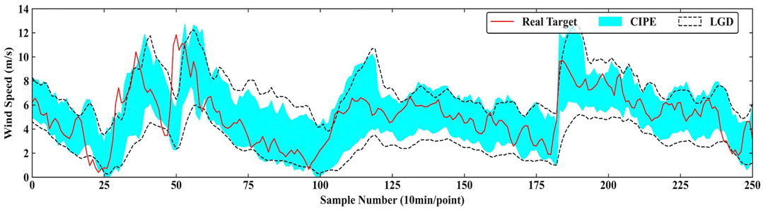
FIGURE 8. Prediction result of CIPE and LGD under PINC = 90% in 3-step ahead prediction.
The prediction results of CIP and CIPE under different PINC are presented in Table 5. CIPE generally has better performance than single CIP. In terms of ACD, the average absolute value of CIPE is equal to 0.35, which is smaller than that of CIP, 0.65. It implies CIPE possesses more preferable PICP performance which is closer to the expected coverage probability than single CIP. In the aspect of PINAW, CIPE obviously obtains narrower width than CIP in all cases and the average improvement reaches 7.48%. Besides, except for the 4-step ahead prediction under PINC = 90%, in which CIPE achieves substandard PICP, CIPE obtains smaller values of index CWC than CIP, demonstrating better comprehensive performance. Therefore, it illustrates that the prediction performance can be effectively improved through the proposed ensemble method.
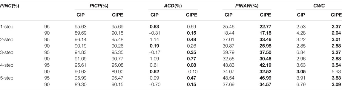
TABLE 5. Multi-step ahead prediction results of CIP and CIPE under different PINC.
Figure 9 and Figure 10 intuitively show the specific comparison of performance between CIPE and CIP under PINC = 90% in 2-step ahead prediction and under PINC = 95% in 1-step ahead prediction. It is clearly noticed that the upper bound of the interval generated by CIPE is significantly lower than that of the CIP model, while the lower bounds of the two models are very close. In Figure 9, the interval width of PI constructed by CIPE is about 3 m/s, and the gap compared to the one constructed by CIP is around 1 m/s. Figure 10 has a similar situation, which means that the CIP model tends to be more conservative in sharpness than the CIPE model.
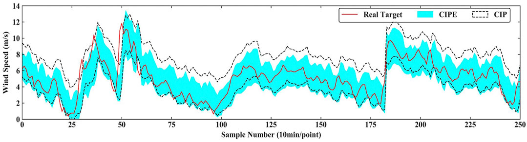
FIGURE 9. Prediction result of CIPE and CIP under PINC = 90% in 2-step ahead prediction.
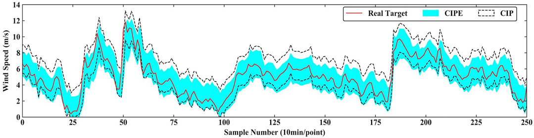
FIGURE 10. Prediction result of CIPE and CIP under PINC = 95% in 1-step ahead prediction.
The model training time under PINC = 90% is reported in Table 6. The model of CIP has the greatest computational cost due to the hyper-parameters’ searching by the grid search. The following is the BLO model because the training performance of the heuristic algorithm largely depends on the maximum number of iterations. The remaining four models have close computational times. The training time of CIP-b is the least owing to its simple averaging ensemble mechanism, but it suffers from unsatisfactory prediction performance. Except for CIP-b, the proposed CIPE method obtains the minimal training time. It illustrates that CIPE successfully alleviates the pressure of tuning hyper-parameters of the biased cost function and achieves superior training efficiency. In general, facilitated with the hybrid ensemble framework, the proposed CIPE model merits high potential for online model updating.
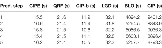
TABLE 6. Training time of different models under PINC = 90% in multi-step ahead prediction.
In this study, a CIP-based hybrid ensemble model for multi-horizon ahead wind speed interval prediction was proposed. The CIP model was a ELM predictor with a biased convex cost function based on LUBE prediction structure. To avoid the heavy training work of the CIP model, the ensemble technique was employed. The bagging and stacking ensemble methods were combined to aggregate multiple CIP models with randomly assigned hyper-parameters. The CIP models were trained first based on the sub-datasets generated using the bootstrap resampling technique of bagging ensemble. The LR model was chosen as the meta model to aggregate CIP base models instead of the average aggregation. The MIP method and quantile regression were utilized to train the hybrid ensemble model and determine the optimal parameters of the LR model. Due to the efficient computational performance of MIP and the biased convex cost function of CIP, the overall computational efficiency of CIPE is guaranteed, which is important for the short-term wind speed prediction. Comprehensive case studies under realistic wind farms validated the superior effectiveness and efficiency of the proposed CIPE model, exhibiting excellent PI quality and high potential for online application.
The raw data supporting the conclusions of this article will be made available by the authors, without undue reservation.
HL and CZ contributed to conception and design of the study. RG performed the statistical analysis and wrote the first draft of the manuscript. All authors contributed to manuscript revision and read and approved the submitted version.
This research was supported by the National Natural Science Foundation of China under Grant 51936003 and 51807023.
CZ was empolyed by Hangzhou Power Supply Company.
The remaining authors declare that the research was conducted in the absence of any commercial or financial relationships that could be construed as a potential conflict of interest.
All claims expressed in this article are solely those of the authors and do not necessarily represent those of their affiliated organizations, or those of the publisher, the editors, and the reviewers. Any product that may be evaluated in this article, or claim that may be made by its manufacturer, is not guaranteed or endorsed by the publisher.
Banik, A., Behera, C., Sarathkumar, T. V., and Goswami, A. K. (2020). Uncertain Wind Power Forecasting Using LSTM-Based Prediction Interval. IET Renew. Power Gener. 14 (14). doi:10.1049/iet-rpg.2019.1238
Hu, M., Hu, Z., Yue, J., Zhang, M., and Hu, M. (2017). A Novel Multi-Objective Optimal Approach for Wind Power Interval Prediction. Energies 10 (4). doi:10.3390/en10040419
Huang, G-B, Zhu, Q-Y, and Siew, C-K (2004). Extreme Learning Machine: a New Learning Scheme of Feedforward Neural Networks. Budapest, Hungary: IEEE International Joint Conference on Neural Networks, 2. 985–999.
Kennedy, J., and Eberhart, R., “Particle Swarm Optimization,” in IEEE International Conference on Neural Networks - Conference Proceedings, vol. 4, 1995.
Kavousi-Fard, A., Khosravi, A., and Nahavandi, S. (2016). A New Fuzzy-Based Combined Prediction Interval for Wind Power Forecasting. IEEE Trans. Power Syst. 31 (1)18-26. doi:10.1109/tpwrs.2015.2393880
Khosravi, A., Nahavandi, S., Creighton, D., and Atiya, A. F. (2011). Lower Upper Bound Estimation Method for Construction of Neural Network-Based Prediction Intervals. IEEE Trans. Neural Netw. 22 (3), 337–346. doi:10.1109/TNN.2010.2096824
Koenker, R., and Bassett, G. (1978). Regression Quantiles. Econometrica 46 (1)33. doi:10.2307/1913643
Li, C., Tang, G., Xue, X., Chen, X., Wang, R., and Zhang, C. 2020. The Short-Term Interval Prediction of Wind Power Using the Deep Learning Model with Gradient Descend Optimization. Renew. Energy 155, 197-211. doi:10.1016/j.renene.2020.03.098
Li, C., Tang, G., Xue, X., Saeed, A., and Hu, X. (2020). Short-Term Wind Speed Interval Prediction Based on Ensemble GRU Model. IEEE Trans. Sustain. Energy 11 (3)1370-1380. doi:10.1109/tste.2019.2926147
Li, H., Deng, J., Feng, P., Pu, C., and Arachchige, D. D. 2021. Short-Term Nacelle Orientation Forecasting Using Bilinear Transformation and ICEEMDAN Framework. Front. Energy Res. 9. doi:10.3389/fenrg.2021.780928
Li, H., Deng, J., Yuan, S., Feng, P., and Arachchige, D. D. 2021. Monitoring and Identifying Wind Turbine Generator Bearing Faults Using Deep Belief Network and EWMA Control Charts. Front. Energy Res. 9. doi:10.3389/fenrg.2021.799039
Li, H. 2022. SCADA Data Based Wind Power Interval Prediction Using LUBE-Based Deep Residual Networks. Front. Energy Res. 10. doi:10.3389/fenrg.2022.920837
Li, H. 2022. Short-Term Wind Power Prediction via Spatial Temporal Analysis and Deep Residual Networks. Front. Energy Res. 10. doi:10.3389/fenrg.2022.920407
Liu, F., Li, C., Xu, Y., Tang, G., and Xie, Y. (2020). A New Lower and Upper Bound Estimation Model Using Gradient Descend Training Method for Wind Speed Interval Prediction. Wind Energy 24(3):290-304. doi:10.1002/we.2574
Liu, W., and Xu, Y. (2020). Randomised Learning-Based Hybrid Ensemble Model for Probabilistic Forecasting of PV Power Generation. IET Gener. Transm. Distrib. 14 (24). doi:10.1049/iet-gtd.2020.0625
Long, H., Zhang, C., Geng, R., Wu, Z., and Gu, W. (2021). A Combination Interval Prediction Model Based on Biased Convex Cost Function and Auto Encoder in Solar Power Prediction. IEEE Trans. Sustain. Energy. doi:10.1109/tste.2021.3054125
Massaoudi, M., Refaat, S. S., Chihi, I., Trabelsi, M., Oueslati, F. S., and Abu-Rub, H. 2021. A Novel Stacked Generalization Ensemble-Based Hybrid LGBM-XGB-MLP Model for Short-Term Load Forecasting. Energy 214, 118874. doi:10.1016/j.energy.2020.118874
Moon, J., Jung, S., Rew, J., Rho, S., and Hwang, E. (2020). Combination of Short-Term Load Forecasting Models Based on a Stacking Ensemble Approach. Energy Build. 216 109921. doi:10.1016/j.enbuild.2020.109921
Safari, N., Mazhari, S. M., and Chung, C. Y. (2019). Very Short-Term Wind Power Prediction Interval Framework via Bi-level Optimization and Novel Convex Cost Function. IEEE Trans. Power Syst. 34 (2)1289-1300. doi:10.1109/tpwrs.2018.2872822
Shi, Z., Liang, H., and Dinavahi, V. (2018). Direct Interval Forecast of Uncertain Wind Power Based on Recurrent Neural Networks. IEEE Trans. Sustain. Energy 9 (3)1177-1187. doi:10.1109/tste.2017.2774195
Shrivastava, N. A., Lohia, K., and Panigrahi, B. K. (2016). A Multiobjective Framework for Wind Speed Prediction Interval Forecasts. Renew. Energy 87 903-910. doi:10.1016/j.renene.2015.08.038
Wan, C., Lin, J., Wang, J., Song, Y., and Dong, Z. Y. (2017). Direct Quantile Regression for Nonparametric Probabilistic Forecasting of Wind Power Generation. IEEE Trans. Power Syst. 32 (4), 2767-2778. doi:10.1109/tpwrs.2016.2625101
Wan, C., Wang, J., Lin, J., Song, Y., and Dong, Z. Y. (2018). Nonparametric Prediction Intervals of Wind Power via Linear Programming. IEEE Trans. Power Syst. 33 (1), 1074-1076. doi:10.1109/tpwrs.2017.2716658
Wan, C., Xu, Z., Pinson, P., Dong, Z. Y., and Wong, K. P. (2014). Optimal Prediction Intervals of Wind Power Generation. IEEE Trans. Power Syst. 29 (3), 1166-1174. doi:10.1109/tpwrs.2013.2288100
Wang, R., Li, C., Fu, W., and Tang, G. (2020). Deep Learning Method Based on Gated Recurrent Unit and Variational Mode Decomposition for Short-Term Wind Power Interval Prediction. IEEE Trans. Neural Netw. Learn Syst. 31 (10), 3814–3827. doi:10.1109/TNNLS.2019.2946414
Wolpert, D. H. (1992). Stacked Generalization. Neural Netw. 5 (2), 241-259. doi:10.1016/s0893-6080(05)80023-1
Xiyun, Y., Xue, M., Guo, F., Huang, Z., and Jianhua, Z. (20172017). Wind Power Probability Interval Prediction Based on Bootstrap Quantile Regression Method. CAC. Proceedings - 2017 Chinese Automation Congress, 2017-January. doi:10.1109/cac.2017.8243005
Zhang, C., and Ordóñez, R. (2012). Numerical Optimization. Advances in Industrial Control, 9781447122234. doi:10.1007/978-1-4471-2224-1_2
Zhang, Y., Zhao, Y., Pan, G., and Zhang, J. (2020). Wind Speed Interval Prediction Based on Lorenz Disturbance Distribution. IEEE Trans. Sustain. Energy 11 (2), 807-816. doi:10.1109/tste.2019.2907699
Keywords: interval prediction, wind speed prediction, biased convex cost function, ensemble learning, mixed integer programming
Citation: Long H, Geng R and Zhang C (2022) Wind Speed Interval Prediction Based on the Hybrid Ensemble Model With Biased Convex Cost Function. Front. Energy Res. 10:954274. doi: 10.3389/fenrg.2022.954274
Received: 27 May 2022; Accepted: 13 June 2022;
Published: 15 July 2022.
Edited by:
Long Wang, University of Science and Technology Beijing, ChinaReviewed by:
Yusen He, Grinnell College, United StatesCopyright © 2022 Long, Geng and Zhang. This is an open-access article distributed under the terms of the Creative Commons Attribution License (CC BY). The use, distribution or reproduction in other forums is permitted, provided the original author(s) and the copyright owner(s) are credited and that the original publication in this journal is cited, in accordance with accepted academic practice. No use, distribution or reproduction is permitted which does not comply with these terms.
*Correspondence: Huan Long, aGxvbmdAc2V1LmVkdS5jbg==
Disclaimer: All claims expressed in this article are solely those of the authors and do not necessarily represent those of their affiliated organizations, or those of the publisher, the editors and the reviewers. Any product that may be evaluated in this article or claim that may be made by its manufacturer is not guaranteed or endorsed by the publisher.
Research integrity at Frontiers
Learn more about the work of our research integrity team to safeguard the quality of each article we publish.