 Zhiyu Wang
 Zhen Zhu
 Geyang Xiao
 Bing Bai
- Intelligent Network Research Institute, Zhejiang Lab, Hangzhou, China
Energy load forecasting is a critical component of energy system scheduling and optimization. This method, which is classified as a time-series forecasting method, uses prior features as inputs to forecast future energy loads. Unlike a traditional single-target scenario, an integrated energy system has a hierarchy of many correlated energy consumption entities as prediction targets. Existing data-driven approaches typically interpret entity indexes as suggestive features, which fail to adequately represent interrelationships among entities. This paper, therefore, proposes a neural network model named Cross-entity Temporal Fusion Transformer (CETFT) that leverages a cross-entity attention mechanism to model inter-entity correlations. The enhanced attention module is capable of mapping the relationships among entities within a time window and informing the decoder about which entity in the encoder to concentrate on. In order to reduce the computational complexity, shared variable selection networks are adapted to extract features from different entities. A data set obtained from 13 buildings on a university campus is used as a case study to verify the performance of the proposed approach. Compared to the comparative methods, the proposed model achieves the smallest error on most horizons and buildings. Furthermore, variable importance, temporal correlations, building relationships, and time-series patterns in data are analyzed with the attention mechanism and variable selection networks, therefore the rich interpretability of the model is verified.
1 Introduction
The integrated energy system (IES) is regarded as one of the most important forms of modern energy systems (Tahir et al., 2021). A comprehensively optimized IES is capable of delivering considerable energy savings, pollution reduction advantages, better system stability, etc. (Zhang et al., 2020; Wang et al., 2022). One key specification of IES is the demand pattern of the energy end-users. Therefore, demand forecasting can provide insights to enhance system design, scheduling strategy, and control optimization for IES (Dittmer et al., 2021).
Statistic and machine learning techniques have long been applied for the demand forecasting of end-users. The former techniques are straightforward strategies that focus on the target time series’ statistics. The latter techniques are trained with a period of load data accompanied with auxiliary information before making predictions based on recent data. Typical statistic models include thesimple linear regression model, moving average (MA) strategy, and autoregression (AR) algorithm. Auto-Regressive Integrated Moving Average (ARIMA) is a combination of MA and AR, which includes stationary stochastic variables in the non-stationary stochastic process. As a result, it is capable of reproducing time series patterns (Newsham and Birt, 2010). Notable traditional machine learning methods include Partial Least Squares Regression (PLSR), Ridge Regression (RR), and Support Vector Regression (SVR). PLSR basically uses the covariance between the input and output variables instead of analyzing the hyperplanes with the least variance between the dependent and independent variables (Hosseinpour et al., 2016). In RR models, a shrinkage estimator is added to the diagonal elements of the correlation matrix (Sun et al., 2019). SVR leverages kernel functions for modeling the nonlinear transformation. These models often ignore the chronological order of variables and struggle to properly model the temporal features in the data.
Time-series forecasting approaches based on deep learning have significantly grown in recent years, with the development in neural network algorithms, available data, and hardware power. Recurrent neural networks (RNN) (Rumelhart and McClelland, 1987) is a category of neural network suitable for time-series modeling. RNNs use hidden states that are iteratively supplied back to the network for temporary time-related information representation and storage, as implied by the name (Tang et al., 2021). This gives the model memory for temporal properties. However, RNN suffers from the vanishing gradient problem (Ribeiro et al., 2020). The hidden state will gradually degrade during simulation for long-term sequences. To alleviate this problem, improved implementation of RNN including Long Short-Term Memory (LSTM) (Hochreiter and Schmidhuber, 1997) and GRU Gated Recurrent Unit (GRU) (Chung et al., 2014) have been proposed. These networks introduce a gate for controlling time-series information. The gates assist the network in selecting critical data that requires long-term memory. As a result, both networks can make predictions for extended periods of time before the vanishing gradient problem appears Ayodeji et al. (2022).
The Transformer (Vaswani et al., 2017), which employs an attention mechanism to describe cross-time interactions for time series, has recently become one of the most popular network architectures. The attention module accepts all time frame inputs and provides weights that directly map the impact of the previous time frame on future targets. Therefore, the gradient vanishing problem due to long-time dependence is eliminated. Another benefit of the transformer is that the network grants better interpretability. Natural language processing (Tetko et al., 2020) and computer vision (Dosovitskiy et al., 2021), two of the most important domains of artificial intelligence, have both benefited greatly from the transformer. The better modeling capabilities of this model, however, come at the cost of more computation. The computational complexity of attention to explicitly simulate the cross-time relationship is O (n2), where n is the scale of time frames. In comparison, the computational complexity of most neural network implementations, such as GRU and LSTM, is O(n). Meanwhile, while the transformer solves the problem of time dependence, it does not support input selection inside a single time frame.
Combining LSTM and Transformer, the Temporal Fusion Transformer (TFT) proposed by Lim et al. (2021) is a state-of-the-time model for multi-horizon forecasting. TFT leverages a backbone network based on LSTM layers for variable selection and encoding. The attention module receives the output from LSTM at all time frames as input, which addresses LSTM’s disadvantage by efficiently modeling time dependence.
For time-series forecasting including multiple entities, the TFT uses entity encodings to distinguish entities and independent networks to produce predictions, without modeling the correlation between entities. As a result, TFT may not cope well with the correlation among entities across different time steps, which is crucial for IES load forecasting (Feng and Zhang, 2020; Wang R. et al., 2021).
Therefore, the Cross-Entity Temporal Fusion Transformer (CETFT) was developed in this research as an improved version of the Transformer structure geared to energy load forecasting with correlations across distinct entities. The cross-entity attention module and entity encoding networks based on shared variable selection blocks are two innovative methods offered to adapt the network to multi-entity prediction tasks. This allows for simultaneous quantification of correlation across entities and time domains. Experiments on 13 buildings on a university campus are conducted to compare the proposed method to existing predicting algorithms. Future analyses are taken to comprehensively evaluate the interpretability of the network, Including cross-time correlations, cross-entity correlations, special attention to unconventional time-series trends, and variable importance.
The remaining of this paper is organized as follows: Section 2 gives an introduction and mathematical definition of IES and time series forecasting; In Section 3, the structure of the proposed CETFT and its submodules are explained in detail; Section 4 carried out a case study based on the campus building data set evaluating the performance and interpretability of the proposed model; and Section 5 briefly concludes this paper.
2 Preliminary
2.1 Integrated Energy Systems
The IES is mainly composed of multiple energy supply, exchange, storage, and consumption entities (Lin and Fang, 2019). These entities could transmit energy to each other according to a certain scheduling strategy to achieve a balance within the system and minimize the overall energy usage and expense. One major concern in achieving this goal is forecasting loads of consumption entities in advance, and the interdependence of entities is critical to achieving this goal.
2.2 Time-Series Forecasting
As illustrated in Figure 1, the goal of load forecasting can be framed as a supervised learning problem on time-series data. The data are a sequence of observations with equal time intervals, including targets and auxiliary information. The object of the problem is to forecast future target values based on historical data.
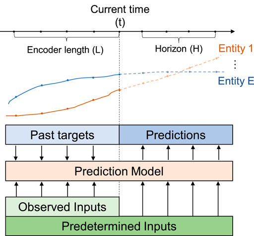
FIGURE 1. Demonstration of a time-series forecasting problem with multiple entities.
These data are organized in chronological order and grouped into a series of time windows of equal lengths. Each time window is further divided into two parts by a given forecast time frame t. In the inference phase, it is typically sufficient to take as input data a short period before the prediction time to encode the current state. The length of the data window as inputs is denoted by L. Those after the forecast time are outputs of the problem. The forecasting horizon is given by H, which is the number of time frames to be forecast.
In an IES, there are typically multiple entities that are correlated to each other. Let E be the number of unique entities in the system, e.g., different buildings on a campus, indexed by 1, 2, … , E. The target is the energy load
From the perspective of accessibility, the features χt = [ut; xt] are divided into known features that can be predetermined ahead of time (e.g., calendar features) and unknown features ut that are observed and must be predicted for future values (e.g., meteorological information). Typically, the targets are also a subset of the unknown features. The features χi associated with a certain entity i include the private property of that entity and public features that affect the entire area.
The object of the problem is to construct a model f (⋅) to forecast future outputs for each entity in a time period, which is denoted by:
where f (⋅) is the proposed prediction model. The output
3 Methodology
The basic idea of neural networks is to apply weights to inputs through serial layers, in the form of:
where
The weights are hard parameters that only change during learning and are insistent during inferences. In contrast, recently developed neural networks tend to utilize “soft” weights to simulate the cognitive attention to inputs, of which a typical example is the attention mechanism (Vaswani et al., 2017). These networks leverage additional branch layers to adaptively calculate weights from inputs, which are again multiplied by the inputs at the layer at the main route.
The proposed CETFT utilizes two of these modules. First is the cross-entity attention module, which builds associations between each entity at different times. The second is the variable selection network (Lim et al., 2021) used for entity encoding, which simulates the importance of features for understanding the state of each entity at each time. In this paper, both these modules have been improved to adapt to the cross-entity situation. This section will provide a detailed definition of these two key modules and also the overall architecture of the network.
3.1 CETFT Architecture
The CETFT can be roughly separated into three sequential submodules, as shown in Figure 2: 1) the cross-entity attention, 2) the entity encoding network, and 3) the output layers. Gated residual networks are used to connect adjacent sub-modules and further process intermediate variables. These modules will be defined in this section.
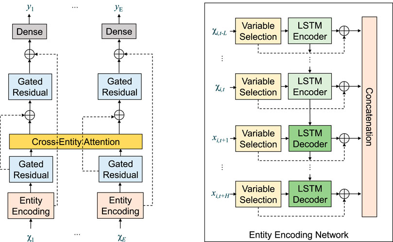
FIGURE 2. CETFT architecture. Entity encoding networks receive inputs directly related to theirs corresponding entity, and the outputs are concatenated chronologically. The cross-entity attention integrates information from all entities and time frames. Gated residual layers provide enhancement to skip connections. Dense layers generate forecasting results.
3.2 Cross-Entity Attention
In order to model the correlation among entities as well as time steps at the same forecast time, A cross-entity attention mechanism is employed for the temporal fusion transformer. The attention module receives encoded vectors from entity encoding networks and generates temporally enhanced feature vectors for the output layer. Before the module, an encoded vector of dinput will be generated for all entities from all times. For a system with E entities, L encoder length, and H decoder length, the number of vectors available is E (L + H). The attention module receives two matrics as input:
where
where exp (⋅) is the power with natural base. The output of the whole module is with dimension EH × dv.
The process can be interpreted as a weighted sum of the features. The weights are calculated by multiplying the keys from all time and queries within the prediction horizon. The module scale the feature vectors according to the relationship among time frames and scale the input according to the estimated attention.
For time series forecasting, a decoding mask M should be applied to define the causal relationships between embeddings (Li et al., 2019). The encoding embeddings, however, are available to all time frames. Therefore, the mask for a single-entity attention mask is shaped like a right-angled trapezoid. The lengths of the top base and the bottom base are equal to the size of encoder embeddings and the size of all embeddings, respectively. The mask is described as a matrix
The mask matrix is illustrated in the left sub-figure in Figure 3.
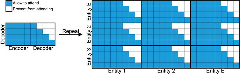
FIGURE 3. Left: The original self-attention mask for TFT. Right: The cross-entity attention mask for CETFT, generated by repeating the single-entity attention mask by E times both horizontally and vertically.
To adapt to a multiple-entity application, the attention mask should be repeated by the number of entities both horizontally and vertically, which is illustrated in Figure 3. Mathematically, the cross-entity mask is defined as:
Furthermore, to increase the representative capability of the attention mechanism, it is common to stack multiple attention heads into a multi-head attention module, which is defined as:
where h is the index of attention head, mh is the number of heads, and
3.3 Entity Encoding Networks
The entity encoding modules are a set of networks for producing encoded vectors from raw inputs, which are passed to the attention layer. The network consists of two components in series. Firstly, the shared variable selection network filters important variables in the input, and then the LSTM layers will initially extract the time information.
3.3.1 Shared Variable Selection
At different times, the variables that have the main impact on the forecast are different. The variable selection networks are intended to screen valuable variables and apply weights to those variables based on their projected importance.
The inputs will be categorized according to distinct entities initially, as indicated in Figure 2. Each input will be sent into a single variable selection network at each time frame. All of these networks’ outputs will be collected and organized in the same hierarchy as their inputs.
Before being fed into the networks, the numerical inputs are normalized. The categorical inputs will be encoded using a normalized vector whose length is determined by the number of available values. After this process, it makes no difference to the network whether the input is continuous or discrete, except that discrete variables are represented as a vector rather than a single value. Without loss of generality, the following definition will be based on a single continuous variable.
In practice, the variable selection network modules can be reused if the same features are shared across time or entities, which is similar to how the modules were shared for encoders and decoders in the original TFT model. Different from the original TFT implementation, the variable selection networks are shared among entities to reduce the complexity of the network. These networks rely on the idea of a Gated Residual Network (GRN) defined by Lim et al. (2021) as follows:
where ω is an identifier of the network that corresponds to a certain input element, LayerNorm is a standard layer normalizer by Ba et al. (2016), and η1,
The Gated Linear Unit (GLU) is (Dauphin et al., 2017):
where σ(⋅) is the sigmoid function and ⊙ is Hadamard product, W3,ω. W4,ω, b3,ω, b4,ω are learnable layer parameters.
In practice, individual shared variable selection networks are built for each element in the model input. Let χj,t be j-th normalized or encoded input variable at time frame t, the variable selection layer is:
where
On the other hand, the input χj,t is handled by an extra GRN layer associated with itself:
Individual variable selection networks corresponding to the inputs connected with a certain entity are collected based on pre-defined entity attributes, and their outputs are aggregated into a single vector. Let
Note that aside from inside the entity encoding networks, the GRN blocks also act as connectors of the main modules in the CETFT network.
3.3.2 LSTM Layers
LSTM layers are a type of RNN layers that receive inputs of the current time and also hidden inputs from past time. The mathematical definition of LSTM can be found in the paper by Hochreiter and Schmidhuber (1997). The LSTM layers generate two parts of return values, namely the output vector and the hidden vector. The output vector, as indicated by the name, is the variable passed to other modules. On the other hand, the hidden vector is passed back to the layer.
In CETFT, the LSTM layers are used to further process the features of each time output by the variable selection network to initially extract the time information. The past inputs
3.4 Output Layer
The outputs of the attention module will pass through another GRN before a set of dense layers are introduced to generate quantile outputs for the model. The model will generate multiple outputs corresponding to the forecasted values of each entity at each prediction time. In addition, the quantile loss by Sharda et al. (2021) summed across all outputs is used to train CETFT.
4 Case Study
4.1 Dataset and Evaluation Setting
The data set is a collection of energy loads of 13 buildings at the University of Texas at Dallas, accompanied by 21 columns of auxiliary variables including meteorological records and calendar information1. The recordings span from January 2014 to December 2015 with a 1-h sample interval, providing a total of 17,520 records.
The buildings can be separated into six categories, as listed in Table 1. B9 is a site equipped with photovoltaic panels, whose load drops to negative numbers during the daytime. B2 is a lecture hall. Its load is relatively small and drops to 0 about 30% of the time. All other buildings have higher loads during the day and lower loads at night, but their load patterns vary with different categories. The correlations among these buildings can be clearly seen from Pearson analysis illustrated in Figure 4. A list of auxiliary features and their accessibility and types are shown in Table 2. The correlations among meteorological variables are illustrated in Figure 5. The heat map indicates high correlations among the variables related to irradiance and temperature, while they share a negative correlation with the solar zenith angle and relative humidity.
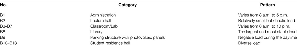
TABLE 1. Building categories and energy load patterns.
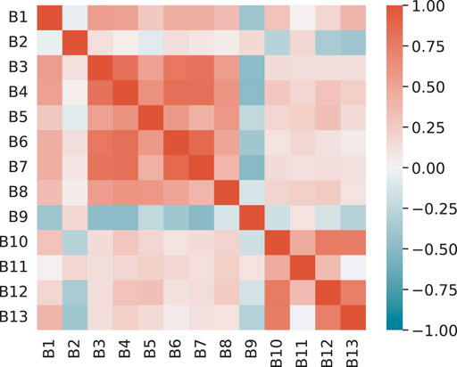
FIGURE 4. Pearson correlation of building loads.
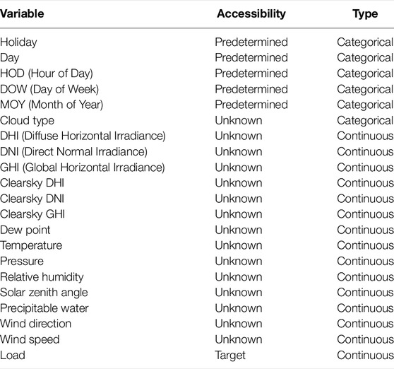
TABLE 2. Feature and target specification in the UTD dataset.
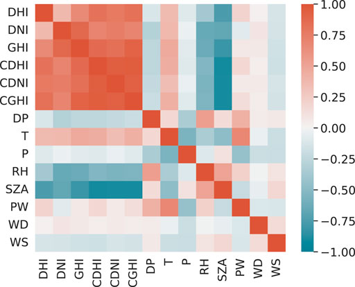
FIGURE 5. Pearson correlation of meteorological variables. CDHI, clearsky DHI; CDNI, clearsky DNI; CGHI, clearsky GHI; DP, dew point; T, temperature; P, pressure; RH, relative humidity; SZA, solar zenith angle; PW, precipitable water; WD, wind direction; WS, wind speed.
The categorical inputs are converted to encoding vectors, while continuous inputs are normalized. These inputs are concatenated into a vector for each entity at each time step. The data sets are chronologically divided into training/validation/test sets with a ratio of 0.7:0.15:0.15. The forecast horizons are selected as 1, 6, 12, and 24 h ahead. This horizon configuration is based on the daily periodicity of the time series and is commonly adopted by recent works (Arsov et al., 2021; He et al., 2022). In the test data set, there are 1460 and 846 missing data of buildings B2 and B9 out of 2628 records, respectively, and therefore the two buildings are excluded from forecast targets during model evaluation.
The hyperparameters CETFT and TFT are tuned with the Optuna framework (Akiba et al., 2019). The range of the hyperparameters are: network layer size range in [8, 256], attention head size in [1, 16], learning rate range in [1e-5, 0.1], dropout range in [0.1, 0.3]. The model is optimized based on the loss on the evaluation set, and the optimized model is further evaluated on the test set. The Ranger optimizer is adopted for training, with the batch size equal to 128 and a max epoch of 300. The learning rate is divided by 10 if the evaluation loss has stopped reducing for 4 epochs, and the training will early stop after 10 epochs without performance improvement.
The models to be compared are roughly divided into three categories: identification-based methods, of which a representative algorithm ARIMA; traditional statistical methods, including PLSR, RR and SVR; and deep-learning-based methods, including LSTM, GRU and TFT. The metric used for evaluation is Symmetric Mean Absolute Percentage Error (sMPAE) which is commonly used in time-series forecasting in the field of energy (Demir et al., 2021; Meira et al., 2021; Putz et al., 2021):
where n is the amount of prediction made. A smaller value of the metric indicates a better performance of the model.
4.2 Comparison With Baseline
Table 3 collects the sMAPE error of all testing scenarios, covering different horizons, models, and buildings. The best model is marked in bold in each line. It can be seen that CETFT has achieved the best performance in 37 tests out of 44. The remaining best results were achieved by TFT, RR, and ARIMA, respectively. From an architectural point of view, CETFT achieves the best results for all horizons with the exception of B1, B5, and B8. In terms of computational complexity, our network takes 3 h and 27 min to train, while TFT takes 1 h and 25 min on an Nvidia A100 GPU with 40 GiB memory.
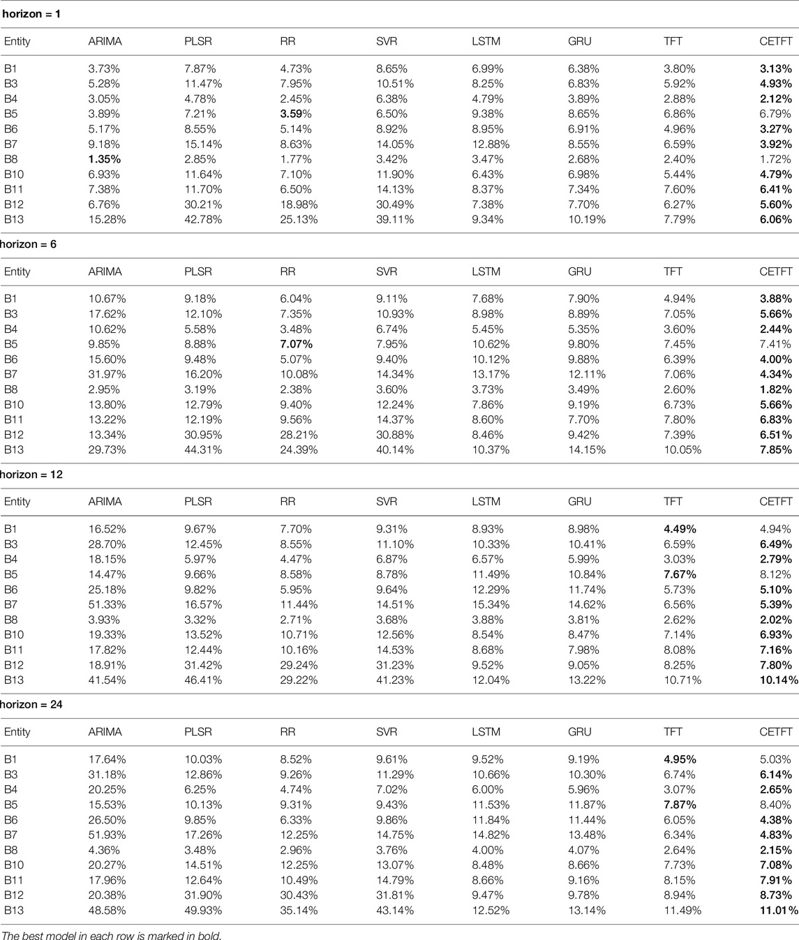
TABLE 3. SMAPE on the UTD dataset.
All models’ predictive power declines as the horizon lengthen, which is to be expected given the limited amount of information available for future forecasts. ARIMA is the model that suffers the most as the horizon lengthens. Although ARIMA performed best on B8 when horizon = 1, it quickly became the model with the biggest error as the horizon was extended. When the horizon is increased from 12 to 24, however, the ARIMA error does not greatly rise, which can be explained by the cyclical pattern of energy usage throughout the day.
Statistical machine learning models including PLSR, RR, and SVR have obtained similar results. The RR model’s accuracy gradually drops as the horizon lengthens, whereas PLSR and SVR remain reasonably stable. When horizon = 1, however, the latter two already have bigger errors. As a result, the RR model has a superior overall performance. There is a more remarkable phenomenon regarding these models, that is, their performance on buildings B12 and B13 is rather poor. These statistical models may fail to capture special patterns related to certain entities in the time series, resulting in inaccurate forecasts.
LSTM and GRU, the two RNN-based models, have relatively similar model performance. The accuracy of these two models is relatively little influenced by the prediction horizon. These two models outperform statistical machine learning techniques for B10–B13 prediction, but they don’t have any evident advantages in other buildings. In general, neither of these two models may be particularly favorable for multi-entity forecasting.
The TFT is the closest to the proposed CETFT in terms of performance. But on most buildings, especially buildings including B6 and B7, CETFT still shows a clear advantage, where the error is reduced by about 1–2 percentage points. When the horizon is smaller, CETFT offers more visible advantages than TFT. This reflects CETFT’s superiority over TFT in extracting information from entities. In general, CETFT delivers the best overall forecasting performance by combining the advantages of TFT for time-series forecasting with advances based on multi-entity forecasting.
4.3 Model Interpretability
It is feasible to interpret the model by examining the runtime weights during prediction thanks to the incorporation of two soft-weight-based network structures, namely the cross-entity attention module and shared variable selection network. Both of these networks will assign bigger weights to the more important inputs each time the model makes a prediction (Ding et al., 2020; Niu et al., 2021). As a result, a probabilistic assessment of the contribution or importance of a particular object (i.e., a variable/entity/time frame) to the prediction can be made by aggregating the soft weights pertaining to that object across the whole data set (Lim et al., 2021).
Several use cases, including 1) variable importance assessment, 2) cross-entity relationship evaluation, 3) cross-time relationship evaluation, and 4) time-series pattern identification, will be exhibited in this section to evaluate the model’s interpretability.
4.3.1 Variable Importance Assessment
By aggregating the weights of the shared variable selection networks, it is possible to assess the importance of different variables to the network. The importance of all variables and known variables can be determined by aggregating the weights of the variable selection network in the encoder and decoder sections, respectively. The two classes of importance are normalized so that their sum is equal to 1, and the result is recorded in Tables 4, 5. In these two tables, the importance percentages greater than 5% and 10% are, respectively marked in bold, indicating key variables for encoding and decoding.
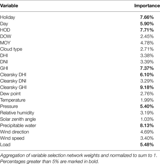
TABLE 4. Importance of variable importance for past inputs.
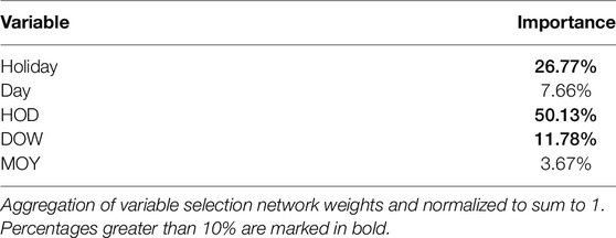
TABLE 5. Importance of variable importance for future inputs.
Holiday, day, HOD, GHI, clearsky DHI, clearsky GHI, Pressure, precipitable water, and load are critical factors in the encoder stage, according to the model. Because the load has a clear daily periodicity and is considerably affected by holidays, the impact of holidays and hours on the forecast is interpretable. The variables related to sunlight are strongly correlated, and the importance of clearsky GHI is the highest for all variables, but some of the variables are of low importance. This could be because the variable selection network identifies redundant features and reduces dimensionality. It is worth noting that the importance of the load itself is not at its peak. This illustrates the importance of auxiliary variables in load forecasting.
On the decoder side, Holidays and hours still have a very important impact on the prediction. However, the rank of date and DOW is the opposite of those of the encoder. This may be due to the fact that the information of DOW is partially contained in the Day variable, and the network decreases the dimensionality of the two and retains the influence of one of the variables for the same reason as the sunlight-related variables.
4.3.2 Cross-Entity Relationship Evaluation
The cross-entity relationship is evaluated by aggregating and normalizing the weights of the attention module per entity, as illustrated in Figure 6. The figure maps the normalized attention from different buildings to predicate to the encoded feature vectors of different buildings. High, medium, and low attention are indicated by the colors red, white, and green, respectively. Note that the attention is not necessarily synced with correlation, as the former more likely represents the model’s assessment of causality between variables (Wang X. et al., 2021; Yang et al., 2021).
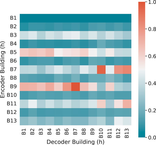
FIGURE 6. Heatmap of attention weights aggregated per entity. The horizontal axis represents the entity being input, and the vertical axis denoted the entity being predicted.
It can be seen that B9 has received the most attention from other buildings. This makes sense because B9 has photovoltaic panels installed, which is the only building with electricity generating capacity, and its energy consumption pattern differs significantly from the others. Higher weights are given to three classroom/lab buildings (B3, B5, and B7), as well as two student living halls (B11, B13). This reflects the model’s selection of variables with a similar pattern. The administration building (B1), the lecture hall (B2), and the library (B8) are three structures that are reasonably independent or utilize a consistent amount of energy. As a result, their contribution to the prediction is minor.
4.3.3 Cross-Time Relationship Evaluation
Similar to the cross-entity relationship, it is also possible to identify the cross-time relationship by aggregating the attention weights per time. The heatmap is shown as Figure 7. This relationship is expressed in relative time rather than absolute time, and the axis tick tables represent hours relative to the current time.
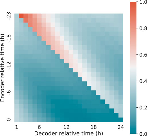
FIGURE 7. Heatmap of attention weights aggregated per time. The horizontal axis represents the entity being input, and the vertical axis denoted the entity being predicted.
A diagonal line running from the upper left to the lower right is clearly visible in the figure. This shows that the network is mostly interested in information from the same hour the day before. Each time frame’s attention in the encoder peaks right of the diagonal line, then gradually decreases and again increases in chronological order. This is primarily owing to the variable’s periodic character. The majority of inputs of interests occur at the same time the day before, as well as a few hours ahead of the prediction time.
This figure also demonstrates the difficulty in long-term series forecasting. While the attention mechanism can directly model correlations across time frames, the amount of attention the network can provide diminishes over time. Maximum attention is given to the first prediction, while the attention level becomes increasingly distracted over time. As a result, longer-period projections are still insufficiently informative and perform poorly.
4.3.4 Time-Series Pattern Identification
Attention weights can also be aggregated in terms of absolute time frames. This allows time-series pattern identification by providing a picture of how much each actual time frame contributes to the model output.
Figure 8 uses the attention provided at different past times collected from building B4, B5, B6, and B12 for demonstration of this capability of the network. The horizontal axis represents the number of hours elapsed since Sunday, 13 September 2015, which is the first day in the test data set. The load of B6 is shown in red, while the overall attention is shown in cyan. It can be seen that loads of the four buildings all show obvious periodic characteristics within a cycle of 24 h. For B4, B5, and B6, the loads show consistent behavior during workdays, but a different pattern occurs each weekend. The first such change occurs at about 100 h. Therefore, there is also a cyclical feature with a period of a week (i.e., 168 h). Simultaneously, the network’s attention has shown a similar periodicity, with a notable spike over the weekend. The time-series pattern for B12 is a bit different. The load for B12 does not show a clear periodicity based on weeks. Instead, the load generally shows an upward trend over time. Corresponding to this characteristic, the attention to B12 experienced a rise when the load dropped. These analyses demonstrate how the attention module reacts to the input time-series patterns and pays particular attention to particular changes. This provides insight for automatic analysis of the time-series characteristics and significant events.
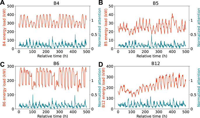
FIGURE 8. Load and normalized attention to building (A) B4, (B) B5, (C) B6, and (D) B12 for 500 h since 13 September 2015.
5 Conclusion
This paper presents a deep-learning-based model named CETFT for multi-entity energy load forecasting. Entity encoding networks and a cross-entity attention module are defined. In a case study involving 13 buildings on a university campus, the proposed model achieves the minimum errors on all buildings given different prediction horizons. Further analyses are performed to assess the model’s interpretability, revealing the relevance of variables, linkages between entities and time frames, and time-series features. The concept of selection networks could be used in future work to address the complexity of cross-entity attention processes and strike a balance between model correctness and computation overhead, along with improved fine-grained input categories for better adaption to a wider variety of time-series data.
Data Availability Statement
The original contributions presented in the study are included in the article/supplementary material, further inquiries can be directed to the corresponding author.
Author Contributions
ZW and ZZ developed the CETFT model and implement the computer code and wrote the initial draft, GX revised and edited the draft. BB validated the experiments and results, YZ prepared visualization and data presentation.
Funding
This work is supported by Key Research Project of Zhejiang Lab (No. 2021LE0AC02).
Conflict of Interest
The authors declare that the research was conducted in the absence of any commercial or financial relationships that could be construed as a potential conflict of interest.
Publisher’s Note
All claims expressed in this article are solely those of the authors and do not necessarily represent those of their affiliated organizations, or those of the publisher, the editors, and the reviewers. Any product that may be evaluated in this article, or claim that may be made by its manufacturer, is not guaranteed or endorsed by the publisher.
Footnotes
1The data is accessible on the website of IEEE Data Port (https://dx.doi.org/10.21227/jdw5-z996).
References
Akiba, T., Sano, S., Yanase, T., Ohta, T., and Koyama, M. (2019). “Optuna,” in Proceedings of the ACM SIGKDD International Conference on Knowledge Discovery and Data Mining, 2623–2631. doi:10.1145/3292500.3330701
Arsov, M., Zdravevski, E., Lameski, P., Corizzo, R., Koteli, N., Gramatikov, S., et al. (2021). Multi-horizon Air Pollution Forecasting with Deep Neural Networks. Sensors 21, 1–18. doi:10.3390/s21041235
Ayodeji, A., Wang, Z., Wang, W., Qin, W., Yang, C., Xu, S., et al. (2022). Causal Augmented ConvNet: A Temporal Memory Dilated Convolution Model for Long-Sequence Time Series Prediction. ISA Trans. 123, 200–217. doi:10.1016/j.isatra.2021.05.026
Ba, J. L., Kiros, J. R., and Hinton, G. E. (2016). “Layer Normalization,” in 4th International Conference on Learning Representations, ICLR 2016 - Conference Track Proceedings. doi:10.48550/arXiv.1607.06450
Chung, J., Gulcehre, C., Cho, K., and Bengio, Y. (2014). “Empirical Evaluation of Gated Recurrent Neural Networks on Sequence Modeling,” in NIPS 2014 Workshop on Deep Learning, 1–9. doi:10.48550/arXiv.1412.3555
Clevert, D. A., Unterthiner, T., and Hochreiter, S. (2016). “Fast and Accurate Deep Network Learning by Exponential Linear Units (ELUs),” in 4th International Conference on Learning Representations, ICLR 2016 - Conference Track Proceedings. doi:10.48550/arXiv.1511.07289
Dauphin, Y. N., Fan, A., Auli, M., and Grangier, D. (2017). “Language Modeling with Gated Convolutional Networks,” in 34th International Conference on Machine Learning, ICML 2017, 1551–1559. 2. doi:10.48550/arXiv.1612.08083
Demir, S., Mincev, K., Kok, K., and Paterakis, N. G. (2021). Data Augmentation for Time Series Regression: Applying Transformations, Autoencoders and Adversarial Networks to Electricity Price Forecasting. Appl. Energy 304, 117695. doi:10.1016/j.apenergy.2021.117695
Ding, Y., Zhu, Y., Feng, J., Zhang, P., and Cheng, Z. (2020). Interpretable Spatio-Temporal Attention LSTM Model for Flood Forecasting. Neurocomputing 403, 348–359. doi:10.1016/j.neucom.2020.04.110
Dittmer, C., Krümpel, J., and Lemmer, A. (2021). Power Demand Forecasting for Demand-Driven Energy Production with Biogas Plants. Renew. Energy 163, 1871–1877. doi:10.1016/j.renene.2020.10.099
Dosovitskiy, A., Beyer, L., Kolesnikov, A., Weissenborn, D., Zhai, X., Unterthiner, T., et al. (2021). “An Image Is Worth 16x16 Words: Transformers for Image Recognition at Scale,” in International Conference on Learning Representations, 1–22. doi:10.48550/arXiv.2010.11929
Feng, C., and Zhang, J. (2020). Assessment of Aggregation Strategies for Machine-Learning Based Short-Term Load Forecasting. Electr. Power Syst. Res. 184, 106304. doi:10.1016/j.epsr.2020.106304
He, X., Shi, S., Geng, X., and Xu, L. (2022). Information-aware Attention Dynamic Synergetic Network for Multivariate Time Series Long-Term Forecasting. Neurocomputing 500, 143–154. doi:10.1016/j.neucom.2022.04.124
Hochreiter, S., and Schmidhuber, J. (1997). Long Short-Term Memory. Neural Comput. 9, 1735–1780. doi:10.1162/neco.1997.9.8.1735
Hosseinpour, S., Aghbashlo, M., Tabatabaei, M., and Khalife, E. (2016). Exact Estimation of Biodiesel Cetane Number (Cn) from its Fatty Acid Methyl Esters (Fames) Profile Using Partial Least Square (Pls) Adapted by Artificial Neural Network (Ann). Energy Convers. Manag. 124, 389–398. doi:10.1016/j.enconman.2016.07.027
Li, S., Jin, X., Xuan, Y., Zhou, X., Chen, W., Wang, Y. X., et al. (2019). “Enhancing the Locality and Breaking the Memory Bottleneck of Transformer on Time Series Forecasting,” in Advances in Neural Information Processing Systems 32 (NeurIPS 2019).
Lim, B., Arık, S., Loeff, N., and Pfister, T. (2021). Temporal Fusion Transformers for Interpretable Multi-Horizon Time Series Forecasting. Int. J. Forecast. 37, 1748–1764. doi:10.1016/j.ijforecast.2021.03.012
Lin, R., and Fang, F. (2019). “Energy Management Method on Integrated Energy System Based on Multi-Agent Game,” in 2019 International Conference on Sensing, Diagnostics, Prognostics, and Control (SDPC), 564–570. doi:10.1109/SDPC.2019.00107
Meira, E., Cyrino Oliveira, F. L., and de Menezes, L. M. (2021). Point and Interval Forecasting of Electricity Supply via Pruned Ensembles. Energy 232. doi:10.1016/j.energy.2021.121009
Newsham, G. R., and Birt, B. J. (2010). “Building-level Occupancy Data to Improve ARIMA-Based Electricity Use Forecasts,” in BuildSys’10 - Proceedings of the 2nd ACM Workshop on Embedded Sensing Systems for Energy-Efficiency in Buildings, 13–18. doi:10.1145/1878431.1878435
Niu, Z., Zhong, G., and Yu, H. (2021). A Review on the Attention Mechanism of Deep Learning. Neurocomputing 452, 48–62. doi:10.1016/j.neucom.2021.03.091
Putz, D., Gumhalter, M., and Auer, H. (2021). A Novel Approach to Multi-Horizon Wind Power Forecasting Based on Deep Neural Architecture. Renew. Energy 178, 494–505. doi:10.1016/j.renene.2021.06.099
Ribeiro, A. H., Tiels, K., Aguirre, L. A., and Schön, T. (2020). “Beyond Exploding and Vanishing Gradients: Analysing Rnn Training Using Attractors and Smoothness,” in Proceedings of the Twenty Third International Conference on Artificial Intelligence and Statistics. Editors S. Chiappa, and R. Calandra, 108, 2370–2380. PMLR of Proceedings of Machine Learning Research.
Rumelhart, D. E., and McClelland, J. L. (1987). Learning Internal Representations by Error Propagation. MIT Press, 318–362.
Sharda, S., Singh, M., and Sharma, K. (2021). RSAM: Robust Self-Attention Based Multi-Horizon Model for Solar Irradiance Forecasting. IEEE Trans. Sustain. Energy 12, 1394–1405. doi:10.1109/TSTE.2020.3046098
Sun, M., Ghorbani, M., Chong, E. K., and Suryanarayanan, S. (2019). “A Comparison of Multiple Methods for Short-Term Load Forecasting,” in 51st North American Power Symposium, NAPS 2019. doi:10.1109/NAPS46351.2019.8999984
Tahir, M. F., Chen, H., and Han, G. (2021). A Comprehensive Review of 4E Analysis of Thermal Power Plants, Intermittent Renewable Energy and Integrated Energy Systems. Energy Rep. 7, 3517–3534. doi:10.1016/j.egyr.2021.06.006
Tang, Y., Yu, F., Pedrycz, W., Yang, X., Wang, J., and Liu, S. (2021). Building Trend Fuzzy Granulation Based LSTM Recurrent Neural Network for Long-Term Time Series Forecasting. IEEE Trans. Fuzzy Syst. 30, 1599–1613. doi:10.1109/TFUZZ.2021.3062723
Tetko, I. V., Karpov, P., Van Deursen, R., and Godin, G. (2020). State-of-the-art Augmented NLP Transformer Models for Direct and Single-step Retrosynthesis. Nat. Commun. 11. doi:10.1038/s41467-020-19266-y
Vaswani, A., Shazeer, N., Parmar, N., Uszkoreit, J., Jones, L., Gomez, A. N., et al. (2017). “Attention Is All You Need,” in Advances in Neural Information Processing Systems, 30. Long Beach, USA: NIPS 2017, 1–11.
Wang, R., Sun, Q., Sun, C., Zhang, H., Gui, Y., and Wang, P. (2021a). Vehicle-Vehicle Energy Interaction Converter of Electric Vehicles: A Disturbance Observer Based Sliding Mode Control Algorithm. IEEE Trans. Veh. Technol. 70, 9910–9921. doi:10.1109/TVT.2021.3105433
Wang, R., Sun, Q., Zhang, H., Liu, L., Gui, Y., and Wang, P. (2022). Stability-Oriented Minimum Switching/Sampling Frequency for Cyber-Physical Systems: Grid-Connected Inverters under Weak Grid. IEEE Trans. Circuits Syst. I Regul. Pap. 69, 946–955. doi:10.1109/TCSI.2021.3113772
Wang, X., Xu, X., Tong, W., Roberts, R., and Liu, Z. (2021b). InferBERT: A Transformer-Based Causal Inference Framework for Enhancing Pharmacovigilance. Front. Artif. Intell. 4, 1–11. doi:10.3389/frai.2021.659622
Yang, X., Zhang, H., Qi, G., and Cai, J. (2021). Causal Attention for Vision-Language Tasks, 9842–9852. doi:10.1109/CVPR46437.2021.00972
Zhang, D., Jianhua, B., Sun, X., and You, P. (2020). “Research on Operational Economics of the Integrated Energy System,” in 2020 4th International Conference on Power and Energy Engineering (ICPEE), 251–255. doi:10.1109/ICPEE51316.2020.9310986
Nomenclature
τ prediction time offset
χt initial input
ω shared variable selection network identifier
b layer bias
dinput input dimension
dlayer layer dimension
dk dimension of key
dv dimension of value
E number of entities
f(⋅) prediction model
H attention head
H prediction Horizon
i entity index
K key matrix
L encoder length
M attention mask matrix
mh number of attention head
n amount of predictions
Q query matrix
t time frame
tF end of future time window
tS starting time of input
ut observed input
V value matrix
v input identifier
W layer weight
xt predetermined input
yi actual target value
z layer input vector
Z layer input matrix
Keywords: integrated energy system, time-series forecasting, multi-entity forecasting, load forecasting, neural networks, transformer network
Citation: Wang Z, Zhu Z, Xiao G, Bai B and Zhang Y (2022) A Transformer-Based Multi-Entity Load Forecasting Method for Integrated Energy Systems. Front. Energy Res. 10:952420. doi: 10.3389/fenrg.2022.952420
Received: 25 May 2022; Accepted: 10 June 2022;
Published: 22 July 2022.
Edited by:
Qiuye Sun, Northeastern University, ChinaReviewed by:
Jingwei Hu, State Grid Liaoning Power Company Limited Economic Research Institute, ChinaTianyi Li, Aalborg University, Denmark
Ning Zhang, Anhui University, China
Copyright © 2022 Wang, Zhu, Xiao, Bai and Zhang. This is an open-access article distributed under the terms of the Creative Commons Attribution License (CC BY). The use, distribution or reproduction in other forums is permitted, provided the original author(s) and the copyright owner(s) are credited and that the original publication in this journal is cited, in accordance with accepted academic practice. No use, distribution or reproduction is permitted which does not comply with these terms.
*Correspondence: Geyang Xiao, eGd5YWxhbkBvdXRsb29rLmNvbQ==