 Zhao Liu
 Jiateng Li2
 Yanshun Zhao
95% of researchers rate our articles as excellent or good
Learn more about the work of our research integrity team to safeguard the quality of each article we publish.
Find out more
ORIGINAL RESEARCH article
Front. Energy Res., 13 July 2022
Sec. Smart Grids
Volume 10 - 2022 | https://doi.org/10.3389/fenrg.2022.947532
This article is part of the Research TopicAdvanced AI Applications for Modelling, Optimization, Control, and Planning of Smart GridView all 39 articles
The increasing penetration of renewable energy introduces more uncertainties and creates more fluctuations in power systems than ever before, which brings great challenges for automatic generation control (AGC). It is necessary for grid operators to develop an advanced AGC strategy to handle fluctuations and uncertainties. AGC dynamic optimization is a sequential decision problem that can be formulated as a discrete-time Markov decision process. Therefore, this article proposes a novel framework based on proximal policy optimization (PPO) reinforcement learning algorithm to optimize power regulation among each AGC generator in advance. Then, the detailed modeling process of reward functions and state and action space designing is presented. The application of the proposed PPO-based AGC dynamic optimization framework is simulated on a modified IEEE 39-bus system and compared with the classical proportional−integral (PI) control strategy and other reinforcement learning algorithms. The results of the case study show that the framework proposed in this article can make the frequency characteristic better satisfy the control performance standard (CPS) under the scenario of large fluctuations in power systems.
Automatic generation control (AGC) is applied to ensure frequency deviation and tie-line power deviation within the allowable range in power systems as a fundamental part of energy management system (EMS) (Jaleeli et al., 2002). Conventional AGC strategies calculate the total adjustment power based on the present information collected from Supervisory Control and Data Acquisition (SCADA) system including frequency deviation, tie-line power deviation, and area control error (ACE), etc., and then allocates the total adjustment to each AGC unit. The control period is generally 2–8 s. Therefore, the key to conventional AGC strategies is to solve two problems: ① how to calculate the total adjustment power based on the online information; ② how to allocate the total adjusted power to each AGC unit with the goal of satisfying the control performance standard (CPS) and minimizing the operation cost. At present, to solve these two problems, scholars have proposed many control strategies. For calculating the total adjustment power, proposed strategies include the classical proportional−integral (PI) control (Concordia and Kirchmayer, 1953), proportional−integral-derivative (PID) control (Sahu et al., 2015; Dahiya et al., 2016), optimal control (Bohn and Miniesy, 1972; Yamashita and Taniguchi, 1986; Elgerd and Fosha, 2007), adaptive control (Talaq and Al-Basri, 1999; Olmos et al., 2004), model predictive control (Atic et al., 2003; Mcnamara and Milano, 2017), robust control (Khodabakhshian and Edrisi, 2004; Pan and Das, 2016), variable structure control (Erschler et al., 1974; Sun, 2017), and intelligent control technologies such as neural network (Beaufays et al., 1994; Zeynelgil et al., 2002), fuzzy control (Talaq and Al-Basri, 1999; Feliachi and Rerkpreedapong, 2005), and genetic algorithm (Abdel-Magid and Dawoud, 1996; Chang et al., 1998). In terms of allocating total adjustment power to each AGC unit, a baseline allocation approach is proposed according to the adjustable capacity ratio and installed capacity ratio of each unit without considering the differences of dynamic characteristic among units. Additionally, Yu et al. (2011) treated the power allocation as a stochastic optimization problem, which can be discretized and modeled as a discrete-time Markov decision process. Also, the problem is solved by utilizing the Q-learning algorithm of reinforcement learning.
In general, the conventional AGC strategy is designed under a typical feedback-loop structure with the characteristic of hysteresis, which regulates the future output of AGC units based on the present input signal. However, the penetration of large-scale renewable energy introduces high stochastic disturbance to modern power grid due to the characteristic of dramatical fluctuation (Banakar et al., 2008). The phenomenon has not only increased regulation capacity of AGC units but also put forward higher requirement for coordinated control ability of generation units with different dynamic characteristics (such as thermal and hydroelectric units). Nevertheless, the fast regulation capacity of units in power systems is limited. When the load or renewable energy generations is continuously rising or falling, the units with second-level regulation performance will approach its upper or lower regulation limit. At this point, it is hard to ensure the frequency deviation and tie-line power deviation within an allowable range if the fast regulation capacities are insufficient in the system. On the other hand, the adjustment ratio of different units is different, i.e., to be exact, thermal units have minute-level regulation performance, while hydroelectric units have second-level regulation performance. Therefore, these strategies cannot effectively coordinate units with different characteristics, which will cause overshoot or under-adjustment. At present, the goal of AGC strategies is to maintain the dynamic control performance of system to comply with CPS established by the North American Electric Reliability Council (NERC) (Jaleeli and Vanslyck, 1999). CPS pays more attention to the medium- and long-term performance of system frequency deviation and tie-line power deviation, while it no longer requires the ACE to cross zero every 10 min and aims to smoothly regulate the frequency of power systems.
To address the hysteresis issues of conventional AGC strategies and make the dynamic performance satisfy CPS, some scholars put forward the concept of AGC dynamic optimization (Yan et al., 2012). The basic idea can be described as the optimization of the regulation power of AGC units in advance based on ultra-short-term load forecasting and renewable energy generation forecasting information, different security constraints, and objective functions. The strategy aims to optimize the AGC units’ regulation power in the next 15 min, and the optimization step is 1 min. From the perspective of dispatching framework formulated by the power grid dispatching center, the AGC dynamic optimization can be viewed as a link between real-time economic dispatch (especially for the next 15 min) and routine AGC (control period is 2–8 s), which can achieve a smooth transition between the two dispatch sections. Compared with economic dispatch, AGC dynamic optimization takes the system’s frequency deviation, tie-line power deviation, and ACE and CPS values into account. Compared with conventional AGC strategies, it introduces load and renewable energy forecasting information into account which can better handle renewable energy’s fluctuation. Moreover, the dispatch period is 1 min which adapts to the thermal AGC units with minute-level regulation characteristics.
Yan et al. (2012) proposed a mathematic model for AGC dynamic optimal control. It takes the optimal CPS1 index and minimizes ancillary service cost as objective function. The system constraints are considered including system power balance constraints, AGC units’ regulation characteristics, tie-line power deviation, and frequency deviation. This model added ultra-short-term load forecasting information into the power balance constraints as well as mapping the relationship between system frequency and tie-line power. Zhao et al. (2018) expanded the model proposed in Yan et al. (2012), taking the ultra-short-term wind power forecasting value and its uncertainties into account and conducted a chance constraint programming AGC dynamic optimization model with probability constraints and expected objectives. An optimal mileage-based AGC dispatch algorithm is proposed in Zhang et al. (2020). Zhang et al. (2021a) further extended the methods in Zhang et al. (2020) with adaptive distributed auction to handle the high participation of renewable energy. A novel random forest-assisted fast distributed auction-based algorithm is developed for coordinated control in large PV power plants in response to the AGC signals (Zhang et al., 2021b). A decentralized collaborative control framework of autonomous virtual generation tribe for solving the AGC dynamic dispatch problem was proposed in Zhang et al. (2016a).
In general, the existing research defined AGC dynamic optimal control as a multistage nonlinear optimization problem that includes objective functions and constraint conditions. To deal with the uncertainties of wind power, some scholars adopted chance-constrained programming method based on the probabilistic model of wind power. However, the accurate probability information of random variables is difficult to model, which limits the accuracy and practicality of this method. Moreover, the stochastic programming model is too complex to solve. Furthermore, these methods cannot take the future fluctuations of wind power into account when making decisions.
Artificial intelligence-based methods have been developed in recent years to address the AGC command dispatch problem, including the lifelong learning algorithm and the innovative combination of the consensus transfer of the Q learning (Zhang et al., 2016b; Zhang et al., 2018). Deep reinforcement learning (DRL) is a branch of machine learning algorithms and an important method of stochastic control based on the Markov decision process, which can better solve sequential decision problems (Sutton and Barto, 1998). Recently, DRL has been successfully implemented on many applications of power systems, such as optimal power flow (Zhang et al., 2021a), demand response (Wen et al., 2015), energy management system for microgrid (Venayagamoorthy et al., 2016), autonomous voltage control (Zhang et al., 2016b), and AGC (Zhou et al., 2020; Xi et al., 2021). In AGC problems, as stated previously, the presented literatures usually focus on the power allocation problem which still belongs to the conventional AGC strategy. Different from the previous works, this article focuses on AGC dynamic optimization and utilizes 1 minute time resolution wind power and loads forecasting values, which are collected from and used by real wind farms and grid dispatching centers, to regulate the power outputs of AGC units. Unlike the existing optimization model, this article defines AGC dynamic optimization as a Markov decision process and a stochastic control problem and takes the various uncertainties and fluctuations of wind power outputs into account. To better solve the dynamic optimization and support safe online operations, the proximal policy optimization (PPO) deep reinforcement learning algorithm is implemented, with the clipping mechanism of PPO, which can provide more reliable outputs (Schulman et al., 2015).
The key contributions of this article are summarized as follows: ① by formulating the AGC dynamic optimization problem as the Markov decision process with appropriate power grid simulation environment, reasonable state space, action space, and reward functions, the PPO-DRL agent can be trained to learn how to determine the regulation power of AGC units without violating the operation constraints; ② by adopting the state-of-the-art PPO algorithm (Wang et al., 2020), the well-trained PPO-DRL agent could consider the uncertainties of wind power fluctuations in the future when making decisions at the current moment.
The remaining parts of this article are organized as follows: Introduction provides the advanced AGC dynamic optimization model considering wind power integration and the details of how to transform advanced AGC dynamic optimization into a multistage decision problem. Introduction introduces the principles of reinforcement learning, PPO algorithm, and the procedures of the proposed methodology. In Introduction, the IEEE 39-bus system is utilized to demonstrate the effectiveness of the proposed method. Finally, some conclusions are given in Introduction.
The essential strategy of AGC dynamic optimization is an advanced control strategy, which aims to optimize the adjustment power of each AGC unit per minute in the next 15 min according to the ultra-short-term load and wind generation forecasting information as well as the current operation condition of each unit, system frequency, and tie-line power. The objective function is to minimize the total adjustment cost, while the system dynamic performance (i.e., frequency, tie-line power deviation, and ACE) is to comply with CPS and satisfy the security constraints. Specifically, the constraints include system power balance, CPS1 and CPS2 indicators, frequency deviation, tie-line power deviation limit, and AGC unit regulation characteristics. The mathematical model of AGC dynamic optimization is formulated as follows:
where
1) Power balance constraints:
where
2) CPS1 constraints:
where
where
3) CPS2 constraints:
where
4) Power output constraints of units:
where
5) Ramp power constraints of units:
where
6) Tie-line power deviation constraints:
where
7) Frequency deviation constraints:
where
A reinforcement learning framework includes an agent and an environment, as illustrated in Figure 1, which aims at maximizing a long-term reward through abundant interactions between the agent and the environment. At each step t, the agent observes states
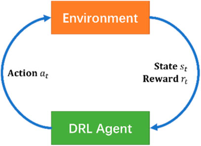
FIGURE 1. Environment–DRL agent interaction loop of reinforcement learning.
The interaction between the agent and environment can be modeled by a Markov decision process, which is a standard mathematical formalism of sequential decision problems. A typical Markov decision is denoted by a tuple
The policy is a rule used by an agent to decide what actions to take, which maps the action from a given state. A stochastic policy is usually expressed as
The state value functions
The action-value function
The advantage function
In general, the DRL algorithms can be divided into the value-based, the policy-based, and the actor-to-critic (A2C) framework. The proximal policy optimization (PPO) algorithm follows the A2C framework with an actor network and a critic network.
The main advantage of applying PPO algorithm to the AGC optimization problem is that the new control action decision updates from the policy network does not change too much from the previous policy and can be restrained within the feasible region by the clipping mechanism. During the off-line training process, the PPO also converges faster than other DRL algorithms. Also, during the on-line operations, the PPO generates smoother, less variance, and more predictable sequential decisions, which is desired for the AGC optimization.
The overall structure of the PPO algorithm is presented in Figure 2, including an actor network and a critic network. The AGC training environment sends the experience tuples
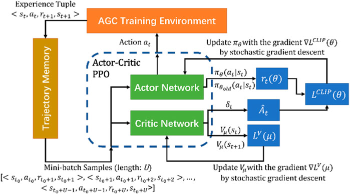
FIGURE 2. Structure of PPO algorithm.
The actor network and the critic network are realized by deep neural networks (DNNs) with the following equations:
where
The actor network contains the policy model
The conventional policy gradient-based DRL optimizes the following objective function (Wang et al., 2020):
where
where
where
The input of the actor network is the observation state
where
The importance sampling and clipping function help the PPO DRL algorithm achieve better stability and reliability for AGC online operations, better data efficiency and computation efficiency, and better overall performance.
If the regulation power of each AGC unit is regarded as the action of the agent and the real power system is regarded as the environment of the agent, then the AGC dynamic optimization model considering the uncertainty of wind power can be transformed into a typical random sequential decision problem. Combining the description of the aforementioned AGC dynamic optimization mathematical model, the 15-min control cycle can be divided into a 15-stage Markov process. The framework is shown in Figure 3.
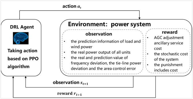
FIGURE 3. Framework of grid environment interacting with an agent.
The agent can be trained offline through historical data and massive simulations and then applied online in the real power grid. This section mainly focuses on the efficient offline training process of such agent, which introduces the design of several important components.
State space S: the setting of the state space should consider the factors that may affect the decision as much as possible. In this work, the state space is determined as a vector of system information representing the current system condition at time t and prediction system information at time
Action space A: action space is the decision variable in the optimization model, including the ramp direction and ramp power. In this article, to avoid the lack of generality, the action is defined as power increments of AGC units
The design of reward function is crucial in DRL. It generates reward
where the cost term
where
Here, the real power deviations
where
The power output of any unit (AGC or non-AGC unit) relates to the frequency deviation, tie-line power deviation, and ACE. Taking an interconnection power grid of two areas as an example, the system contains region A and region B. The control strategy of the two areas is the tie-line bias frequency control. It is assumed that
Frequency deviation, tie-line power deviation, and area control error can be calculated as follows:
where B is the equivalent frequency regulation constant for the control area in MW/0.1Hz and the value is negative.
The punishment term
The AGC units participate in both primary and secondary frequency control; thus, the outputs of AGC units at time
where
Accordingly, the power outputs of non-AGC units at time
The outputs of AGC and non-AGC units are subjected to the corresponding maximum and minimum power limits:
where
where
The following two functions denote the frequency deviation and tie-line power transfer deviation punishments, respectively:
where
In this article, we added an additional performance evaluation term
State transition probability P: in this work, the reinforcement learning algorithm based on the model-free method is utilized, so the state of the agent at the next time and rewards can be obtained by the interaction with the environment, and they make up state transition probability P including environmental stochasticity.
Discount factor
Based on the aforementioned analysis, this article transforms the AGC dynamic optimization problem into a sequential decision issue and utilizes the PPO deep reinforcement learning algorithm to solve the proposed problem. The AGC dynamic optimization problem based on the PPO algorithm is shown in Figure 4. The specific process is described as follows:
1) Initialize the weight and bias of the neural network, actor and critic neural network learning rate, reward discount factor
2) Initialize the initial observation value at the first moment from the power system environment.
3) Input state observation
4) Implement action
5) Input
6) Update the actor and critic neural network models according to
7) Repeat steps 2–6 until the number of training episodes is equal to the set number M.
8) Save the parameters of actor and critic neural networks. Utilize the trained agent on the test data.
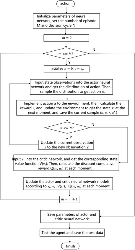
FIGURE 4. AGC dynamic optimization problem based on the PPO algorithm.
In this article, the PPO agent for AGC dynamic optimization control is tested on the modified IEEE 39 bus system model which includes three AGC units and seven non-AGC units. The tie-line is connected to bus 29, and a wind farm with 130 MW installations is connected to bus 39. A single-line diagram of the system is shown in Figure 5.
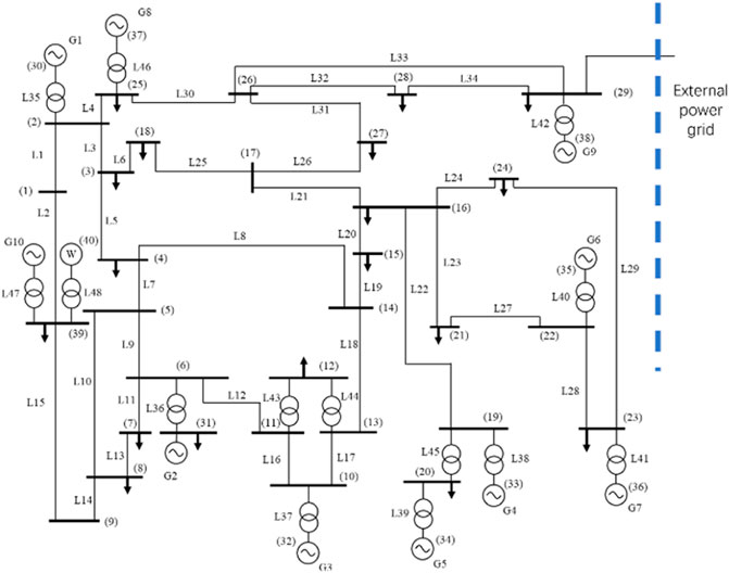
FIGURE 5. Modified IEEE 39 bus system.
The forecasting and actual data of load and wind power come from New England power grid1. The basic parameters of three AGC units and test system are shown in Tables 1, 2. The control period is set at 15 min, and it is assumed that the deviation of frequency and tie-line transmission power at the initial time are 0.
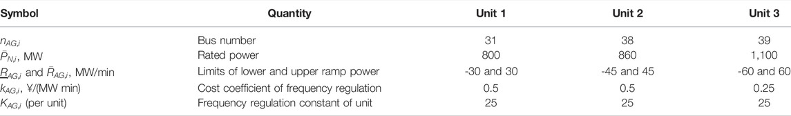
TABLE 1. Information of AGC units.
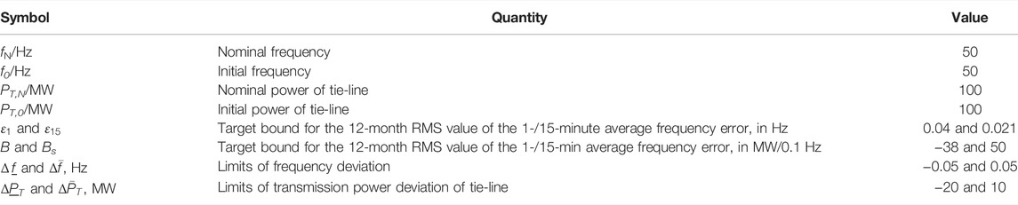
TABLE 2. Information of the test system.
The action space refers to the regulation power of AGC units at each optimization moment, which is determined by ramp power limits of each AGC unit. The per unit action space of the three AGC units is set as follows:
In addition, the state space dimension is 35 according to the preceding description, which includes information on 19 forecasting loads at time t+1, actual output power of 10 units at time t, and actual and forecasting values of system frequency deviation, transmission power deviation, and ACE separately at time t and t+1. The dimensions of state space and action space, respectively, correspond to the neural numbers of input and output layers. Therefore, this work sets up three hidden layers both in actor and critic neural networks, and the number of neurons in each layer is 64, 128, and 32, respectively. The activation function in each hidden layer is the ReLU function. A larger learning rate
Based on the preceding model and significant parameters, the PPO agent is coded using the TensorFlow framework with Python 3.7. The results of CPS1 index are shown in Figure 6.
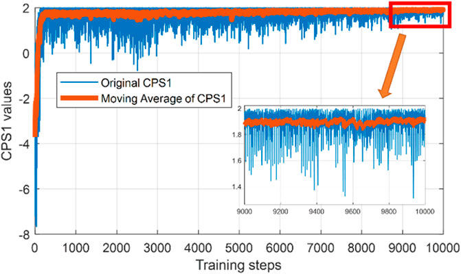
FIGURE 6. Results of CPS1 index in the training process using 10,000 episodes.
The x-axis represents the number of episodes being trained, while the y-axis represents the value of CPS1 index in each episode. It can be observed that the CPS1 values of the first few hundreds of episodes are relatively low and unstable. As training episodes increase, CPS1 values are kept within a stable range around 191.3%, which fits CPS. In comparison, the deep Q learning (DQL) algorithm and the duel deep Q learning (DDQL) algorithm are also implemented. The average CPS1 values are 187.4 and 184.5%. This shows that the PPO architecture for AGC unit dynamic optimization proposed in this article can effectively learn the growing uncertainties in the power system. Once the agent is trained, it can make proper decisions based on its trained strategy combined with environmental observation data feedback. Specifically, the agent trained in this work receives data from the power system, including actual information of unit output power, frequency, tie-line transmission power, ACE, and forecasting information of load, wind power, frequency, tie-line transmission power, and ACE as its observation, and then makes decisions for the regulation power of AGC units at time t, that is, advanced control of AGC units, in order to reduce the frequency deviation at time t+1.
In addition, taking a typical control period of the system as an example, Figure 7 shows the actual load, the wind power generations, and the net load by subtracting the wind generations from the actual load. The load at each bus is allotted in proportion to the load of the original IEEE-39 node system.
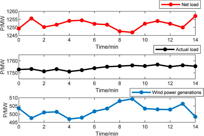
FIGURE 7. Curve of load with wind power fluctuations.
Using PI hysteresis control and PPO algorithm for frequency control in this period, the results of system frequency deviation, transmission power deviation of tie-line, and ACE are represented in Figures 8A–C, respectively.
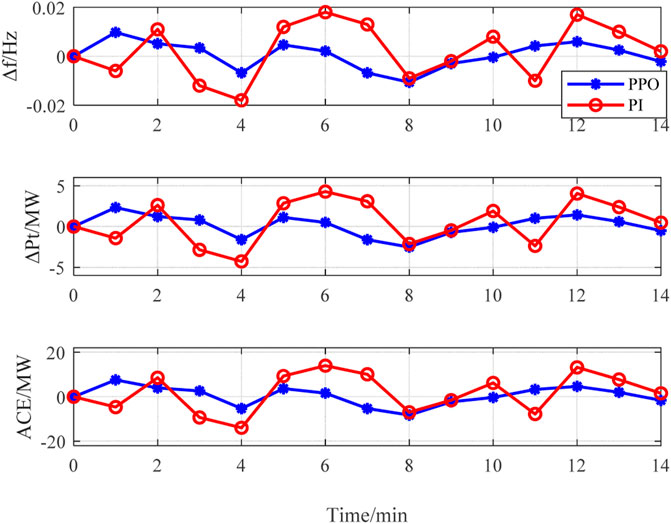
FIGURE 8. Results of the optimization method and PPO algorithm.
It is observed in Figure 8A that the outputs of both the PPO agent and optimization method can meet the requirements of frequency deviation (i.e., ±0.05 Hz). Moreover, maximum frequency deviation of the system controlled by the PPO agent is 0.0175 Hz, which is superior to -0.044 Hz that is controlled by the optimization method. This demonstrated that the dynamic optimization strategy of AGC units based on PPO algorithm is able to mitigate the frequency fluctuation of the system efficiently by advanced control of AGC units.
Figure 8B shows the transmission power deviation of tie-line. The power deviation under the optimization method is relatively large, which contains three times the off-limit conditions owing to the AGC resources in the system that are insufficient. While under PPO agent controller, the power deviation fluctuation is smaller without over-limit time. It proves that the system operation is more stable when using the PPO agent controller optimization method. In addition, as shown in Figure 8C, the agent performs much better than the optimization method when calculating the values of ACE. Figure 9 shows the AGC power regulation curve of all AGC units.
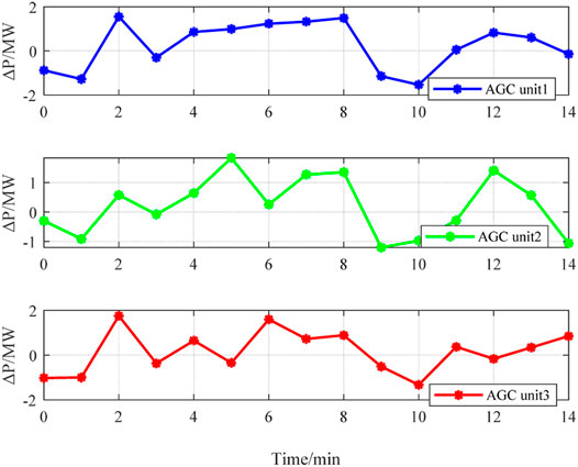
FIGURE 9. Results of AGC regulation curves.
In the training process, the cumulative reward of each episode is recorded. Then, the results and the filtered curve are shown in Figure 10.
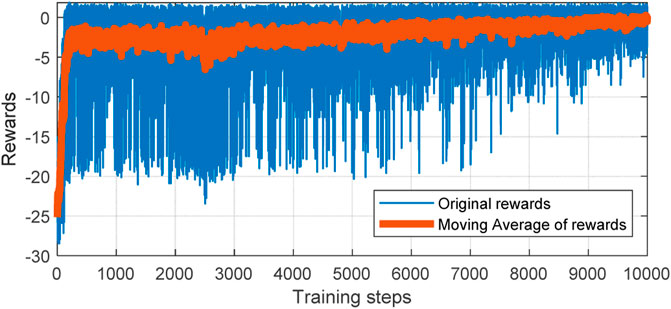
FIGURE 10. Performance of the PPO agent in the training process using 10,000 episodes.
Due to the loads and wind power fluctuations being different in each episode, the needs of frequency regulation in each episode are also different. Therefore, it is normal that there exists slight oscillation of cumulative rewards for each episode. As the training process continues, the cumulative rewards tend to converge as shown in Fig.
To effectively mitigate frequency control issues under growing uncertainties, this article presents a novel solution, the PPO architecture for AGC dynamic optimization, which transformed the traditional optimization problem into a Markov decision process and utilized deep reinforcement learning algorithm for frequency control.
Through the design of state, action, and reward functions, the continuous multiple time step control can be implemented with the goal of maximizing cumulative rewards. The model utilized the way of interaction between the agent and the environment to improve the parameters, which is adaptive to the uncertainties in the environment and avoids the modeling of uncertain variables. The model proposed in this article is tested on the modified IEEE 39 bus system. The results demonstrate that the PPO architecture for AGC dynamic optimization can achieve the goal of frequency control with satisfactory performance compared to other methods. It is verified that the method proposed in this article can effectively solve the stochastic disturbance problem caused by large-scale integration of renewable energy into power grid and ensure the safety and stability of system frequency.
From the lessons learned in this work, the directions of future works are discussed here. First, the deep learning-based algorithms suffered from poor interpretability, which is undesired for control engineering problems. With the developments of explainable artificial intelligence, future works are needed on this direction. Second, better exploration mechanisms for DRL algorithms need to be developed to further improving the training efficiency and avoiding the local optimal solutions.
The raw data supporting the conclusion of this article will be made available by the authors, without undue reservation.
ZL and JL wrote the manuscript. The simulations were performed by JL and PZ. ZD and YZ provided major and minor revisions to the final version of the submitted manuscript. All of the aforementioned authors contributed to the proposed methodology.
This work is supported by the Fundamental Research Funds for the Central Universities under Grant No. 2021JBM027 and the National Natural Science Foundation of China under Grant No. 52107068. Both funds are supportive to open access publication fees.
The authors declare that the research was conducted in the absence of any commercial or financial relationships that could be construed as a potential conflict of interest.
All claims expressed in this article are solely those of the authors and do not necessarily represent those of their affiliated organizations, or those of the publisher, the editors, and the reviewers. Any product that may be evaluated in this article, or claim that may be made by its manufacturer, is not guaranteed or endorsed by the publisher.
1https://www.iso-ne.com/isoexpress/web/reports.
Abdel-Magid, Y. L., and Dawoud, M. M. (1996). Optimal AGC Tuning with Genetic Algorithms. Electr. Power Syst. Res. 38 (3), 231–238. doi:10.1016/s0378-7796(96)01091-7
Atic, N., Rerkpreedapong, D., Hasanovic, A., and Feliachi, A. (2003). “NERC Compliant Decentralized Load Frequency Control Design Using Model Predictive Control[C],” in Power Engineering Society General Meeting (Piscataway, NJ, USA: IEEE).
Banakar, H., Luo, C., and Ooi, B. T. (2008). Impacts of Wind Power Minute-To-Minute Variations on Power System Operation. IEEE Trans. Power Syst. 23 (1), 150–160. doi:10.1109/tpwrs.2007.913298
Beaufays, F., Widrow, B., Abdel-Magid, Y., and Widrow, B. (1994). Application of Neural Networks to Load-Frequency Control in Power Systems. Neural Netw. 7 (1), 183–194. doi:10.1016/0893-6080(94)90067-1
Bohn, E., and Miniesy, S. (1972). Optimum Load-Frequency Sampled-Data Control with Randomly Varying System Disturbances. IEEE Trans. Power Apparatus Syst. PAS-91 (5), 1916–1923. doi:10.1109/tpas.1972.293519
Chang, C. S., Fu, W., and Wen, F. (1998). Load Frequency Control Using Genetic-Algorithm Based Fuzzy Gain Scheduling of Pi Controllers. Electr. Mach. Power Syst. 26 (1), 39–52. doi:10.1080/07313569808955806
Concordia, C., and Kirchmayer, L. K. (1953). Tie-Line Power and Frequency Control of Electric Power Systems. Power Apparatus Syst. Part III Trans. Am. Inst. Electr. Eng. 72 (2), 562–572. doi:10.1109/aieepas.1953.4498667
Dahiya, P., Sharma, V., and Naresh, R. (2016). Automatic Generation Control Using Disrupted Oppositional Based Gravitational Search Algorithm Optimised Sliding Mode Controller under Deregulated Environment. IET Gener. Transm. & Distrib. 10 (16), 3995–4005. doi:10.1049/iet-gtd.2016.0175
Duan, J., Shi, D., Diao, R., Li, H., Wang, Z., Zhang, B., et al. (2020). Deep-Reinforcement-Learning-Based Autonomous Voltage Control for Power Grid Operations. IEEE Trans. Power Syst. 35 (1), 814–817. doi:10.1109/TPWRS.2019.2941134
Elgerd, O. I., and Fosha, C. E. (2007). Optimum Megawatt-Frequency Control of Multiarea Electric Energy Systems[J]. IEEE Trans. Power Apparatus Syst. PAS-89 (4), 556–563.
Erschler, J., Roubellat, F., and Vernhes, J. P. (1974). Automation of a Hydroelectric Power Station Using Variable-Structure Control Systems. Automatica 10 (1), 31–36. doi:10.1016/0005-1098(74)90007-7
Feliachi, A., and Rerkpreedapong, D. (2005). NERC Compliant Load Frequency Control Design Using Fuzzy Rules. Electr. Power Syst. Res. 73 (2), 101–106. doi:10.1016/j.epsr.2004.06.010
Jaleeli, N., VanSlyck, L. S., Ewart, D. N., Fink, L. H., and Hoffmann, A. G. (2002). Understanding Automatic Generation Control[J]. IEEE Trans. Power Syst. 7 (3), 1106–1122. doi:10.1109/59.207324
Jaleeli, N., and Vanslyck, L. S. (1999). NERC's New Control Performance Standards. IEEE Trans. Power Syst. 14 (3), 1092–1099. doi:10.1109/59.780932
Khodabakhshian, A., and Edrisi, M. (2004). A New Robust PID Load Frequency Controller. Control Eng. Pract. 19 (3), 1528–1537. doi:10.1016/j.conengprac.2007.12.003
Mcnamara, P., and Milano, F. (2017). Model Predictive Control Based AGC for Multi-Terminal HVDC-Connected AC Grids[J]. IEEE Trans. Power Syst. 2017, 1.
Olmos, L., de la Fuente, J. I., Zamora Macho, J. L., Pecharroman, R. R., Calmarza, A. M., and Moreno, J. (2004). New Design for the Spanish AGC Scheme Using an Adaptive Gain Controller. IEEE Trans. Power Syst. 19 (3), 1528–1537. doi:10.1109/tpwrs.2004.825873
Pan, I., and Das, S. (2016). Fractional Order AGC for Distributed Energy Resources Using Robust Optimization. IEEE Trans. Smart Grid 7 (5), 2175–2186. doi:10.1109/TSG.2015.2459766
Sahu, B. K., Pati, S., Mohanty, P. K., and Panda, S. (2015). Teaching-learning Based Optimization Algorithm Based Fuzzy-PID Controller for Automatic Generation Control of Multi-Area Power System. Appl. Soft Comput. 27, 240–249. doi:10.1016/j.asoc.2014.11.027
Schulman, J., Wolski, F., Dhariwal, P., Radford, A., and Klimov, O. (2017). Proximal Policy Optimization Algorithms[J]. arXiv:1707.06347.
Schulman, J., Moritz, P., Levine, S., Jordan, M., and Abbeel, P. (2015). High-dimensional Continuous Control Using Generalized Advantage Estimation. arXiv Prepr. arXiv:1506.02438.
Sun, L. (2017). “Analysis and Comparison of Variable Structure Fuzzy Neural Network Control and the PID Algorithm,” in 2017 Chinese Automation Congress (CAC), Jinan, 3347–3350. doi:10.1109/CAC.2017.8243356
Sutton, R. S., and Barto, A. G. (1998). Reinforcement Learning: An Introduction. Cambridge, MA, USA: MIT Press, 3–23.
Talaq, J., and Al-Basri, F. (1999). Adaptive Fuzzy Gain Scheduling for Load Frequency Control. IEEE Trans. Power Syst. 14 (1), 145–150. doi:10.1109/59.744505
Venayagamoorthy, G. K., Sharma, R. K., Gautam, P. K., and Ahmadi, A. (2016). Dynamic Energy Management System for a Smart Microgrid. IEEE Trans. Neural Netw. Learn. Syst. 27 (8), 1643–1656. doi:10.1109/TNNLS.2016.2514358
Wang, B., Li, Y., Ming, W., and Wang, S. (2020). Deep Reinforcement Learning Method for Demand Response Management of Interruptible Load. IEEE Trans. Smart Grid 11 (4), 3146–3155. doi:10.1109/TSG.2020.2967430
Wen, Z., O'Neill, D., and Maei, H. (2015). Optimal Demand Response Using Device-Based Reinforcement Learning. IEEE Trans. Smart Grid 6 (5), 2312–2324. doi:10.1109/TSG.2015.2396993
Xi, L., Zhou, L., Xu, Y., and Chen, X. (2021). A Multi-step Unified Reinforcement Learning Method for Automatic Generation Control in Multi-Area Interconnected Power Grid. IEEE Trans. Sustain. Energy 12 (2), 1406–1415. doi:10.1109/TSTE.2020.3047137
Yamashita, K., and Taniguchi, T. (1986). Optimal Observer Design for Load-Frequency Control. Int. J. Electr. Power & Energy Syst. 8 (2), 93–100. doi:10.1016/0142-0615(86)90003-7
Yan, W., Zhao, R., Zhao, X., Li, Y., Yu, J., and Li, Z. (2012). Dynamic Optimization Model of AGC Strategy under CPS for Interconnected Power System[J]. Int. Rev. Electr. Eng. 7 (5PT.B), 5733–5743.
Yu, T., Zhou, B., Chan, K. W., Chen, L., and Yang, B. (2011). Stochastic Optimal Relaxed Automatic Generation Control in Non-markov Environment Based on Multi-step Q(λ) Learning. IEEE Trans. Power Syst. 26 (3), 1272–1282. doi:10.1109/TPWRS.2010.2102372
Zeynelgil, H. L., Demiroren, A., and Sengor, N. S. (2002). The Application of ANN Technique to Automatic Generation Control for Multi-Area Power System. Int. J. Electr. Power & Energy Syst. 24 (5), 345–354. doi:10.1016/s0142-0615(01)00049-7
Zhang, X. S., Li, Q., Yu, T., and Yang, B. (2016). Consensus Transfer Q-Learning for Decentralized Generation Command Dispatch Based on Virtual Generation Tribe. IEEE Trans. Smart Grid 9 (3), 1. doi:10.1109/TSG.2016.2607801
Zhang, X. S., Yu, T., Pan, Z. N., Yang, B., and Bao, T. (2018). Lifelong Learning for Complementary Generation Control of Interconnected Power Grids with High-Penetration Renewables and EVs. IEEE Trans. Power Syst. 33 (4), 4097–4110. doi:10.1109/TPWRS.2017.2767318
Zhang, X., Tan, T., Zhou, B., Yu, T., Yang, B., and Huang, X. (2021). Adaptive Distributed Auction-Based Algorithm for Optimal Mileage Based AGC Dispatch with High Participation of Renewable Energy. Int. J. Electr. Power & Energy Syst. 124, 106371. doi:10.1016/j.ijepes.2020.106371
Zhang, X., Xu, Z., Yu, T., Yang, B., and Wang, H. (2020). Optimal Mileage Based AGC Dispatch of a GenCo. IEEE Trans. Power Syst. 35 (4), 2516–2526. doi:10.1109/TPWRS.2020.2966509
Zhang, X., Yu, T., Yang, B., and Jiang, L. (2021). A Random Forest-Assisted Fast Distributed Auction-Based Algorithm for Hierarchical Coordinated Power Control in a Large-Scale PV Power Plant. IEEE Trans. Sustain. Energy 12 (4), 2471–2481. doi:10.1109/TSTE.2021.3101520
Zhang, X., Yu, T., Yang, B., and Li, L. (2016). Virtual Generation Tribe Based Robust Collaborative Consensus Algorithm for Dynamic Generation Command Dispatch Optimization of Smart Grid. Energy 101, 34–51. doi:10.1016/j.energy.2016.02.009
Zhao, X., Ye, X., Yang, L., Zhang, R., and Yan, W. (2018). Chance Constrained Dynamic Optimisation Method for AGC Units Dispatch Considering Uncertainties of the Offshore Wind Farm[J]. J. Eng. 2019 (16), 2112. doi:10.1049/joe.2018.8558
Keywords: automatic generation control, advanced optimization strategy, deep reinforcement learning, renewable energy, proximal policy optimization
Citation: Liu Z, Li J, Zhang P, Ding Z and Zhao Y (2022) An AGC Dynamic Optimization Method Based on Proximal Policy Optimization. Front. Energy Res. 10:947532. doi: 10.3389/fenrg.2022.947532
Received: 18 May 2022; Accepted: 07 June 2022;
Published: 13 July 2022.
Edited by:
Bo Yang, Kunming University of Science and Technology, ChinaReviewed by:
Xiaoshun Zhang, Northeastern University, ChinaCopyright © 2022 Liu, Li, Zhang, Ding and Zhao. This is an open-access article distributed under the terms of the Creative Commons Attribution License (CC BY). The use, distribution or reproduction in other forums is permitted, provided the original author(s) and the copyright owner(s) are credited and that the original publication in this journal is cited, in accordance with accepted academic practice. No use, distribution or reproduction is permitted which does not comply with these terms.
*Correspondence: Zhao Liu, bGl1emhhbzFAYmp0dS5lZHUuY24=; Pei Zhang, MjUxMjY5MjU3N0BxcS5jb20mI3gwMjAwYTs=
Disclaimer: All claims expressed in this article are solely those of the authors and do not necessarily represent those of their affiliated organizations, or those of the publisher, the editors and the reviewers. Any product that may be evaluated in this article or claim that may be made by its manufacturer is not guaranteed or endorsed by the publisher.
Research integrity at Frontiers
Learn more about the work of our research integrity team to safeguard the quality of each article we publish.