Numerical Study of Low Pr Flow in a Bare 19-Rod Bundle Based on an Advanced Turbulent Heat Transfer Model

Compared to assuming a constant turbulent Prandtl number model, an advanced four-equation model has the potential to improve the numerical heat transfer calculation accuracy of low–Prandtl number $\left(Pr\right)$ fluids. Generally, a four-equation model consists of a two-equation $k-\epsilon$ turbulence model and a two-equation $k_{\theta }-{\epsilon }_{\theta }$ heat transfer model. It is essential to analyze the influence of dissimilar turbulence models on the overall calculation accuracy of the four-equation model. The present study aims to study the effect of using different turbulence models on the same $k_{\theta }-{\epsilon }_{\theta }$ heat transfer model. First, based on the open-source computational fluid dynamics software OpenFOAM, an advanced two-equation $k_{\theta }-{\epsilon }_{\theta }$ heat transfer model was introduced into the solver buoyant2eqnFoam, which was developed based on the self-solver buoyantSimpleFoam of OpenFOAM. In the solver buoyant2eqnFoam, various turbulence models built into OpenFOAM can be conveniently called to close the Reynolds stress and an advanced two-equation heat transfer model can be utilized to calculate the Reynolds heat flux of low-$Pr$ fluids. Subsequently, the solver buoyant2eqnFoam was employed to study the fully developed flow heat transfer of low-$Pr$ fluids in a bare 19-rod bundle. The numerical results were compared and analyzed with the experimental correlations and other simulation results to validate the effectiveness and feasibility of the solver buoyant2eqnFoam. Furthermore, the influence of combining different turbulence models with the same two-equation $k_{\theta }-{\epsilon }_{\theta }$ heat transfer model was also presented in this study. The results show that the turbulence model has a considerable influence on the prediction of turbulent heat transfer in the high Peclet number range, suggesting that it should be prudent when picking a turbulence model in the simulations of low-$Pr$ fluids.

1 Introduction

Nuclear energy is playing an increasingly irreplaceable role in the future energy structure as the demand for energy increases rapidly (Gu and Su, 2021). Lead-cooled fast reactor (LFR) is one of the six types of innovative nuclear power systems proposed by the Generation IV International Forum (Abram and Ion, 2008; Pacio et al., 2015). Benefiting from the excellent performance in chemical inertness, neutron economy, and thermohydraulic properties, lead–bismuth eutectic (LBE) is considered as one of most promising coolants for LFR. It is indispensable to research the thermohydraulic behaviors of the LBE inner fuel assembly, which influences the security and economic performance of LFRs but is poorly understood (Martelli et al., 2017; Pacio et al., 2017).

Since it is expensive, parlous, and complicated to conduct an experiment with LBE under a high-temperature state, computational fluid dynamics (CFD) methods are widely employed to study the thermohydraulic characteristics of LBE. The CFD methods can be subdivided into three categories: direct numerical simulation (DNS), large eddy simulation (LES), and Reynolds-averaged Navier–Stokes simulation (RANS). Despite the high calculation accuracy of DNS and LES, they have a high demand for computational resources, and as a result, they are only suitable for some specific and straightforward geometric models (Kawamura et al., 1999). Since the computational cost of the RANS approach is much lower than that of the DNS and LES, the RANS approach is the most widely adopted CFD method in engineering calculation. In the RANS method, the linear eddy-viscosity $k-\epsilon$ or $k-\omega$ turbulence model is ordinarily sufficient to accurately predict the momentum transport of various fluids (Nagano, 2002). On the other hand, for reproducing the heat transfer, the Reynolds-analogy hypothesis assuming a constant turbulent Prandtl number $P{r}_t=0.85\sim 0.9$ is adopted in almost all commercial codes (Manservisi and Menghini, 2014a). For the simulation of ordinary fluids like water and air, having a relatively high Prandtl number, the rational results can be obtained with a constant $P{r}_t$ (He et al., 2021). However, LBE is characterized by high thermal diffusivity and low viscosity values, resulting in low Prandtl numbers ($Pr\approx 0.01\sim 0.03$). Consequently, the Reynolds-analogy hypothesis is no longer appropriate to be employed to study the thermohydraulic characteristics of LBE by the CFD methods (Cheng and Tak, 2006). For this reason, some advanced turbulent heat transfer models which can reproduce the heat transfer behaviors of LBE with high precision are highly desirable.

In the past four decades, to improve the calculation accuracy of heat transfer for low-$Pr$ fluids, various heat flux models to close the energy conservation equation in the framework of RANS have been developed.

1.1 Differential Heat Flux Model

DHFM is a full second-moment differential model for the transport of Reynolds heat fluxes. Compared with the constant $P{r}_t$ model, DHFM fully considers the convection, diffusion, generation, and dissipation terms of Reynolds heat flux in the differential equations. Carteciano (1995), Carteciano et al. (1997), Carteciano et al. (2001), and Carteciano and Grötzbach (2003) developed a kind of DHFM named turbulence model for buoyant flows (TMBF). The simulations of two-dimensional forced convection and mixed convection with different fluids were carried out to evaluate the accuracy of TMBF. The numerical results obtained by TMBF demonstrate that stratified flows and buoyant effects were well reproduced compared with the constant $P{r}_t$ model, especially in mixed convection conditions. Based on a summary of the various DHFM models developed in recent years, Shin et al. (2008) proposed a new set of DHFM models with an elliptic blending model. The new model was utilized to study the fully developed square duct flow, rotating, and nonrotating channel flow. The numerical results show good agreement with the LES and DNS results.

1.2 Algebraic Heat Flux Model

AHFM is a simplified second-moment form of DHFM, which transports Reynolds heat flux by establishing algebraic equations. Hanjalić et al. (1996), Kenjereš et al. (2005), Otić et al. (2005), and Otić and Grotzbach. (2007) developed and analyzed an implicit algebraic transport equation for the Reynolds heat flux term to close the energy equation. Evaluations and calibrations of AHFM for low-$Pr$ fluids were implemented by Shams et al. (2014), Shams (2018), Shams et al. (2018), and De Santis et al. (2018) and De Santis and Shams (2018). AHFM has been validated in their works by comparison with the DNS data for turbulent flows in forced, mixed, and natural convection of different fluids. The numerical results obtained by AHFM illustrate that temperature, heat flux field, buoyant effects in-plane, backward-facing step, corium pool, rod bundle, etc. are well predicted.

1.3 A two-equation $k_{\theta }-{\epsilon }_{\theta }$ model for Reynolds heat flux

The $k_{\theta }-{\epsilon }_{\theta }$ model is a first-order 2-equation model for the calculation of Reynolds heat flux, which can be developed in a way similar to that of a first-order 2-equation $k-\epsilon$ model for the turbulent transport of momentum formulated. Compared with DHFM and AHFM, the two-equation model has been widely applied in recent years because of its lower calculation cost. To precisely reproduce the heat transfer of low-$Pr$ fluids, extensive contributions of model coefficient and function, wall boundary conditions, and near-wall thermal turbulence effect of a two-equation $k_{\theta }-{\epsilon }_{\theta }$ model had been made by Nagano and Kim (1988); Nagano and Shimada (1996); Nagano et al. (1997); Nagano (2002), Sommer et al. (1992), and Youssef et al. (1992); and Youssef (2006), Abe et al. (1994), Hattori et al. (1993), Hwang and Lin (1999), Deng et al. (2001), and Karcz and Badur (2005). In recent years, based on previous study, Manservisi and Menghini (2014a); Manservisi and Menghini (2014b); Manservisi and Menghini (2015), Cerroni et al. (2015), Cervone et al. (2020), Chierici et al. (2019), and Da Via et al. (2016); Da Vià and Manservisi (2019); and Da Vià et al. (2020) proposed a two-equation $k_{\theta }-{\epsilon }_{\theta }$ model suitable for the LBE turbulent heat transfer simulation, and improved new numerical near-wall boundary conditions for turbulence variables. The numerical results obtained by the literature (Manservisi and Menghini, 2014a; Manservisi and Menghini, 2014b; Manservisi and Menghini, 2015; Su et al., 2022) indicate that turbulent heat transfer statistics such as in-plane, tube, backward-facing step, triangular rod bundle, square lattice bare rod bundle, and hexagonal rod bundle of forced convection of LBE are well reproduced based on their $k_{\theta }-{\epsilon }_{\theta }$ turbulent heat transfer model.

In recent years, the interest in reliable CFD methods used to investigate the turbulent heat transfer of low-$Pr$ fluids in complicated industrial configurations has increased dramatically. Nevertheless, commercial codes are still lacking, except for an AHFM model available on software STAR-CCM+ (Simcenter, 2016). A two-equation $k-\epsilon$ model utilized to calculate Reynolds stress with a two-equation $k_{\theta }-{\epsilon }_{\theta }$ model used to calculate Reynolds heat flux is usually called a four-equation $k-\epsilon -k_{\theta }-{\epsilon }_{\theta }$ model, which is expected to improve the numerical CFD accuracy of turbulent heat transfer for LBE. However, different turbulence models will have a certain impact on the time-scale transport of a two-equation $k_{\theta }-{\epsilon }_{\theta }$ model. It is necessary to evaluate the sensitivity of various turbulence models to a two-equation $k_{\theta }-{\epsilon }_{\theta }$ model.

Thus, in the present study, an improved CFD solver buoyant2eqnFoam, which introduces a two-equation $k_{\theta }-{\epsilon }_{\theta }$ model to calculate the Reynolds heat flux and can directly call different turbulence models to calculate the Reynolds stress, was first developed based on the solver buoyantSimpleFoam of open-source CFD program OpenFOAM. The fully developed turbulent heat transfer results of LBE inner flow and a bare 19-rod bundle geometry with different Peclet numbers were investigated and compared with experimental relations to verify the effectiveness of the solver buoyant2eqnFoam and the numerical algorithm. Finally, the heat transfer sensitivity of different turbulence models to the two-equation $k_{\theta }-{\epsilon }_{\theta }$ model was presented.

2 Mathematical Model

2.1 Physical Model

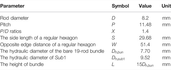
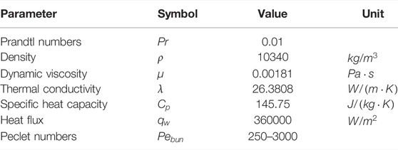
Thermal-hydraulic phenomena in a 19-rod bundle geometry are an essential research topic. In the past decades, numerous experimental and simulation researches have been conducted to precisely obtain flow characteristics and heat transfer correlations of coolant (Pacio et al., 2014; Martelli et al., 2017). In the present study, a bare 19-rod bundle with a fully developed turbulent LBE flow is considered. Figure 1A displays the cross section of the bare 19-rod bundle. Since the cross-flow in the bare 19-rod bundle is negligible and its construction is symmetrical, one-twelfth of the whole bundle is selected to carry out simulation for the sake of economizing computational cost. The computational domain is sketched in Figure 1B, together with the definitions of sub-channels and boundary regions. $Sub1$, $Sub2$, and $Sub3$ are defined as inner sub-channels, while $Sub4$ and $Sub5$ are the edge sub-channel and corner sub-channel, respectively. The more detailed geometric parameters are summarized in Table 1, which are consistent with Pacio’s experiment (Pacio et al., 2015), except that there are no grid spacers in the current study. $D_{h,bun}$ and $D_{h,sub1}$ are the hydraulic diameter of the bundle and hydraulic diameter of $Sub1$, respectively. The length of the whole computational domain is set to 15 $D_{h,bun}$ to eliminate the effect of employing periodic inlet boundary conditions. The flow parameters of LBE are reported in Table 2, where $P{e}_{bun}=Pr{U}_{bun}{D}_{h,bun}\rho /\mu$ is the Peclet number of the bundle.

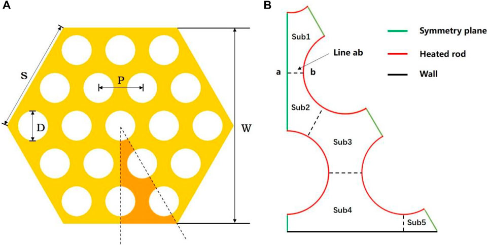
FIGURE 1

FIGURE 1. Diagrammatic sketch of the bare 19-rod bundle. (A) Cross section and (B) computational domain.

TABLE 1

TABLE 1. Geometric parameters of the bare 19-rod bundle.

TABLE 2

TABLE 2. Flow parameters of LBE.

2.2 Conservation Equations

For forced convection, the incompressible RANS equations with constant physical properties and no gravity are considered

$\frac{\partial u_i}{\partial x_i}=0(1)$

$\frac{\partial u_i}{\partial t}+u_j\frac{\partial u_i}{\partial x_j}=-\frac{1}{\rho }\frac{\partial P}{\partial x_i}+\frac{\partial }{\partial x_j}\left(v\frac{\partial u_i}{\partial x_j}\right)-\frac{\partial }{\partial x_j}\overline{u_i^{\prime }{u}_j^{\prime }}(2)$

where $\nu$, $u_i$, and $P$ are the molecular viscosity, Reynolds-averaged velocity, and the so-called average pressure, respectively. To obtain the unknown Reynolds stress $\overline{{u^{\prime }}_i{u^{\prime }}_j}$, the linear eddy-viscosity model can be adopted as follows:

$\overline{{u^{\prime }}_i{u^{\prime }}_j}=-v_t\left(\frac{\partial u_i}{\partial x_j}+\frac{\partial u_j}{\partial x_i}\right)+\frac{2k}{3}{\delta }_{ij}(3)$

where $k$ and ${\nu }_t$, both derived from the turbulence model, represent the turbulent kinetic energy and the turbulent viscosity, respectively.

It should be noted that, in OpenFOAM, the energy conservation equation can be expressed in terms of enthalpy (Darwish and Moukalled, 2021):

$\frac{\partial h}{\partial t}+u_j\frac{\partial h}{\partial x_j}+\frac{\partial K}{\partial t}+u_j\frac{\partial K}{\partial x_j}=\frac{1}{\rho }\frac{\partial P}{\partial t}+\frac{\partial }{\partial x_j}\left(\left(\alpha +{\alpha }_t\right)\frac{\partial h}{\partial x_j}\right)(4)$

where $h$, $K={\left|U\right|}^2/2$, $\alpha$, and ${\alpha }_t$ are the enthalpy per unit of mass, the kinetic energy per unit of mass, molecular thermal diffusivity, and the turbulent thermal diffusivity, respectively. The unknown ${\alpha }_t$ needs to be derived from a two-equation $k_{\theta }-{\epsilon }_{\theta }$ turbulent heat transfer model. After solving Eq. 4, the distribution of $h$ can be obtained. Subsequently, the Reynolds-averaged temperature $T$ can be calculated by using the function Thermo.T () coming with OpenFOAM. The derivation of periodic momentum and energy equations in OpenFOAM can be found in the reference (Ge et al., 2017).

2.3 Turbulence Model for Momentum Field

Benefiting from replacing the friction velocity $u_{\tau }$ with Kolmogorov velocity $u_{\epsilon }$, the turbulence model proposed by Abe et al. (1994), which can well reproduce the low Reynolds number and near-wall effects of both separated and attached flows, was widely adopted in the calculation of LBE (Manservisi and Menghini, 2014a; Manservisi and Menghini, 2014b; Cerroni et al., 2015; Manservisi and Menghini, 2015; Da Via et al., 2016; Chierici et al., 2019; Da Vià and Manservisi, 2019; Cervone et al., 2020; Da Vià et al., 2020). However, the Abe $k-\epsilon$ turbulence model does not exist in the current turbulence model library of OpenFOAM. Therefore, in the current study, the Abe $k-\epsilon$ turbulence model is compiled into the turbulence model library that comes with OpenFOAM so as to utilize the wall functions of OpenFOAM in this self-compiled turbulence model. In the Abe $k-\epsilon$ turbulence model, the turbulent viscosity ${\nu }_t$ is computed as follows:

$v_{\text{t}}=C_{\mu }{f}_{\mu }\frac{k^2}{\epsilon }(5)$

where $C_{\mu }$ is a constant. $f_{\mu }$ is the model function, defined as follows:

$f_{\mu }={\left(1-\exp \left(-\frac{y^{\ast }}{14}\right)\right)}^2\left(1+\frac{5}{R_t^{3/4}}\exp \left(-{\left(\frac{R_t}{200}\right)}^2\right)\right)(6)$

$y^{\ast }=\frac{u_{\epsilon }\delta }{\nu }(7)$

where $R_t=k^2/\nu \epsilon$ and $u_{\epsilon }={\left(\nu \epsilon \right)}^{1/4}$. Moreover, $\delta$ is the distance from the wall. The equations for $k$ and its dissipation $\epsilon$ can be written as follows:

$\frac{\partial k}{\partial t}+u_j\frac{\partial k}{\partial x_j}=\frac{\partial }{\partial x_j}\left(\left(v+\frac{v_t}{{\sigma }_k}\right)\frac{\partial k}{\partial x_j}\right)+P_k-\epsilon (8)$

$P_k=-\overline{u_i^{\prime }{u}_j^{\prime }}\frac{\partial u_i}{\partial x_j}=v_t\left(\frac{\partial u_i}{\partial x_j}+\frac{\partial u_j}{\partial x_i}\right)\frac{\partial u_i}{\partial x_j}-\frac{2k{\delta }_{ij}}{3}\frac{\partial u_i}{\partial x_j}(9)$

$\frac{\partial \epsilon }{\partial t}+u_j\frac{\partial \epsilon }{\partial x_j}=\frac{\partial }{\partial x_j}\left(\left(v+\frac{v_t}{{\sigma }_{\epsilon }}\right)\frac{\partial \epsilon }{\partial x_j}\right)+C_{1\epsilon }\frac{\epsilon }{k}{P}_k-C_{2\epsilon }{f}_{\epsilon }\frac{{\epsilon }^2}{k}(10)$

$f_{\epsilon }={\left(1-\exp \left(-\frac{y^{\ast }}{3.1}\right)\right)}^2\left(1-0.3\exp \left(-\frac{R_t^2}{6.5}\right)\right)(11)$

The model constants utilized in the Abe $k-\epsilon$ turbulence model are reported in Table 3.

TABLE 3

TABLE 3. The model constants of the Abe $k-\epsilon$ turbulence model.

2.4 Two-Equation Model for Thermal Field

In the current work, the $k_{\theta }-{\epsilon }_{\theta }$ turbulent heat transfer model developed and improved by Manservisi and Menghini (2014a), Manservisi and Menghini (2014b), and Manservisi and Menghini (2015), which introduces the average square temperature fluctuation $k_{\theta }$ and its dissipation ${\epsilon }_{\theta }$ in order to well reproduce the near-wall turbulent heat transfer behaviors of LBE having $Pr$ in the range of 0.01–0.03, is adopted to calculate the turbulent thermal diffusivity ${\alpha }_t$. In the Manservisi $k_{\theta }-{\epsilon }_{\theta }$ model, ${\alpha }_t$ is computed as follows:

${\alpha }_t=C_{\theta }k{\tau }_{l\theta }(12)$

where $C_{\theta }$ is the constant empirical coefficient and ${\tau }_{l\theta }$ is the local thermal characteristic time, modeled as follows:

${\tau }_{l\theta }=f_{1\theta }{B}_{1\theta }+f_{2\theta }{B}_{2\theta }(13)$

with the appropriate functions set as follows:

$f_{1\theta }=\left(1-\exp \left(-\frac{R_{\delta }}{19\sqrt{Pr}}\right)\right)\left(1-\exp \left(-\frac{R_{\delta }}{14}\right)\right)(14)$

$B_{1\theta }=0.9{\tau }_{\text{u}}=0.9\frac{k}{\epsilon }(15)$

$f_{2\theta }{B}_{2\theta }={\tau }_u\left(f_{2a\theta }\frac{2R}{R+C_{\gamma }}+f_{2b\theta }\sqrt{\frac{2R}{Pr}}\frac{1.3}{\sqrt{Pr}{R}_t^{3/4}}\right)(16)$

$f_{2a\theta }=f_{1\theta }\exp \left(-{\left(\frac{R_t}{500}\right)}^2\right)(17)$

$f_{2b\theta }=f_{1\theta }\exp \left(-{\left(\frac{R_{\delta }}{200}\right)}^2\right)(18)$

where $R_{\delta }=\delta {\epsilon }^{1/4}/{\nu }^{3/4}$, ${\tau }_u=k/\epsilon$, and $R={\tau }_{\theta }/{\tau }_u$ with the thermal turbulent characteristic time ${\tau }_{\theta }=k_{\theta }/{\epsilon }_{\theta }$. In addition, ${\tau }_u=k/\epsilon$ represents the dynamical turbulent characteristic time. The equations for $k_{\theta }$ and its dissipation ${\epsilon }_{\theta }$ can be written as follows:

$\frac{\partial k_{\theta }}{\partial t}+u_j\frac{\partial k_{\theta }}{\partial x_j}=\frac{\partial }{\partial x_j}\left(\left(\alpha +\frac{{\alpha }_t}{{\sigma }_{k_{\theta }}}\right)\frac{\partial k_{\theta }}{\partial x_j}\right)+P_{\theta }-{\epsilon }_{\theta }(19)$

$P_{\theta }={\alpha }_t\left(\frac{\partial T}{\partial x_j}\right)\left(\frac{\partial T}{\partial x_j}\right)(20)$

$\begin{array}{l}\frac{\partial {\epsilon }_{\theta }}{\partial t}+u_j\frac{\partial {\epsilon }_{\theta }}{\partial x_j}=\frac{\partial }{\partial x_j}\left(\left(\alpha +\frac{{\alpha }_t}{{\sigma }_{{\epsilon }_{\theta }}}\right)\frac{\partial {\epsilon }_{\theta }}{\partial x_j}\right)+\frac{{\epsilon }_{\theta }}{k_{\theta }}\left(C_{P1}{P}_{\theta }-C_{d1}{\epsilon }_{\theta }\right)\\ +\frac{{\epsilon }_{\theta }}{k}\left(C_{P2}{P}_k-C_{d2}\epsilon \right)\end{array}(21)$

$C_{d2}=\left(1.9\left(1-0.3\exp \left(-{\left(\frac{R_t}{6.5}\right)}^2\right)\right)-1\right){\left(1-\exp \left(-\frac{R_{\delta }}{5.7}\right)\right)}^2(22)$

The constant empirical coefficients used in the Manservisi $k_{\theta }-{\epsilon }_{\theta }$ turbulent heat transfer are reported in Table 4.

TABLE 4

TABLE 4. The constant empirical coefficients of the Manservisi $k_{\theta }-{\epsilon }_{\theta }$ turbulent heat transfer model.

3 Solver and Boundary Conditions

To calculate the thermal-hydraulic characteristics of LBE, a CFD solver named buoyant2eqnFoam was developed on the OpenFOAM platform having user-friendly programming language features based on the turbulence model and the aforementioned turbulent heat transfer model. The SIMPLE algorithm is adopted to handle pressure–velocity coupling equations and the coupled multigrid iterations technique is utilized for matrix solutions. All calculations were performed using double precision on OpenFOAM and the convergence conditions of residual error are set as follows:

$\text{Max}\left|\frac{Q^{n+1}}{Q^n}-1\right|<{10}^{-6}(23)$

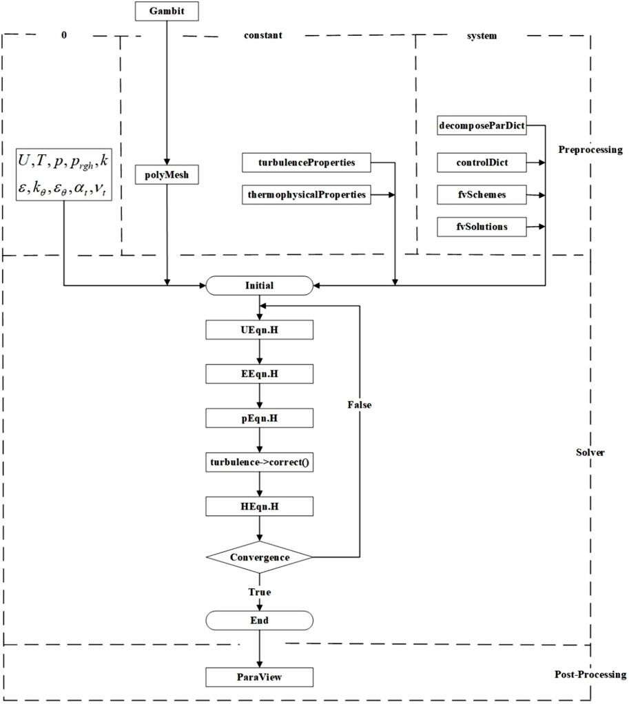
where $Q$ stands for $u_i,T,P,k_{\theta },{\epsilon }_{\theta },k$, and $\epsilon$. The index $i$ represents the number of iterations. The framework of the buoyant2eqnFoam solver is presented in Figure 2. The buoyant2eqnFoam solver mainly includes main-program buoyant2eqnFoam.C, velocity equation UEqn.H, energy equation EEqn.H, pressure–Poisson equation pEqn.H, call function of turbulence model turbulence- > correct(), and a two-equation $k_{\theta }-{\epsilon }_{\theta }$ heat transfer model HEqn.H. The boundary condition data, mesh data, physical property data, calculation control, discrete format of each differential operator, algebraic equation solver, and relaxation factor required by buoyant2eqnFoam to perform calculation are included in the 0 folder, constant/polyMesh, constant/thermophysicalProperties, system/controlDict, system/fvSchemes, and system/fvSolutions.

FIGURE 2

FIGURE 2. Framework of the buoyant2eqnFoam solver in OpenFOAM.

In the computational domain, periodic boundary conditions are set on the region of inlet and outlet, considering the fully developed turbulent inner flow in the bundle. It is worth noting that the energy source term needs to be added to the energy Eq. 4 in order to apply periodic boundary conditions to temperature variables. The calculation method of energy source term refers to this literature (Ge et al., 2017). For $k_{\theta }$ and ${\epsilon }_{\theta }$, the boundary condition zeroGradient is employed on the wall under the uniform heat flux condition, according to the research of Deng et al. (2001). The boundary conditions imposed on each boundary are summarized in Table 5. Since the wall functions kLowReWallFunction for $k$ and epsilonWallFunction for $\epsilon$ are both suitable for the low–Reynolds number turbulence model and can well reproduce the near-wall turbulence behaviors when $y^{+}$ is very low (Darwish and Moukalled, 2021), they are employed in this study. Given that there are no wall functions accessible for $k_{\theta }$ and ${\epsilon }_{\theta }$ in OpenFOAM, $y^{+}$ must be less than or equal to 1 in order to accurately reproduce the thermal turbulent behaviors near the wall (Manservisi and Menghini, 2014a).

TABLE 5

TABLE 5. Boundary conditions imposed on each boundary.

4 Results and Discussions

4.1 Mesh Independence Analysis

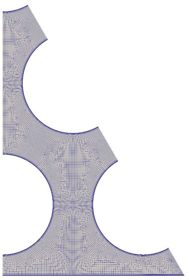
In this section, the buoyant2eqnFoam, which utilizes the Abe $k-\epsilon$ turbulence model for turbulence fields and uses the Manservisi $k_{\theta }-{\epsilon }_{\theta }$ model for thermal fields, is employed to investigate the thermohydraulic characteristics of LBE inner flow in the bare 19-rod bundle in a wide range of $P{e}_{bun}$. As shown in Figure 3, the computational domain was discretized by GAMBIT unstructured meshes (tetrahedral and hexahedral mesh blending). The first layer grid was set with a height of 0.001 mm in order to satisfy the criterion of the low–Reynolds number turbulence model for $y^{+}\le 1$. A total of 15 layers of boundary grids with a height ratio of 1.3 were designed.

FIGURE 3

FIGURE 3. The mesh of computational domain.

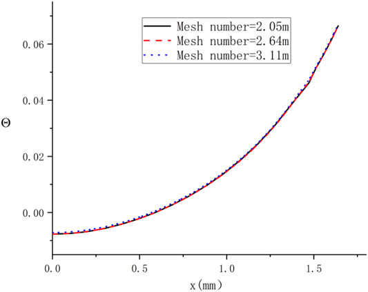
Three sets of mesh with different mesh numbers of 2.05 million, 2.64 million, and 3.11 million were adopted to analyze the mesh sensitivity. The dimensionless coolant temperature $\text{Θ}$ is defined as follows:

$\mathrm{\Theta }=\frac{\left(T-T_{b,bun}\right)\lambda }{D_{h,bun}\cdot q_w}(24)$

where $T_{b,bun}$ is the bulk temperature of the computational domain. The dimensionless temperature profiles along line ab (shown in Figure 1B) of three sets of mesh are displayed in Figure 4 under $P{e}_{bun}=1500$. It is evident that the difference in the dimensionless temperature profile between three sets of mesh is negligible. Consequently, the mesh with a mesh number of 2.05 million is selected, taking the calculation cost into consideration.

FIGURE 4

FIGURE 4. The dimensionless temperature profiles along line ab of the three sets of mesh.

4.2 Solver Verification

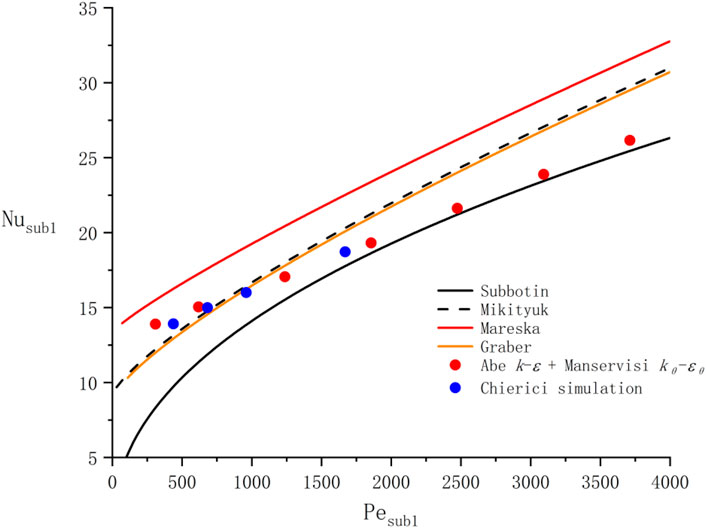
The fully developed turbulent heat transfer characteristics of LBE inner flow in the bare 19-rod bundle were studied by Chierici et al. (2019), using a four-equation model in logarithmic specific dissipation form $k-\text{Ω}-k_{\theta }-{\text{Ω}}_{\theta }$, which was developed based on the Abe $k-\epsilon$ turbulence model and the Manservisi $k_{\theta }-{\epsilon }_{\theta }$ model. The numerical results of Chierici et al. (2019) can provide some reference for developing a CFD solver of LBE turbulent heat transfer. Therefore, the simulation results of Chierici et al. (2019) and some experimental data are picked for comparison to verify the validity of the solver buoyant2eqnFoam. The Nusselt number is selected for comparison since it is a critical parameter in engineering. Table 6 presents some Nusselt number experimental correlations of the triangular rod bundle channel cooled by liquid metal, obtained by Subbotin et al. (1965), Mikityuk (2009), Gräber and Rieger (1972), and Mareska and Dwyer (1964), respectively.

TABLE 6

TABLE 6. Correlations of the Nusselt number for triangular lattices.

Because these reported correlations were developed for triangular lattices, the Nusselt number of inner sub-channel $Sub1$ is picked for comparison. The $N{u}_{sub1}$ is calculated as follows:

$N{u}_{sub1}=\frac{q_w{D}_{h,sub1}}{\lambda \left(T_{w,sub1}-T_{b,sub1}\right)}(25)$

where $T_{w,sub1}$ and $T_{b,sub1}$ are the mean wall temperature and mean coolant temperature of $Sub1$, respectively. Correspondingly, $P{e}_{sub1}=Pr{U}_{sub1}{D}_{h,sub1}\rho /\mu$ is the Peclet number of the inner sub-channel $Sub1$. Figure 5 displays the comparison of the Nusselt number with Chierici simulation and experimental correlations. From this figure, it can be clearly observed that the tendency of $N{u}_{sub1}$ is consistent with the simulation results of Chierici and shows good agreements with experimental data in a specific Peclet number range, illustrating that the rational prediction of LBE turbulent heat transfer can be obtained by the self-compiled solver buoyant2eqnFoam which can use the Abe $k-\epsilon$ turbulence model with wall functions for turbulence fields and the Manservisi $k_{\theta }-{\epsilon }_{\theta }$ model with zero-gradient boundary for thermal fields.

FIGURE 5

FIGURE 5. Comparison of the Nusselt number with Chierici simulation and experimental correlations.

4.3 Flow and Heat Transfer Analysis

4.3.1 Velocity Field

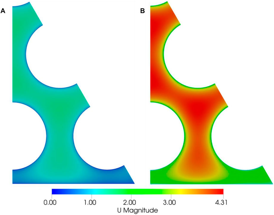
The profiles of velocity magnitude on the computational domain of the bare 19-rod bundle are reported in Figure 6, with $P{e}_{bun}=500$ and $P{e}_{bun}=1500$, respectively. It is obvious that the mean velocity in the inner sub-channels is higher than that in the edge sub-channel $Sub4$ and corner sub-channel $Sub5$ because the hydraulic diameter of inner sub-channels is relatively higher, resulting in much lower flow resistance. For the same reason, the average velocity of $Sub5$ is much lower compared with that of other sub-channels, as summarized in Table 7.

FIGURE 6

FIGURE 6. Profiles of velocity magnitude on a computational domain. (A) $P{e}_{bun}=500$ and (B) $P{e}_{bun}=1500.$

TABLE 7

TABLE 7. Mean velocity of each sub-channel.

4.3.2 Dimensionless Temperature and Hot Spot Factor Distributions

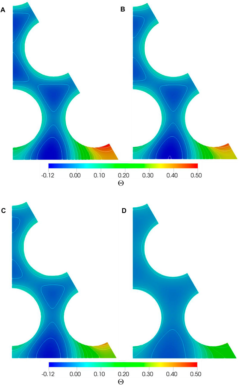
Figure 7 shows the distribution of dimensionless temperature from where it can be seen that the maximum temperature is located in the corner sub-channel $Sub5$, which is mainly due to the lower mean coolant velocity of the corner sub-channel $Sub5$. Owing to the larger hydraulic diameter of the edge sub-channel $Sub4$ and the adiabatic boundary condition applied on the outer casing wall, the coolant with the lowest temperature can be found in the area of the edge sub-channel $Sub4$ near the outer casing wall. Comparing the four cases reported in Figure 7, it can be found that the convective heat transfer of the coolant in each sub-channel is enhanced as the Reynolds number increases, leading to the decrease of maximum temperature and the increase of bulk coolant temperature.

FIGURE 7

FIGURE 7. Profiles of dimensionless temperature on computational domain. (A) $P{e}_{bun}=250$; (B) $P{e}_{bun}=500$; (C) $P{e}_{bun}=1000$; and (D) $P{e}_{bun}=3000.$

The dimensionless hot spot factor characterizing the inhomogeneity of wall temperature is defined as follows:

$\varphi =\frac{{\theta }_{wmax,sub}-{\theta }_{b,sub}}{{\theta }_{wb,sub}-{\theta }_{b,sub}}(26)$

where ${\theta }_{wmax,sub}$, ${\theta }_{b,sub}$, and ${\theta }_{wb,sub}$ are the maximum wall temperature of the sub-channel, the bulk temperature of the sub-channel, and the mean wall temperature of the sub-channel, respectively. As $\varphi =1$, it means that the maximum wall temperature of the sub-channel is equal to the average wall temperature. The calculated results of the hot spot factor of each sub-channel are summarized in Table 8, from where it can be deduced that the wall temperature distribution of the inner sub-channel $Sub1$ is the most homogeneous. On the other hand, due to the coexistence of the heated rod wall and adiabatic wall in the edge sub-channel $Sub4$ and the corner sub-channel $Sub5$, the phenomenon of nonhomogeneous wall temperature distribution in these channels is more dramatic.

TABLE 8

TABLE 8. Results of hot spot factor for sub-channels.

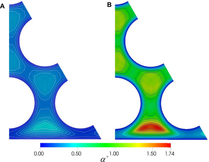
4.3.3 Dimensionless Thermal Diffusivity Distribution

To analyze the dependence of heat transfer on $P{e}_{bun}$, defining the dimensionless thermal diffusivity ${\alpha }^{+}$ as follows:

${\alpha }^{+}=\frac{{\alpha }_t}{\alpha }(27)$

${\alpha }^{+}$ is the ratio between turbulent thermal diffusivity and molecular thermal diffusivity. Figure 8 reports the calculated dimensionless thermal diffusivity distribution on the computational domain for $P{e}_{bun}=500$ and $P{e}_{bun}=1500$. From this figure, it can be clearly seen that the ${\alpha }^{+}$ in the center of each sub-channel is higher than that near the wall, where the heat is mainly derived by the molecular heat conduction. Moreover, in the center of the edge sub-channel $Sub4$, the maximum dimensionless thermal diffusivity can be found, indicating that the thermal diffusion caused by turbulent flow reaches its peak in this region. It should be mentioned that when $P{e}_{bun}=500$, the ${\alpha }^{+}$ in the whole computational domain is less than 1, suggesting that the molecular heat conduction affects the entire computational domain dominantly. In addition, with the increase of $P{e}_{bun}$, a region where turbulent thermal diffusion is stronger than molecular heat conduction begins to appear.

FIGURE 8

FIGURE 8. Dimensionless thermal diffusivity distribution on a computational domain. (A) $P{e}_{bun}=500$ and (B) $P{e}_{bun}=1500.$

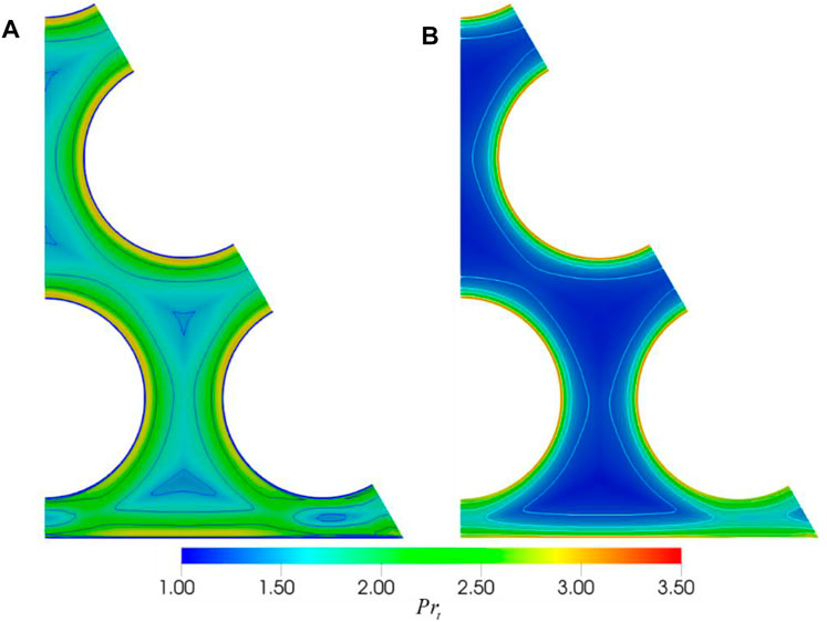
4.3.4 Turbulent Prandtl Number Distribution

The distribution of $P{r}_t$ in the computational domain is plotted against different $P{e}_{bun}$ numbers and displayed in Figure 9. As revealed in this figure, the $P{r}_t$ is higher in the district close to the wall of the heated rod. Moreover, the overall turbulent Prandtl number in the computational domain decreases with the increase of $P{e}_{bun}$. In particular, the turbulent Prandtl number in the turbulent core region decreases significantly with the increase of $P{e}_{bun}$.

FIGURE 9

FIGURE 9. Turbulent Prandtl number distribution on a computational domain. (A) $P{e}_{bun}=1000$ and (B) $P{e}_{bun}=3000.$

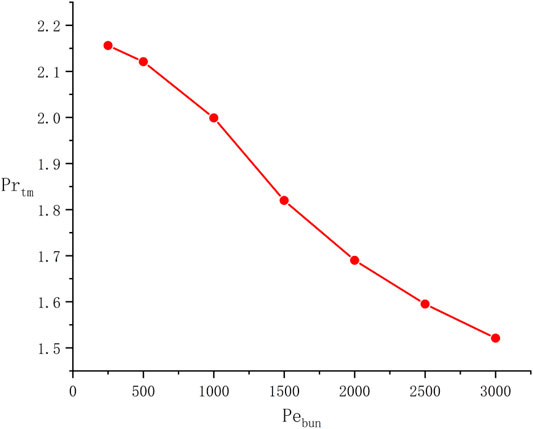
The mean turbulent Prandtl number $P{r}_{tm}$ of the computational domain is defined as follows:

$P{r}_{tm}=\frac{{\displaystyle {\int }_{A}P{r}_{t}dA}}{{\displaystyle {\int }_{A}dA}}(28)$

In order to investigate the influence of $P{e}_{bun}$ on the $P{r}_{tm}$, Figure 10 plots the $P{r}_{tm}$ against different $P{e}_{bun}$. From this figure, it can be concluded that the $P{r}_{tm}$ tends to decrease as the $P{e}_{bun}$ increases. However, the rate of decline also decreases with the increase of $P{e}_{bun}$. Furthermore, the $P{r}_{tm}$ of the computational domain is higher than 1, suggesting that the analogy about $P{r}_t=0.85$ is not appropriate in such low-$Pr$ fluids.

FIGURE 10

FIGURE 10. Mean turbulent Prandtl number of the bare 19-rod bundle.

4.4 Assessment of Different Turbulence Models and Turbulent Heat Transfer Models

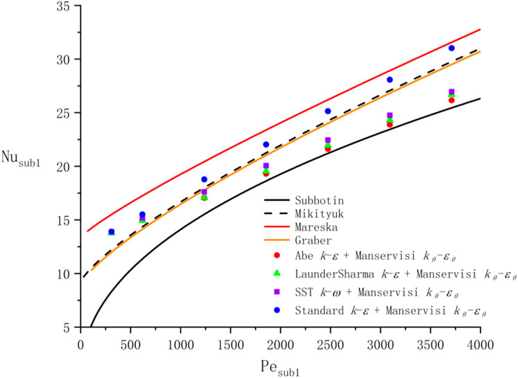
To analyze the effect of the turbulence model on the simulation of heat transfer, in this sub-section, various turbulence models of OpenFOAM are also employed in buoyant2eqnFoam, including standard $k-\epsilon$ (Launder and Spalding, 1972; 1983), SST $k-\omega$ (Menter and Esch, 2001; Menter et al., 2003; Hellsten, 2012), and LaunderSharma $k-\epsilon$ (Launder and Sharma, 1974). The specific definitions of these turbulence models can be found in the literature (Launder and Spalding, 1972; Launder and Sharma, 1974; Launder and Spalding, 1983; Menter and Esch, 2001; Menter et al., 2003; Hellsten, 2012). A comparison of $N{u}_{sub1}$ calculated by different turbulence models with heat transfer experimental correlations is displayed in Figure 11. As demonstrated in this figure, the $N{u}_{sub1}$ calculated by four turbulence models is pretty close when $P{e}_{sub1}<1000$, mainly because the molecular heat conduction is dominant in this Peclet number range. It should be noted, however, that the deviations of $N{u}_{sub1}$ obtained by each turbulence model gradually increase as the Peclet number grows. As indicated in Figure 11, all $N{u}_{sub1}$ predicted by the standard $k-\epsilon$ turbulence model is located between Mareska and Mikityuk correlations. However, for Abe $k-\epsilon$, LaunderSharma $k-\epsilon$, and SST $k-\omega$, the calculated $N{u}_{sub1}$ lies between the Graber and Subbotin correlations when $P{e}_{sub1}>1000$. Although the $N{u}_{sub1}$ results obtained by Abe $k-\epsilon$, LaunderSharma $k-\epsilon$, and SST $k-\omega$ are very similar, in general, Abe $k-\epsilon$ is the most conservative. In addition, the maximum deviation of the Nusselt number obtained by the Abe $k-\epsilon$ and the standard $k-\epsilon$ is close to 19%. It is worth mentioning that due to the significant deviation between the various Nusselt number experimental correlations, the quality of these turbulence models cannot be evaluated. Therefore, great care and caution should be exercised when selecting a turbulence model in simulation. More precise experimental and analytical studies are required in the future to identify the thermohydraulic characteristics of heavy liquid metals like LBE.

FIGURE 11

FIGURE 11. Comparison of $N{u}_{sub1}$ calculated by different turbulence models.

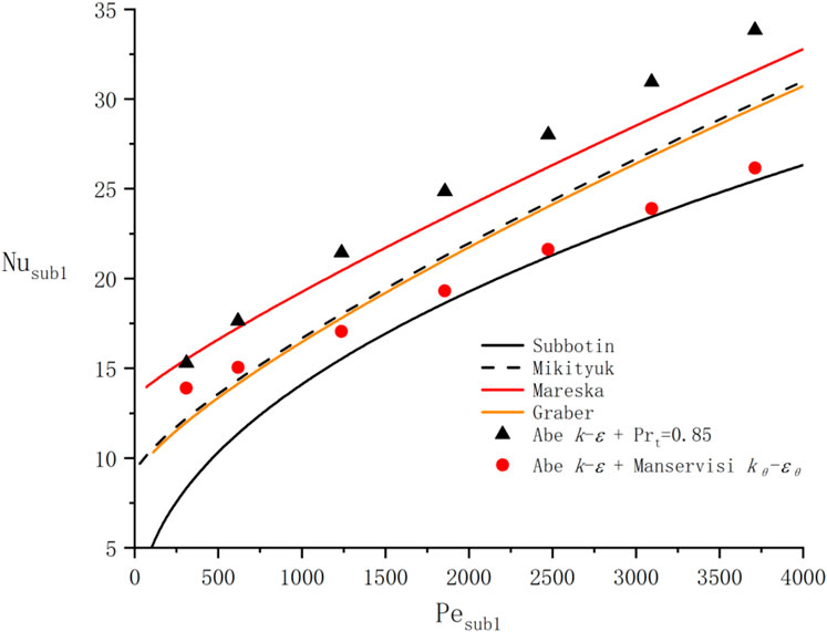
Moreover, the $N{u}_{sub1}$ calculated by the Manservisi $k_{\theta }-{\epsilon }_{\theta }$ model and the $P{r}_t=0.85$ model is reported in Figure 12. It is evident that compared with the experimental correlations plotted in Figure 12, the $N{u}_{sub1}$ obtained by the $P{r}_t=0.85$ heat transfer model is higher under almost all Peclet numbers. Oppositely, the Manservisi $k_{\theta }-{\epsilon }_{\theta }$ heat transfer model provides the more conservative results of $N{u}_{sub1}$.

FIGURE 12

FIGURE 12. Comparison of $N{u}_{sub1}$ calculated by different turbulent heat transfer models.

5 Conclusion

In the current study, the Abe $k-\epsilon$ turbulence model was compiled into the turbulence model library coming with OpenFOAM. A CFD solver buoyant2eqnFoam, which introduces the Manservisi $k_{\theta }-{\epsilon }_{\theta }$ turbulent heat transfer model, was developed. Subsequently, the Abe $k-\epsilon$ turbulence model with wall functions and Manservisi $k_{\theta }-{\epsilon }_{\theta }$ turbulent heat transfer model with zero-gradient boundary were employed to analyze the thermohydraulic characteristics of LBE inner flow in the bare 19-rod bundle. In addition, the influence of the turbulence model on the prediction of turbulent heat transfer was investigated by employing various turbulence models in the self-compiled solver buoyant2eqnFoam, including Abe $k-\epsilon$, standard $k-\epsilon$, SST $k-\omega$, and LaunderSharma $k-\epsilon$. Based on the aforementioned discussions, conclusions obtained from the present work can be summarized as follows:

1) The Nusselt numbers obtained by the self-compiled solver buoyant2eqnFoam are in good agreement with experimental correlations and Chierici simulation research, indicating the validity and reliability of the self-compiled solver.

2) In the bare 19-rod bundle with $P/D=1.4$, the flow resistance of the corner sub-channel is higher than that of other sub-channels due to the smaller hydraulic diameter, leading to the appearance of higher temperature distribution and larger hot spot factor in this region.

3) Although the turbulent Prandtl number of LBE inner flow in the bare 19-rod bundle will decrease as the Peclet number increases, the overall turbulent Prandtl number is higher than 0.85, revealing that the Reynolds-analogy hypothesis about $P{r}_t=0.85$ is not appropriate for low-$Pr$ number fluids like LBE.

4) The turbulence model has a considerable influence on the calculation of turbulent heat transfer of low–$Pr$ number fluids in the high Peclet number range, suggesting that it should be prudent and rigorous when picking a turbulence model in the simulations. Moreover, compared with the $k_{\theta }-{\epsilon }_{\theta }$ turbulent heat transfer model, the Reynolds-analogy hypothesis about $P{r}_t=0.85$ may give the much higher Nusselt numbers in the simulation of low–$Pr$ number fluids.

The applicability of the solver developed in the present study for the more complicated geometry like fuel assembly with grid spacer or wire-wrapped configurations requires further verification.

Data Availability Statement

The original contributions presented in the study are included in the article/supplementary material, further inquiries can be directed to the corresponding authors.

Author Contributions

XL: concept, research, writing, editing, code, and data processing; XS: modification, concept, research, and code; LG: fund, project management, concept, and research; LZ: editing and research; and XS: editing and research.

Funding

This study was supported by the Research on key technology and safety verification of primary circuit, Grant No. 2020YFB1902104; the Experimental study on thermal hydraulics of fuel rod bundle, Grant No. Y828020XZ0; and the National Natural Science Foundation of China, Grant No.12122512.

Conflict of Interest

The authors declare that the research was conducted in the absence of any commercial or financial relationships that could be construed as a potential conflict of interest.

Publisher’s Note

All claims expressed in this article are solely those of the authors and do not necessarily represent those of their affiliated organizations, or those of the publisher, the editors, and the reviewers. Any product that may be evaluated in this article, or claim that may be made by its manufacturer, is not guaranteed or endorsed by the publisher.

References

Abe, K., Kondoh, T., and Nagano, Y. (1994). A New Turbulence Model for Predicting Fluid Flow and Heat Transfer in Separating and Reattaching Flows-I. Flow Field Calculations. Int. J. Heat Mass Transf. 37 (1), 139–151. doi:10.1016/0017-9310(94)90168-6

CrossRef Full Text | Google Scholar

Abram, T., and Ion, S. (2008). Generation-IV Nuclear Power: A Review of the State of the Science. Energy Policy 36 (12), 4323–4330. doi:10.1016/j.enpol.2008.09.059

CrossRef Full Text | Google Scholar

Carteciano, L., Dorr, B., Grötzbach, G., Olbrich, W., and Jin, X. J. F. (2001). Two-and Three-Dimensional Thermal and Fluid-Dynamical Analysis of the Complete MEGAPIE-Module with the Computer Code. FLUTAN 6653, 443–458.

Google Scholar

Carteciano, L. J. H. (1995). Analysis of a Turbulence Model for Buoyant Flows Implemented in the 3d Thermal-Hydraulic Computer Code FLUTAN and Comparison with the Standard Kε-Σt Model. Turbulence 1.

Google Scholar

Carteciano, L. N., and Grötzbach, G. (2003). Validation of Turbulence Models in the Computer Code FLUTAN for a Free Hot Sodium Jet in Different Buoyancy Flow Regimes. ETDEWEB.

Google Scholar

Carteciano, L., Weinberg, D., and Müller, U. (1997). “Development and Analysis of a Turbulence Model for Buoyant Flows,” in Proc. of the 4th World Conf. on Experimental Heat Transfer, Fluid Mechanics and Thermodynamics, Bruxelles, Belgium, 2–6. June: Citeseer).

Google Scholar

Cerroni, D., Da Via, R., Manservisi, S., Menghini, F., Pozzetti, G., and Scardovelli, R. (2015). Numerical Validation of a κ-ω-κθ-ωθ Heat Transfer Turbulence Model for Heavy Liquid Metals. J. Phys. Conf. Ser. 655 (1), 012046. IOP Publishing). doi:10.1088/1742-6596/655/1/012046

CrossRef Full Text | Google Scholar

Cervone, A., Chierici, A., Chirco, L., Da Vià, R., Giovacchini, V., and Manservisi, S. (2020). CFD Simulation of Turbulent Flows over Wire-Wrapped Nuclear Reactor Bundles Using Immersed Boundary Method. J. Phys. Conf. Ser. 1599 (1), 012022. IOP Publishing). doi:10.1088/1742-6596/1599/1/012022

CrossRef Full Text | Google Scholar

Cheng, X., and Tak, N.-I. (2006). Investigation on Turbulent Heat Transfer to Lead-Bismuth Eutectic Flows in Circular Tubes for Nuclear Applications. Nucl. Eng. Des. 236 (4), 385–393. doi:10.1016/j.nucengdes.2005.09.006

CrossRef Full Text | Google Scholar

Chierici, A., Chirco, L., Da Vià, R., and Manservisi, S. (2019). Numerical Simulation of a Turbulent Lead Bismuth Eutectic Flow inside a 19 Pin Nuclear Reactor Bundle with a Four Logarithmic Parameter Turbulence Model. J. Phys. Conf. Ser. 1224 (1), 012030. IOP Publishing). doi:10.1088/1742-6596/1224/1/012030

CrossRef Full Text | Google Scholar

Da Vià, R., Giovacchini, V., and Manservisi, S. (2020). A Logarithmic Turbulent Heat Transfer Model in Applications with Liquid Metals for Pr= 0.01–0.025. Appl. Sci. 10 (12), 4337. doi:10.3390/app10124337

CrossRef Full Text | Google Scholar

Da Vià, R., Manservisi, S., and Menghini, F. (2016). A K-Ω-Kθ-Ωθ Four Parameter Logarithmic Turbulence Model for Liquid Metals. Int. J. Heat Mass Transf. 101, 1030–1041. doi:10.1016/j.ijheatmasstransfer.2016.05.084

CrossRef Full Text | Google Scholar

Da Vià, R., and Manservisi, S. (2019). Numerical Simulation of Forced and Mixed Convection Turbulent Liquid Sodium Flow over a Vertical Backward Facing Step with a Four Parameter Turbulence Model. Int. J. Heat Mass Transf. 135, 591–603. doi:10.1016/j.ijheatmasstransfer.2019.01.129

CrossRef Full Text | Google Scholar

Darwish, M., and Moukalled, F. (2021). The Finite Volume Method in Computational Fluid Dynamics: An Advanced Introduction with OpenFOAM® and Matlab®. Springer.

Google Scholar

De Santis, A., and Shams, A. (2018). Application of an Algebraic Turbulent Heat Flux Model to a Backward Facing Step Flow at Low Prandtl Number. Ann. Nucl. Energy 117, 32–44. doi:10.1016/j.anucene.2018.03.016

CrossRef Full Text | Google Scholar

De Santis, D., De Santis, A., Shams, A., and Kwiatkowski, T. (2018). The Influence of Low Prandtl Numbers on the Turbulent Mixed Convection in an Horizontal Channel Flow: DNS and Assessment of RANS Turbulence Models. Int. J. Heat Mass Transf. 127, 345–358. doi:10.1016/j.ijheatmasstransfer.2018.07.150

CrossRef Full Text | Google Scholar

Deng, B., Wu, W., and Xi, S. (2001). A Near-Wall Two-Equation Heat Transfer Model for Wall Turbulent Flows. Int. J. Heat Mass Transf. 44 (4), 691–698. doi:10.1016/s0017-9310(00)00131-9

CrossRef Full Text | Google Scholar

Ge, Z., Liu, J., Zhao, P., Nie, X., and Ye, M. (2017). Investigation on the Applicability of Turbulent-Prandtl-Number Models in Bare Rod Bundles for Heavy Liquid Metals. Nucl. Eng. Des. 314, 198–206. doi:10.1016/j.nucengdes.2017.01.032

CrossRef Full Text | Google Scholar

Gräber, H., and Rieger, M. J. A. (1972). Experimentelle Untersuchung des Wärmeübergangs an Flüssigmetalle (NaK) in parallel durchströmten Rohrbündeln bei konstanter und exponentieller Wärmeflussdichteverteilung. Atomkernenergie (ATKE) Bd. 19 23-40.

Google Scholar

Gu, L., and Su, X. (2021). Latest Research Progress for LBE Coolant Reactor of China Initiative Accelerator Driven System Project. Front. Energy 15 (4), 810–831. doi:10.1007/s11708-021-0760-1

CrossRef Full Text | Google Scholar

Hanjalić, K., Kenjereš, S., and Durst, F. (1996). Natural Convection in Partitioned Two-Dimensional Enclosures at Higher Rayleigh Numbers. Int. J. Heat Mass Transf. 39 (7), 1407–1427.

Google Scholar

Hattori, H., Nagano, Y., and Tagawa, M. (1993). Analysis of Turbulent Heat Transfer under Various Thermal Conditions with Two-Equation Models. In Engineering Turbulence Modelling and Experiments, 43–52. Elsevier

CrossRef Full Text | Google Scholar

He, S., Wang, M., Zhang, J., Tian, W., Qiu, S., Su, G. H., et al. (2021). Numerical Simulation of Three-Dimensional Flow and Heat Transfer Characteristics of Liquid Lead-Bismuth. Nucl. Eng. Technol. 53 (6), 1834–1845. doi:10.1016/j.net.2020.12.025

CrossRef Full Text | Google Scholar

Hellsten, A. (2012). “Some Improvements in Menter's K-Omega SST Turbulence Model,” in 29th AIAA, Fluid Dynamics Conference, 2554.

Google Scholar

Hwang, C. B., and Lin, C. A. (1999). A Low Reynolds Number Two-Equation Model to Predict Thermal Fields. Int. J. Heat Mass Transf. 42 (17), 3217–3230. doi:10.1016/s0017-9310(98)00382-2

CrossRef Full Text | Google Scholar

Karcz, M., and Badur, J. (2005). An Alternative Two-Equation Turbulent Heat Diffusivity Closure. Int. J. Heat Mass Transf. 48 (10), 2013–2022. doi:10.1016/j.ijheatmasstransfer.2004.12.006

CrossRef Full Text | Google Scholar

Kawamura, H., Abe, H., Matsuo, Y., and Flow, F. (1999). DNS of Turbulent Heat Transfer in Channel Flow with Respect to Reynolds and Prandtl Number Effects. Int. J. Heat Fluid Flow 20 (3), 196–207. doi:10.1016/s0142-727x(99)00014-4

CrossRef Full Text | Google Scholar

Kenjereš, S., Gunarjo, S., and Hanjalić, K. (2005). Contribution to Elliptic Relaxation Modelling of Turbulent Natural and Mixed Convection. Int. J. Heat Fluid Flow 26 (4), 569–586.

Google Scholar

Launder, B. E., and Sharma, B. I. (1974). Application of the Energy-Dissipation Model of Turbulence to the Calculation of Flow Near a Spinning Disc. Lett. Heat Mass Transf. 1 (2), 131–137. doi:10.1016/0094-4548(74)90150-7

CrossRef Full Text | Google Scholar

Launder, B. E., and Spalding, D. B. (1972). Lectures in Mathematical Models of Turbulence. Academic Press.

Google Scholar

Launder, B. E., and Spalding, D. B. (1983). “The Numerical Computation of Turbulent Flows,” in Numerical Prediction of Flow, Heat Transfer, Turbulence and Combustion (Elsevier), 96–116. doi:10.1016/b978-0-08-030937-8.50016-7

CrossRef Full Text | Google Scholar

Manservisi, S., and Menghini, F. (2014a). A CFD Four Parameter Heat Transfer Turbulence Model for Engineering Applications in Heavy Liquid Metals. Int. J. Heat Mass Transf. 69, 312–326. doi:10.1016/j.ijheatmasstransfer.2013.10.017

CrossRef Full Text | Google Scholar

Manservisi, S., and Menghini, F. (2015). CFD Simulations in Heavy Liquid Metal Flows for Square Lattice Bare Rod Bundle Geometries with a Four Parameter Heat Transfer Turbulence Model. Nucl. Eng. Des. 295, 251–260. doi:10.1016/j.nucengdes.2015.10.006

CrossRef Full Text | Google Scholar

Manservisi, S., and Menghini, F. (2014b). Triangular Rod Bundle Simulations of a CFD κ-ϵ-κ-ϵ Heat Transfer Turbulence Model for Heavy Liquid Metals. Nucl. Eng. Des. 273, 251–270. doi:10.1016/j.nucengdes.2014.03.022

CrossRef Full Text | Google Scholar

Mareska, M. W., and Dwyer, O. E. (1964). Heat Transfer in a Mercury Flow along Bundles of Cylindrical Rods. J. Heat. Transf. 86 (2), 180–186.)

Google Scholar

Martelli, D., Marinari, R., Barone, G., Di Piazza, I., and Tarantino, M. (2017). CFD Thermo-Hydraulic Analysis of the CIRCE Fuel Bundle. Ann. Nucl. Energy 103, 294–305. doi:10.1016/j.anucene.2017.01.031

CrossRef Full Text | Google Scholar

Menter, F., and Esch, T. (2001). “Elements of Industrial Heat Transfer Predictions,” in 16th Brazilian Congress of Mechanical Engineering (COBEM), 650.

Google Scholar

Menter, F. R., Kuntz, M., and Langtry, R. J. T. (2003). Ten Years of Industrial Experience with the SST Turbulence Model. Heat Mass Transf. 4 (1), 625–632.

Google Scholar

Mikityuk, K. (2009). Heat Transfer to Liquid Metal: Review of Data and Correlations for Tube Bundles. Nucl. Eng. Des. 239 (4), 680–687. doi:10.1016/j.nucengdes.2008.12.014

CrossRef Full Text | Google Scholar

Nagano, Y., Hattori, H., and Abe, K. (1997). Modeling the Turbulent Heat and Momentum Transfer in Flows under Different Thermal Conditions. Fluid Dyn. Res. 20 (1-6), 127–142. doi:10.1016/s0169-5983(96)00049-4

CrossRef Full Text | Google Scholar

Nagano, Y., and Kim, C. (1988). A Two-Equation Model for Heat Transport in Wall Turbulent Shear Flows. J. Heat. Transf. 110 (3), 583–589. doi:10.1115/1.3250532

CrossRef Full Text | Google Scholar

Nagano, Y. (2002). Modelling Heat Transfer in Near-Wall Flows, 188–247.

Google Scholar

Nagano, Y., and Shimada, M. (1996). Development of a Two‐equation Heat Transfer Model Based on Direct Simulations of Turbulent Flows with Different Prandtl Numbers. Phys. Fluids 8 (12), 3379–3402. doi:10.1063/1.869124

CrossRef Full Text | Google Scholar

Otić, I., and Grötzbach, G. (2007). Turbulent Heat Flux and Temperature Variance Dissipation Rate in Natural Convection in Lead-Bismuth. Nucl. Sci. Eng. 155 (3), 489–496.

Google Scholar

Otić, I., Grötzbach, G., and Wörner, M. (2005). Analysis and Modelling of the Temperature Variance Equation in Turbulent Natural Convection for Low-Prandtl-Number Fluids. J. Fluid Mech. 525, 237–261.

Google Scholar

Pacio, J., Daubner, M., Fellmoser, F., Litfin, K., Marocco, L., Stieglitz, R., et al. (2014). Heavy-liquid Metal Heat Transfer Experiment in a 19-rod Bundle with Grid Spacers. Nucl. Eng. Des. 273, 33–46. doi:10.1016/j.nucengdes.2014.02.020

CrossRef Full Text | Google Scholar

Pacio, J., Litfin, K., Batta, A., Viellieber, M., Class, A., Doolaard, H., et al. (2015). Heat Transfer to Liquid Metals in a Hexagonal Rod Bundle with Grid Spacers: Experimental and Simulation Results. Nucl. Eng. Des. 290, 27–39. doi:10.1016/j.nucengdes.2014.11.001

CrossRef Full Text | Google Scholar

Pacio, J., Wetzel, T., Doolaard, H., Roelofs, F., and Van Tichelen, K. (2017). Thermal-hydraulic Study of the LBE-Cooled Fuel Assembly in the MYRRHA Reactor: Experiments and Simulations. Nucl. Eng. Des. 312, 327–337. doi:10.1016/j.nucengdes.2016.08.023

CrossRef Full Text | Google Scholar

Shams, A., Mikuž, B., and Roelofs, F. (2018). Numerical Prediction of Flow and Heat Transfer in a Loosely Spaced Bare Rod Bundle. Int. J. Heat Fluid Flow 73, 42–62. doi:10.1016/j.ijheatfluidflow.2018.07.006

CrossRef Full Text | Google Scholar

Shams, A., Roelofs, F., Baglietto, E., Lardeau, S., and Kenjeres, S. (2014). Assessment and Calibration of an Algebraic Turbulent Heat Flux Model for Low-Prandtl Fluids. Int. J. Heat Mass Transf. 79, 589–601. doi:10.1016/j.ijheatmasstransfer.2014.08.018

CrossRef Full Text | Google Scholar

Shams, A. (2018). Towards the Accurate Numerical Prediction of Thermal Hydraulic Phenomena in Corium Pools. Ann. Nucl. Energy 117, 234–246. doi:10.1016/j.anucene.2018.03.031

CrossRef Full Text | Google Scholar

Shin, J. K., An, J. S., Choi, Y. D., Kim, Y. C., and Kim, M. S. (2008). Elliptic Relaxation Second Moment Closure for the Turbulent Heat Fluxes. J. Turbul. 9 (9), N3. doi:10.1080/14685240701823101

CrossRef Full Text | Google Scholar

Simcenter, (2016). STAR-CCM+ Documentation.

Google Scholar

Sommer, T. P., So, R. M. C., and Lai, Y. G. (1992). A Near-Wall Two-Equation Model for Turbulent Heat Fluxes. Int. J. Heat Mass Transf. 35 (12), 3375–3387. doi:10.1016/0017-9310(92)90224-g

CrossRef Full Text | Google Scholar

Su, X., Li, X., Wang, X., Liu, Y., Chen, Q., Shi, Q., et al. (2022). Development and Assessment of an Isotropic Four-Equation Model for Heat Transfer of Low Prandtl Number Fluids. Front. Energy Res. 57. doi:10.3389/fenrg.2022.816560

CrossRef Full Text | Google Scholar

Subbotin, V., Ushakov, P., Kirillov, P., Ibragimov, M., Ivanovski, M., Nomofilov, E., et al. (1965). “Heat Transfer in Elements of Reactors with a Liquid Metal Coolant,” in Proceedings of the 3rd International Conference on Peaceful Use of Nuclear Energy, 192–200.

Google Scholar

Youssef, M. S. (2006). A Two-Equation Heat Transfer Model for Wall Turbulent Shear Flows. JES. J. Eng. Sci. 34 (6), 1877–1903. doi:10.21608/jesaun.2006.111184

CrossRef Full Text | Google Scholar

Youssef, M. S., Nagano, Y., and Tagawa, M. (1992). A Two-Equation Heat Transfer Model for Predicting Turbulent Thermal Fields under Arbitrary Wall Thermal Conditions. Int. J. Heat Mass Transf. 35 (11), 3095–3104. doi:10.1016/0017-9310(92)90329-q

CrossRef Full Text | Google Scholar