 Yan Ren1,2*
 Ruoyu Qiao
- 1School of Electric Power, North China University of Water Resources and Electric Power, Zhengzhou, China
- 2Yellow River Engineering Consulting Co., Ltd., Zhengzhou, China
Wind and photovoltaic (PV) power generation and other distributed energy sources are developing rapidly. But due to the influence of the environment and climate, the output is very unstable, which affects the power quality and power system stability. Pumped hydroelectric energy storage (PHES) systems are suitable as peaking power sources for wind and photovoltaic (Wind–PV) complementary systems because of their fast start–stop and long life. The mathematical models and operational characteristics of the three subsystems in the wind–PV–PHES complementary system are analyzed to improve the generation efficiency and access capacity of wind and PV power. The peaking characteristics of the PHES system are used to balance the maximum benefit and minimum output fluctuation of the wind–PV complementary system. The stable operation of the pump turbine is an important guarantee for the smooth output of the wind–PV complementary system. Three operating points are selected from the net load curve and converted to the pump turbine model parameters. The internal flow characteristics and laws of the pump turbine under different guide vane opening conditions are summarized through the analysis of the computational fluid dynamics (CFD) numerical simulation post-processing results. The study shows that the output of wind and PV power generation varies with the changes in wind speed and solar radiation, respectively. The output of the wind–PV complementary system still has large fluctuations, and the PHES system can effectively suppress the power fluctuation of the wind–PV complementary system and reduce the abandoned wind and light rate. CFD technology can accurately and efficiently characterize the internal flow characteristics of the pump turbine, which provides a basis for the design, optimization, and transformation of the pump turbine.
1 Introduction
Currently, the world’s energy landscape is undergoing profound changes; in this context, countries around the world are scrambling to find ways to transform energy, and actively develop clean energy sources such as solar energy, hydro energy, nuclear energy, wind energy, and tidal energy to gradually replace the fossil energy. However, with rapid economic development, energy demand is increasing, environmental issues are becoming increasingly prominent, and the traditional energy structure is difficult to support sustainable development. Therefore, it is necessary to take a green and low-carbon path to ensure energy security. With the development and utilization of wind power (Dowds et al., 2015), PV power generation can greatly alleviate the problem of electricity tension and energy depletion.
Wind power (Zhang and Qi, 2011) and PV power (Zhang et al., 2021) generation has the advantages of good environmental benefits, and clean and renewable energy. At the same time, wind power and PV power generation is volatile, random (Abadi and El-Saadany, 2010), and intermittent (Ren et al., 2017). In addition, it is difficult to store them, which results in high operation and maintenance costs. Electric energy can be converted into many other forms of energy for storage (Koohi-Fayegh and Rosen, 2020), such as kinetic energy in the impeller, electric field in the capacitor, gravitational potential energy in the reservoir, electrochemical energy, and chemical energy in the fuel cell. Barra et al. (2021) discussed and compared energy storage technologies and provided a comprehensive review of important research on wind power smoothing using these storage systems. Wu et al. (2014) and Acu ñ a et al. (2018) connected the battery storage device to the wind–PV power system and studied the optimal scheduling and capacity allocation of the wind–PV–battery system to maximize the use of renewable energy. Conventional battery storage cannot be used in large-scale practical scenarios due to cost, environmental requirements, safety, and lifetime limitations. Pumped storage energy plants can be used as storage power sources because of their stability and large capacity as physical energy storage. Considering the intermittent nature of solar and wind energy and the variation in load demand, Kusakana (2016) created an energy dispatch model to meet the load demand; the main objective of the model was to provide a multi-energy complementary system composed of PV, wind (Parastegari et al., 2015), PHES, and diesel generators. The main goal was to reduce the operating costs of the system within the operating limits of the different components and optimize the stability of the system. When designing a multi-energy complementary system, cost and reliability are prerequisites and foundations, while also considering the demand-side response. Xu et al. (2020) designed a PV–wind–PHES complementary system from an investor’s perspective using various algorithms to find the optimal configuration with maximum power supply reliability and minimum investment cost. Jurasz (2017) combined a mixed-integer model with an artificial neural network prediction method to predict the amount of energy flow between a local balancing area using a PV–wind–PHES complementary system and the national power system. Rathore and Patidar (2019) evaluated the reliability of a PHES system under a wind–PV–PHES complementary system based on metrics such as load expectation and expected energy not served. After comparison, the PHES system was found to be more reliable and environmentally friendly than battery storage systems. PHES systems are being widely used to overcome the economic and environmental disadvantages of electrochemical energy storage devices.
The PHES (Gao et al., 2018; Wu et al., 2020) technology is mature, with the advantages of flexible start-up, fast climbing and unloading, peak and valley regulation, frequency regulation, etc. It can well mitigate the adverse effects of distributed energy sources such as PV power generation and wind power generation on the power system and maintain the stable operation of the power system. Archimedes pump (Waters and Aggidis, 2015) is one of the oldest engineering masterpieces, with a history of more than 2000 years, and is still in use today. Since the last century, it has been significantly developed in modern engineering and can be reversed to be used as a turbine, known as a pump turbine (Bogdanovic-Jovanovic et al., 2014; Li et al., 2019) used to explore the internal flow pattern and equipment performance of the pump turbine in a cost-effective manner. Reversible pump turbines are widely used in the power market because they can switch between pump and turbine operation in a matter of minutes. The operating characteristics of a pump turbine are related to the geometry of the flow path. Olimstad et al. (2012) composed several scenarios for computational fluid dynamics (CFD) numerical simulation by varying the angle and radius of curvature of the blade inlet, and found that the unstable pump turbine characteristics are the result of vortex formation in the runner and guide vane channels, with leading edges having a longer radius of curvature that is more prone to vortex formation. The stability of the pump turbine (Zuo and Liu, 2017) is very important for the operation of the PHES system, and unstable characteristics can lead to hazards for the operation of the unit. Widmer et al. (2011) used a combination of CFD numerical simulations and test bench measurements to analyze the mechanisms of vortex formation and rotational stall caused by the turbine model of the pump turbine. Barrio et al. (2011) performed a series of complementary experimental measurements from the test bench to obtain the general characteristics of the pump condition and turbine condition to verify the correctness of the numerical simulation results. The post-processing results were used to investigate the flow regime at some important locations by utilizing pressure and velocity contours and vector plots.
In summary, the current research on wind–PV–PHES complementary systems (Dianellou et al., 2021) only involves capacity allocation (Xu et al., 2019) and scheduling optimization (Zare Oskouei and Sadeghi Yazdankhah, 2015). Most of the studies on the characteristics of pumped turbines have been carried out in the context of traditional PHES technology. In this article, the research is divided into two parts: one is to study the output characteristics of the complementary system and its two subsystems with a given capacity configuration and the other is to conduct CFD numerical simulations of the typical working conditions of the pump turbine in the complementary system with different guide vane openings to investigate its flow characteristics. The main contributions are as follows:
1) analyze operational characteristics of wind and PV power systems of defined capacity;
2) analyze the wind–PV complementary system (Sinha and Chandel, 2015) and the operating characteristics of the wind–PV–PHES complementary system after adding typical loads to obtain the net load curve; and
3) select three prototype operating points from the net load curve and convert them to the relevant parameters of the model pump turbine. The CFD numerical simulation is carried out to analyze the flow characteristics inside the pump turbine under the wind–PV–PHES complementary system.
The remaining sections of this article are organized as follows. In Chapter 2, a three-dimensional model of the pump turbine is established, and the meshing and irrelevance are verified. The output mathematical models of wind power, PV power, and PHES systems are established. In Chapter 3, the output characteristics of the aforementioned systems are analyzed, and on this basis, the operating characteristics of the wind–PV system and the wind–PV–PHES system with three typical loads are analyzed and the net load curves are drawn. In Chapter 4, three prototype operating points are selected from the net load curves in Chapter 3 and reflected from the comprehensive characteristic curves of the pump turbine model after conversion. CFD numerical simulations are performed for the three selected operating points with different guide vane openings. The laws and characteristics of the internal flow state of the pump turbine are summarized after analysis of the post-processing results. Chapter 5 is a summary of the research findings. The workflow of this article is shown in Figure 1.
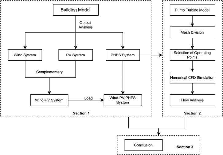
FIGURE 1. Workflow diagram.
2 Methods and Mathematical Models
2.1 Methods
2.1.1 CFD Numerical Simulation Method
CFD technology can be understood as a numerical simulation method of flow controlled by the fundamental flow equations (conservation of mass, conservation of momentum, and conservation of energy). The distribution of basic physical quantities, such as velocity, pressure, temperature, and concentration, at different locations in the flow field and the variation in these physical quantities with time can be obtained by numerical simulation. Then the vortex distribution characteristics, cavitation characteristics, and delocalization zone can be observed. Therefore, CFD can be used not only for flow field analysis but also for further study of the fluid flow mechanism inside the pump turbine (Tao and Wang, 2021) and the transition process (Wang et al., 2011). At the same time, it can be used as a tool to calculate the external performance parameters such as the head and shaft power of the pump turbine. In addition, combined with CAD software, it can also optimize the design of the structure.
However, the flow characteristics inside most hydraulic machines are difficult to be studied by building test benches due to the limitations of funding, space, accuracy, and time and labor costs. Therefore, the use of CFD numerical simulation to study fluid problems is a proven method. However, the traditional calculation method has many drawbacks: it requires a lot of mathematical derivation, and the solution process is complicated and time-consuming. Therefore, it is difficult to meet the requirements of engineering practice. The aforementioned disadvantages of the CFD numerical simulation method can be overcome by exploring the internal flow characteristics of the hydraulic machinery with the help of computer resources. For example, the CFD numerical simulation method can be used to understand in detail the flow in the pump turbine pipeline, the formation and propagation of vortices, pressure distribution, flow velocity distribution, force magnitude, and its change with time.
2.1.2 Flow Control Equation
The flow in a pump turbine, regardless of the flow rate, is always governed by the basic physical conservation laws. The corresponding control equations are as follows.
Continuous Equation:
where
Momentum Equation:
where
Energy Equation:
where
2.1.3 Establishment of the Three-Dimensional Model of the Pump Turbine
The pump turbine of a PHES system is chosen as the object of calculation, and the main basic parameters are shown in Table 1.
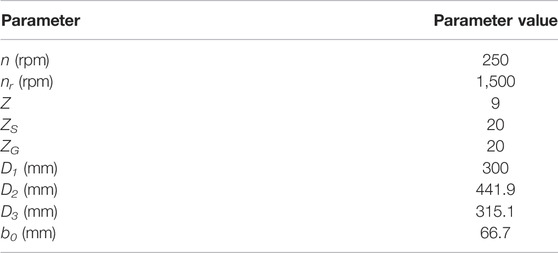
TABLE 1. Basic parameters of the pump turbine of a pumped storage power station.
The overflow components such as the stay vane, guide vane, volute, runner, and draft tube are modeled in the fluid domain using Unigraphics NX software, and then assembled as shown in Figure 2.
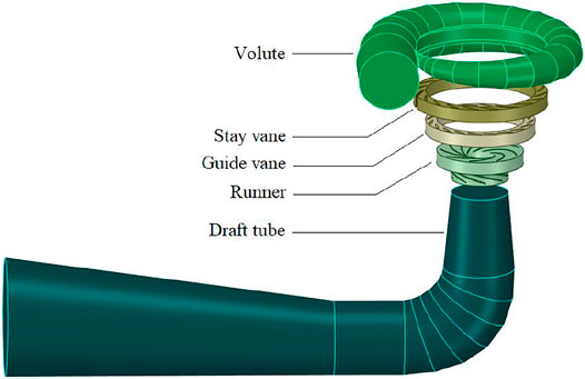
FIGURE 2. Full flow channel three-dimensional hydraulic model of the pump turbine.
Since the modeling idea of the full flow channel 3D hydraulic model of the pump turbine is to build each overflow component separately and then assemble it, the internal flow field between two adjacent components cannot be connected when using Fluent for CFD numerical simulation. Therefore, to realize the connection of the whole flow field, the common practice is to create interface surfaces between the components. The Shared Topology function in ANSYS SpaceClaim can automatically identify the contacting or intersecting bodies and share their topology, replacing the complicated setting of interface surfaces. The schematic diagram is shown in Figure 3.
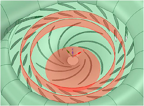
FIGURE 3. Shared topology schematic.
2.1.4 Pump Turbine Meshing and Mesh Irrelevance Verification
To ensure the solution accuracy and time, and to take into account the computer resources, Poly-Hexcore mesh, which consists of laminated polyhedra mesh, pure polyhedra mesh, and hexahedra mesh (Hexcore), is used for meshing the pump turbine 3D model.
The grid-independence test requires that the sparsity of the grid has as little effect as possible on the results of CFD numerical simulations. But the number of grids can be increased to improve the computational accuracy under the condition that sufficient computational resources are available. The former is widely used because of its high efficiency, while the latter is difficult to be widely used because of its inherent large errors and difficulties. Since the grid has many influencing factors besides model accuracy, such as model boundary conditions and residual criteria, increasing the number of grids may not necessarily improve the accuracy of the calculation. But if the number of grids is so small that it cannot represent the complete details of the model, it will be impossible to obtain more accurate calculation results.
In general, the larger the number of grids, the higher the computational accuracy, and the larger the number of grids, the greater the pressure on the computational resources. Therefore, while ensuring computational accuracy, the pressure on computational resources should be taken into account. For the verification of the grid-independence under optimal operating conditions in the hydraulic turbine mode of the pump turbine, five groups of different numbers of grids are divided in the range of 1–4.5 million for numerical calculation. The relative errors of the head and efficiency calculated by numerical calculation and the experimental values are shown in Figure 4. As can be seen from Figure 4, the two curves represent the relative errors between the numerical simulation results and the experimental values for different grid number scenarios for the head and efficiency, respectively. The relative error reaches the minimum when the number of grid cells is 2,797,995, and the error is maintained within 2% to meet the calculation requirements, after which the relative error increases slightly again with the increase in the number of grid cells.
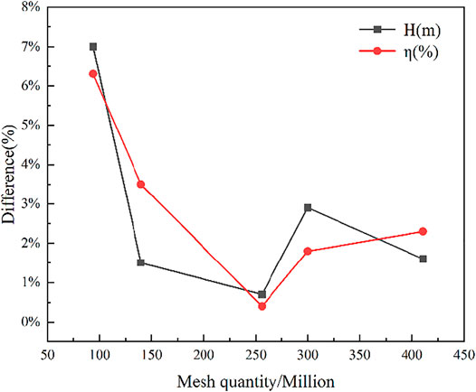
FIGURE 4. Schematic diagram of grid independence verification.
Taking into account the computational resources and computational accuracy, the final number of grid cells is determined to be 2,797,995. The number of grid cells of each component is shown in Table 2, and the schematic diagram of grid division is shown in Figure 5. As can be seen from Figure 5, the surface of the mesh is roughly honeycomb-shaped, and the interior is filled with positive hexahedra. The regularity of each cell is high, and the connectivity between cells is excellent. There will be different degrees of encryption in the transition area between the lower curvature, complex structure, and adjacent two parts.

TABLE 2. Number of grid cells for each component.
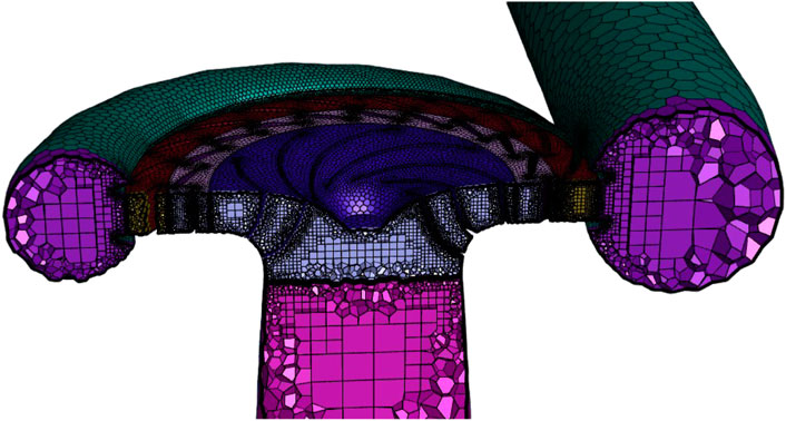
FIGURE 5. Schematic diagram of grid division.
2.2 Mathematical Models
The wind–PV–PHES complementary system is an important type of multi-energy complementary power generation system that can well integrate distributed energy sources, reduce the abandoned wind and light rate, and improve power quality. The wind–PV–PHES complementary system consists of three subsystems: PHES system, wind, and PV power system.
2.2.1 Wind Power Generation
For wind turbines, their output is strongly related to the local wind speed; especially the wind speed at the height of the rotor determines the output. But since the wind speed at the height of the rotor is difficult to measure, the wind speed at the ground level needs to be converted according to the empirical formula.
where
For a specific wind turbine, the power curve shows the relationship between the wind speed and the generator output. Figure 6 shows the power curve of a typical wind turbine with a quadratic approximation. The corresponding output expression is given by the following equation.
where
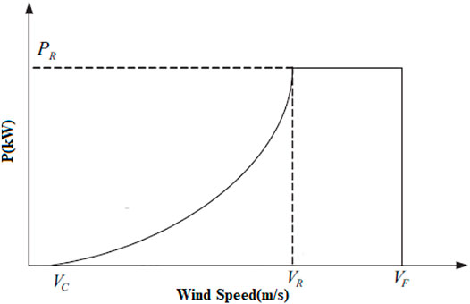
FIGURE 6. Power curve of the wind turbine.
2.2.2 Mathematical Model of PV Power Generation
Solar radiation and ambient temperature will have a direct impact on the output of PV power generation, and its output mathematical model is shown as follows:
where
where
Under the influence of solar radiation absorption and ambient temperature, the temperature of the PV module changes as follows:
where
2.2.3 Mathematical Model of the Pumped Storage Unit
The PHES system mainly consists of an upper reservoir, lower reservoir, transmission pipeline, and plant. The reversible pump turbine is the core component of the PHES system, which realizes pumping and power generation functions through working condition conversion.
When the pump turbine is in stable operation, for an ideal viscosity-free fluid, the work carried out by the water flow on the runner is as follows:
where
Under the turbine model, the output transmitted from the shaft end of the main shaft to the generator is called the output of the turbine.
where
Under the pump model, the energy of the water flow through the pump per unit time is called the effective power.
Then the power transmitted by the motor to the shaft end of the pump, that is, the shaft power, is as follows:
where
3 Result and Discussion
3.1 Characterization
PV and wind power have some complementary characteristics. When the sunshine is abundant during the day, the PV generator sets have a high output and generation, while the wind generator sets have a relatively low power generation due to the reduction of wind speed on sunny days. When there is no light at night, there is no PV power output and PV power generation is 0, while wind power usually has a high wind speed at night, and the output increases and the power generation increases. At this time, the PHES system can be operated under pumping or power generation conditions according to the size of the load in the system and the real-time output of the wind–PV complementary system, so as to play the role of peak and valley regulation and suppress the fluctuation of output in the whole system, and then improve the power quality and the energy utilization rate.
The PHES system runs pumping conditions when the grid load is low to pump water to the reservoir, and then converts under turbine condition when the grid load is high to generate electricity to meet the demand of the grid. It can play a multi-role function of source, load, and storage in ensuring the balance of supply and demand of the grid operation, with the characteristics of fast start-up, fast response, and outstanding peak and valley regulation. This can effectively improve the intermittent, fluctuating, and random nature of wind and PV power generation, maintain the balance of supply and demand in the grid, and enhance the resilience of power security.
The installed capacity of each subsystem in this article is set as follows: 300 MW for the PHES subsystem with two units, 600 MW for the PV power subsystem, and 800 MW for the wind power subsystem, which is based on the operational characteristics of each subsystem and the principle of not wasting installed resources. Taking into account the actual power generation characteristics of wind power and PV power, the wind, PV, and PHES subsystems and the power load in a 24-h cycle are studied, and the power generation characteristics of the subsystems themselves, the wind–PV complementary system, and the multi-energy complementary systems after adding the PHES system are analyzed.
3.1.1 Analysis of Wind Power System Characteristics
The fundamental reason for the large fluctuation of wind power is the natural intermittency and random fluctuation of wind energy resources. The wind speed is affected by a variety of complex natural factors such as climate, weather, and terrain. The wind power system output characteristics of a typical year are shown in Figure 7. It can be seen from the figure that the wind power system output is random and irregular during 8,760 h. It is known that the total installed capacity of wind power is 800 MW. In this typical year, the power generation hours with an output range of 0–300 MW, 300–600 MW, and 600–800 MW are 6781, 1069, and 910 h, respectively, accounting for 77.4, 12.2, and 10.4% of 8,760 h in a year after statistics.
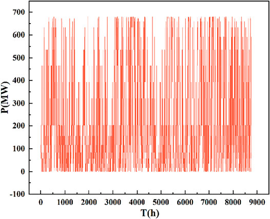
FIGURE 7. Power output characteristics of a typical year wind power system.
From the wind power data of this typical year, three typical days of a strong windy day (SWD), normal windy day (NWD), and weak windy day (WWD) were selected. Their output and wind speed values are listed in Supplementary Table S1, and the output and wind speed distribution of each typical day are plotted as shown in Figure 8.
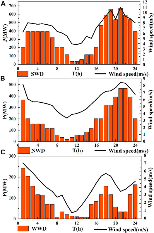
FIGURE 8. Typical daily output and wind speed distribution. (A) SWD, (B) NWD, and (C) WWD.
From the wind power output and wind speed distribution on SWD shown in Figure 8A, it can be seen that wind speed and output fluctuate greatly during the day. The output of wind power on SWD peaks at 21:00 with 672.37 MW, accounting for 84.05% of the installed capacity of the system, and the trough of output is 34.9 MW around 12:00, accounting for 4.36% of the installed capacity of the system. The overall wind speed from 0:00 to 24:00 shows a trend of decreasing first and then increasing. The wind speed fluctuates with time, the minimum wind speed is 3.77 m/s at noon, the wind speed is larger at night, and the output changes with the change in wind speed.
As shown in Figure 8B, the wind power output and wind speed distribution on NWD are similar to those on SWD but fluctuate slightly less than those on SWD. The wind power output peaks at 466.59 MW around 22:00, accounting for 58.32% of the installed capacity of the system and 69.39% of the peak output on SWD. The overall wind speed from 0:00 to 24:00 shows a trend of decreasing first and then increasing. The wind speed fluctuates with time, the minimum wind speed is 3.40 m/s at 11:00, the wind speed is larger at night, and the output changes with the change in wind speed.
From Figure 8C, the wind power output and wind speed distribution on WWD, it can be seen that the trend of wind power output and wind speed is consistent with the other two typical days as a whole. It fluctuates the most among the three typical days and decreases sharply at 21:00–23:00. The overall output value is smaller in a day, the wind power output on SWD peaks at around 00:00 at 241.96 MW, accounting for 30.25% of the system installed capacity and 35.99% of the peak output on SWD. The trough of output is 6.53 MW around 13:00, which is 0.8% of the installed capacity of the system and 18.7% of the trough on SWD. The wind speed is small and fluctuates widely throughout the day, and the minimum wind speed is 0.79 m/s at 11:00.
We analyzed the wind power system output characteristics on three typical days and found that the size of the output varies with the wind speed. The wind speed is low at noon because the sunlight is sufficient at noon, so the output of all three typical days reaches a low point at noon. The wind speed is higher at night, so the output is also higher.
3.1.2 Analysis of PV Power System Characteristics
The difference between PV power and wind power is that it is intermittent and regular. The output is somewhat random and fluctuates due to the influence of weather, season, and sunlight. The PV power system output characteristics of a typical year is shown in Figure 9. From the figure, it can be seen that the PV power system intermittents are greater at 8,760 h. Electricity is generated only in the daytime when there is light; at night when there is no light radiation, no electricity is generated. The output in winter is higher, although the light is longer and irradiance is higher in summer. But the temperature is also high, and high temperature has a significant negative impact on the output of the PV power system, making the overall output in summer lower. The total installed capacity of the PV power system is known to be 600 MW. In this typical year, the number of power generation hours with the output range of 0–200 MW is 6725 h, which is the highest in the year, accounting for 76.8% of the year. The number of power generation hours with the output range of 400–600 MW is 375 h, which is the lowest in the year, accounting for 4.2% of the year.
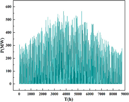
FIGURE 9. Output characteristics of a typical year PV power system.
The output and solar irradiation intensity values are listed in Supplementary Table 2 for the three typical days of sunny day (SD), cloudy day (CD), and rainy day (RD) selected from the typical annual PV power generation data. The output and solar irradiation intensity distribution of each typical day are plotted as shown in Figure 10.
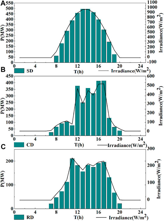
FIGURE 10. Typical daily output and solar irradiation intensity distribution. (A) SD, (B) CD, and (C) RD.
From Figure 10A, the distribution of PV power output and solar irradiation intensity on SD, it can be seen that the PV power system is mainly affected by solar radiation. The solar irradiation and output are approximately normally distributed on SD. As time goes by, the system power gradually increases, reaching a peak at noon and decreasing from afternoon until the sun sets. The solar irradiation appears at around 8:00 and disappears at around 20:00. The solar irradiation reaches a peak of 973 W/m2 at 14:00, and the output value reaches a peak of 496.23 MW at 14:00, accounting for 82.71% of the installed capacity of the system.
From Figure 10B, the distribution of PV power output and solar irradiation intensity on CD, it can be seen that the solar irradiance curve of the PV power system fluctuates more drastically. This leads to higher output volatility and lower output throughout the day, with a large gap between each hour. The solar irradiation appears at around 7:00 and disappears at around 20:00. The solar irradiation reaches a peak of 517 W/m2 at 17:00, and the output value reaches a peak of 415.5 MW at around 17:00, accounting for 69.25% of the installed capacity of the system. The discontinuities are more obvious, with no similar characteristics or clear rules.
From Figure 10C, the distribution of PV power output and solar irradiation intensity on RD, it can be seen that the solar irradiance curve of the PV power system fluctuates more drastically. The output has the characteristics of small output and great fluctuation. The output of the whole day is obviously reduced and is the lowest among the three typical days. The solar irradiance appears at around 7:00 and disappears at around 20:00. The solar irradiation reaches a peak of 250 W/m2 at 11:00, and the output value reaches a peak of 211.25 MW at around 11:00, accounting for 35.21% of the installed capacity of the system.
This section analyzes the output characteristics of the PV power system on three typical days and finds that the output varies with solar irradiance. The output of the PV power system is cyclical 24 h a day, and the output on SD is approximately normally distributed, with a relatively smooth curve. However, the output on RD and CD fluctuates greatly, showing multi-peak characteristics, and there is no specific rule to follow.
3.1.3 Analysis of PHES System Characteristics
Due to the randomness and instability of wind and PV power systems, the PHES system plays the role of peak and valley regulation in the wind–PV complementary system. By working reciprocally to balance the output of wind–PV complementary systems and reduce the rate of wind and light abandonment through the conversion of pumping and power generation conditions. The daily operation diagram of a PHES system for regulating the output of the wind–PV complementary system is shown in Figure 11. From the figure, it can be seen that in the complementary power system containing wind and PV generating units, the net load in the system fluctuates greatly (the size of the net load is the difference between the load in the system and the output of the wind–PV system), and the output of the PHES system changes with the fluctuation of the net load.
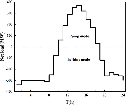
FIGURE 11. Daily operation diagram of a pumped storage power station for regulating the output of the wind–PV complementary system.
During 00:00–7:00, the local wind speed is high, and the wind power system output is also high, while the power system is in the low peak period, so the load is small. To reduce the abandoned wind rate, the PHES system uses the surplus electricity in the complementary system to pump the water to the upper reservoir under the pump mode to store the potential energy for peak regulation. During 9:00–18:00, with the significant increase in the complementary system load, the PHES system will release the water stored in the upper reservoir to the lower reservoir and generate electricity under the turbine mode to supply the load to fill the valley.
3.1.4 Analysis of Wind–PV Complementary System Characteristics
The output of the wind–PV power system has certain complementary characteristics. So in order to reduce the rate of wind and light abandonment and the fluctuation of system output, the wind and PV power systems are coupled by using the natural spatial and temporal complementary characteristics of solar and wind power. The SWD, WWD, and NWD are combined with SD, CD, and RD to form the nine typical days 1–9, and the output distribution of the wind–PV complementary power system on the nine typical days is shown in Figure 12.
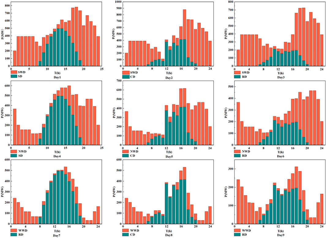
FIGURE 12. Distribution of nine kinds of typical daily wind–PV complementary output.
The fluctuation rule of PV and wind power output under each weather type varies depending on the degree of influence of different meteorological factors, but there is a certain degree of similarity. Since the PV power generates electricity only during the daytime and generally produces more power near noon, wind power normally produces more power at night and reaches an underestimation at noon. As can be seen from the figure, overall, the volatility of the system output after wind and PV power complementation is improved to different degrees in the following nine typical days.
Under different weather conditions, the complementary relationship between PV and wind power systems has obvious differences. On typical “day 1” which combines SD with SWD, and typical “day 6” which combines RD with NWD, the output of the complementary system is significantly improved. The output fluctuation is greatly reduced, the multi-peak characteristic becomes less obvious, and the peak-to-valley difference is also greatly reduced. While the output fluctuation of typical days of most weather types is improved, the effect is not very obvious, such as typical “day 8” which combines RD with WWD.
3.1.5 Analysis of Wind–PV–PHES Complementary System Net Load Characteristics
The random fluctuation of solar and wind energy can have a significant impact on the stability of power systems. Uncontrolled absorption of large amounts of solar and wind energy may lead to drastic power fluctuations in the entire power system over a certain period. Therefore, it is very important to maximize the consumption of PV and wind power without affecting the system, taking into account the operational economics of PV and wind power. An effective way to overcome this problem is to combine the PHES system with intermittent renewable energy sources. The reason is that the PHES system is a relatively mature form of energy storage with low investment costs that can make full use of excess energy and ensure smooth operation of the system.
Solar and wind energy have the characteristics of natural space–time complementarity. The PHES system has the characteristics of energy storage, peak regulation, and frequency regulation, forming a wind–PV–PHES complementary system to make the power system run smoothly. If the PV and wind power generation cannot output at full capacity, the excess solar and wind energy will be available for pumping the stored gravitational potential energy of the lower reservoir. If the PV and wind power generation cannot generate enough power to meet the load requirements, water from the upper reservoir will be used to drive the turbines to generate power. The principle of complementary operation is that the wind–PV complementary system operates at full load according to the day-ahead power forecast, with fluctuations and intervals in output regulated mainly by the PHES system. In other words, while the PHES system is added to the system, the output fluctuations of the complementary operation system will be smoothed out as PV and wind power are fully utilized and the operational efficiency is improved.
To improve the generation efficiency and access capacity of PV and wind power, the energy storage function of the PHES system is used to balance the maximum benefit and minimum output fluctuation of the wind–PV–PHES complementary system. The net load curve of the wind–PV–PHES complementary system after adding the daily load of three typical systems is shown in Figures 13–15.
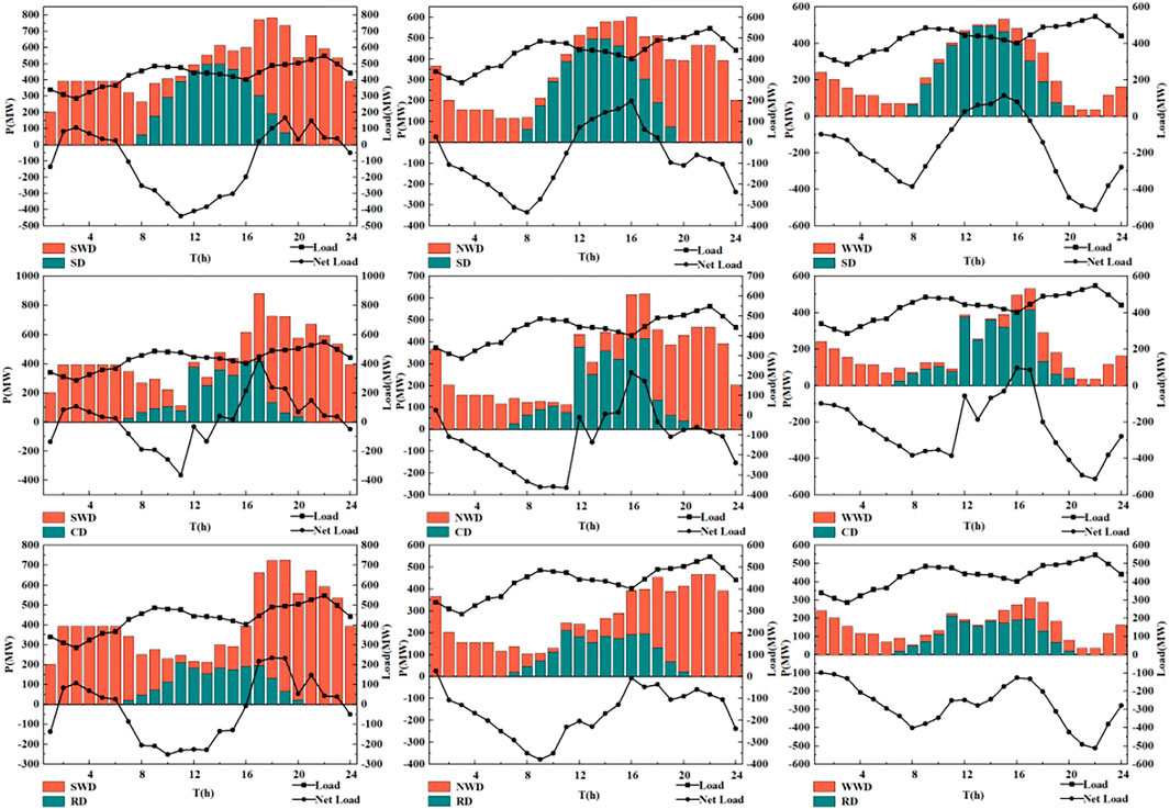
FIGURE 13. Distribution of wind and PV power output and net load curve after adding load one.
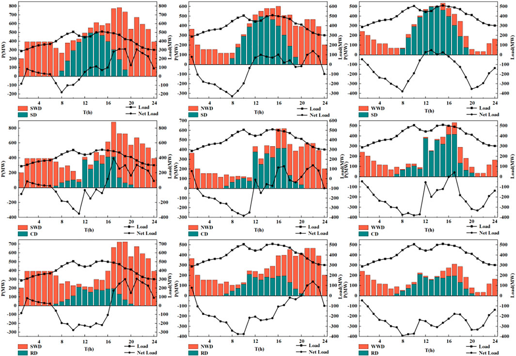
FIGURE 14. Distribution of wind and PV power output and net load curve after adding load two.
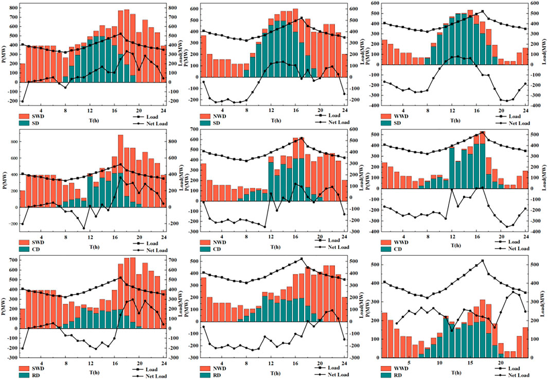
FIGURE 15. Distribution of wind and PV power output and net load curve after adding load three.
As can be seen from the figure, the daily load of all three typical systems fluctuates and is smaller at night and larger during the day. The three typical daily load curves with different peaks and trough periods are representative and can accurately and comprehensively verify the regulation ability of the PHES system. The net load is the difference between the sum of the wind power generation and PV power generation system output and the load of that period, which is the function of the PHES system to adjust the peak and fill the valley of the power system. When the value of a point in the net load curve is less than 0, it means that the wind and PV power output is less than the load value, so the PHES system converts to the turbine condition and releases water to the lower reservoir to make up for the lack of output and ensure the stability of the system load. When the value of a point in the net load curve is greater than 0, it means that the wind and PV power output is greater than the load value, so the PHES system converts to the pump condition and pumps water to the upper reservoir to store energy, reduce the rate of wind and light abandonment, and improve energy utilization.
As shown in Figures 13–15, the maximum net load is 436.1 MW and the minimum value is -513.2 MW, which meets the demand for peak regulation. The PHES system has the functions of quick action, flexibility, fast climbing and unloading, and peak and valley regulation. So they are capable of improving the load fluctuation of the power system and ensuring smooth operation.
3.2 Analysis of the Flow Characteristics of the Pump Turbine to Smooth out the Fluctuation of Wind and Solar Energy Output
3.2.1 Selection of Working Condition Points
As shown in Figure 16, a point from each of the three typical daily net load curves after adding load three is taken as the prototype working condition point for CFD numerical simulation. The output is converted to unit power output P11 by the formula and marked on the P11–n11 curve of the pump turbine model one by one. The P11–n11 curve shows the various main performances of the pump turbine by plotting the iso-efficiency line, the iso-openness line, and the iso-cavitation coefficient line with n11 and P11 as horizontal and vertical coordinates. The main information and the correspondence can be obtained by taking any point of the curve. The three working condition points of the pump turbine model under different openings are as shown in Figure 17, and the conversion formula is as follows.
where
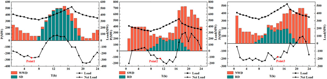
FIGURE 16. Prototype working points in the daily net load curve.
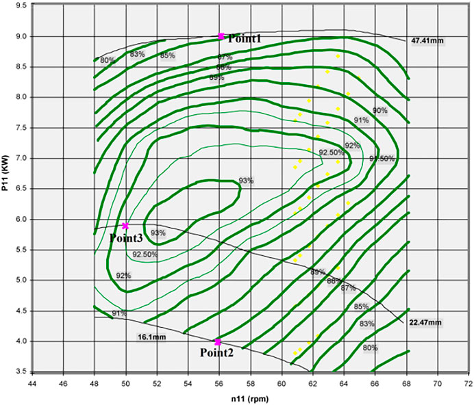
FIGURE 17. Working condition points in the P11–n11 curve.
The relevant parameters of the three working condition points after conversion are listed in Table 3.
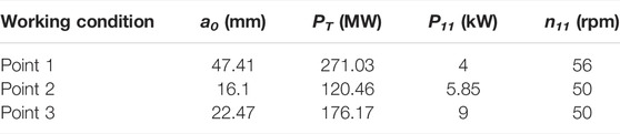
TABLE 3. Relevant parameters of working condition points.
CFD numerical simulations were performed for the aforementioned three working condition points, and the same pressure-based solver settings were used before performing the calculations.
1) Adopting speed inlet.
2) Free outflow (Outflow) is used at the outlet.
3) Dynamic and static interference of runner (Song et al., 2020), using the multi-reference system model (MRF).
4) Coupled calculation of velocity and pressure using the coupled algorithm.
5) Turbulence model using the SST k-ω model and second-order windward discretization.
The parameters required for the three working condition points of the pump turbine before conducting CFD numerical simulations are listed in Table 4.

TABLE 4. Pump turbine pre-treatment parameters.
3.2.2 Flow Characteristics Analysis
3.2.2.1 Water Guide Mechanism
Since both the volute and vane are designed to guide the water flow smoothly into the runner and to form and change the velocity loop of the water flow, the volute and vane are analyzed together. From the pressure distribution diagram of the volute and vane in Figure 18A, it can be seen that the pressure change of the water flow in the volute is basically the same along the centripetal direction under the three working conditions, and only the magnitude of the pressure value is different. The pressure in the circumferential direction is distributed in a band from the outside to the inside, and the pressure gradually decreases along the center of the circle. The pressure size is in the order of the volute, stay vane, and guide vane. Since the volute is segmented, the fluid domain is not smooth at the weld seam, and because the flow rate is larger at the opening of the guide vane a0 = 47.41 mm, there is a slight sudden change in pressure at the weld seam of the volute.
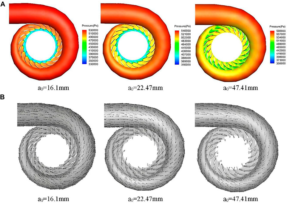
FIGURE 18. Internal flow characteristics of volute and vane. (A) Pressure distribution. (B) Velocity vector.
The pressure variation of the water flow between the walls of the vane is approximately the same for the three operating conditions, with a general tendency to decrease. The pressure at the outer edge of the seat ring, the inlet of the stay vane, and the guide vane is higher. Due to the high-speed flow of water, the water flow in the tip and tail of the vane experiences an impact. The pressure will suddenly reduce, at a0 = 16.1 mm more obvious. At a0 =47.41 mm, the pressure at the back of the vane blade is significantly smaller than that at the waterward side. Due to the dynamic and static interference of the runner, the pressure magnitude changes dramatically in the area from the guide vane to the inlet section of the runner.
From the velocity vector diagrams of the volute and vane in Figure 18B, it can be seen that, on the whole, the water flow in the volute has an equiangular spiral shape in all three operating conditions, which is consistent with the flow characteristics of the water in the volute. The symmetry in the circumferential direction is good, the water flow is uniform and smooth, and the volute can well guide the water flow into the stay vane in an axisymmetric manner.
The velocity distribution of the water flow in the vane is relatively uniform, the flow is smooth, the symmetry along the circumferential direction is good, and there is no vortex. After the water flows out of the guide vane and before entering the runner, it can be observed that the velocity direction of a0 = 16.1, 22.47, and 47.41 mm in the three working conditions, and the angle between the guide vane increases in order, and it is close to normal at a0 = 47.41 mm.
3.2.2.2 Runner
From the pressure distribution diagram of the runner in Figure 19A, it can be seen that the pressure distribution of the runner in the three working conditions is relatively uniform and has a certain similar distribution law. The pressure change in the wall of the runner is distributed in a band, and it is symmetrical and decreases uniformly along the circumferential direction, but the pressure magnitude is different. The pressure from the inlet side to the outlet side of the runner decreases gradually. There are different degrees of negative pressure at the outlet and the lower ring of the runner, and the negative pressure zone at a0 = 22.47 mm is relatively large; therefore, the possibility of cavitation is also larger. Since there are narrow gaps between the tip of the runner blade and the edge of the upper crown and lower ring, high-pressure areas will be generated at these gaps when the runner rotates at high speed, which is also the area where cavitation is likely to occur.
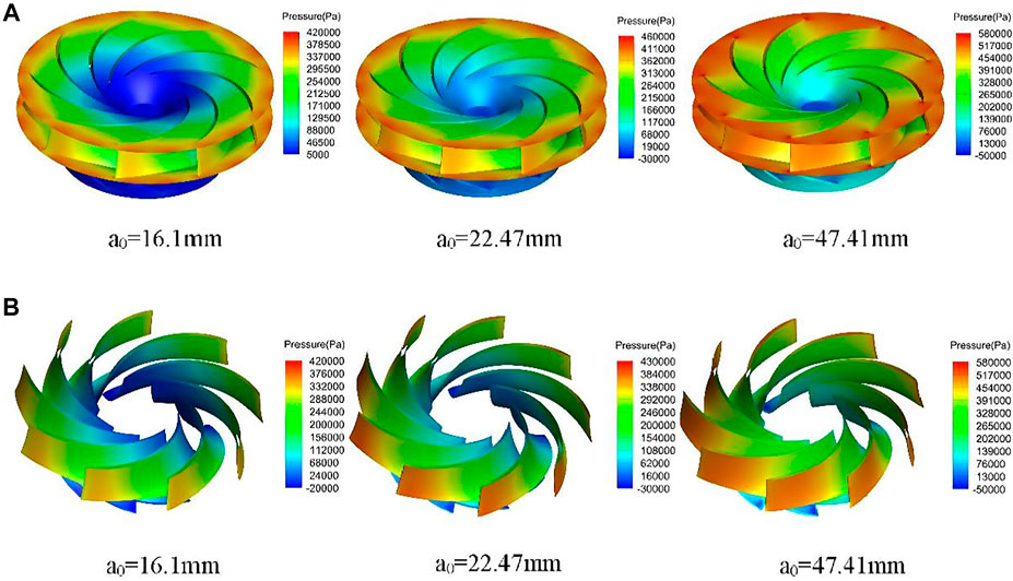
FIGURE 19. Internal flow characteristics of runner. (A) Flow line. (B) Cross-sectional pressure distribution.
The pressure distribution diagram of the runner blades in Figure 19B shows that the pressure distribution law of the blades in the three working conditions is similar. The pressure decreases gradually along the direction of the water flow from the inlet side to the outlet side of the blades, and the pressure distribution of the nine runner blades has symmetry along the circumferential direction, the overall force of the runner is great, and the flow is smooth.
The overall pressure on the waterward side of the blade is greater than that on the backwater side, so the blade forms a certain pressure difference between the waterward side and the backwater side, which drives the runner’s high-speed rotation of the force from this pressure difference. When a0 = 47.41 mm, the pressure difference of the blade between the waterward side and the backwater side is the largest, with different degrees of negative pressure separately. The possibility of these areas occurring in the cavitation is larger, and these areas will cause damage to the runner blade. The following measures can be taken to improve the cavitation performance of the pump turbine.
1) Improving the hydraulic design of the pump turbine.
2) Improving the level of processing technology of the pump turbine and adopting materials with strong corrosion resistance.
3) Taking appropriate operational measures to improve operating conditions.
4) Repairing the pump turbine parts damaged by cavitation.
3.2.2.3 Draft tube
As shown in the flow diagram of the draft tube in Figure 20A, the water flows out of the runner and enters the straight cone section first, and the water flow in the straight cone section under the three working conditions has a more obvious velocity ring volume, forming an eccentric vortex zone. Then, the water enters the elbow pipe, and the flow direction changes here and the flow field changes, forming different degrees of vortex stagnation zone in the elbow section. At a0 = 16.1 mm, the water flow at the elbow pipe is more turbulent, the vortex phenomenon is more obvious, and there is a small backflow. At a0 = 22.47 mm, the water flow at the elbow pipe has small fluctuations. At a0 = 47.41 mm, the water flow at the elbow pipe is relatively smooth, more close to the upper wall, and then enters the diffusion section. As the centrifugal force gradually disappears, the water flows into the horizontal diffusion section through the elbow tube, and the water flows smoothly in the diffusion section under all three conditions.
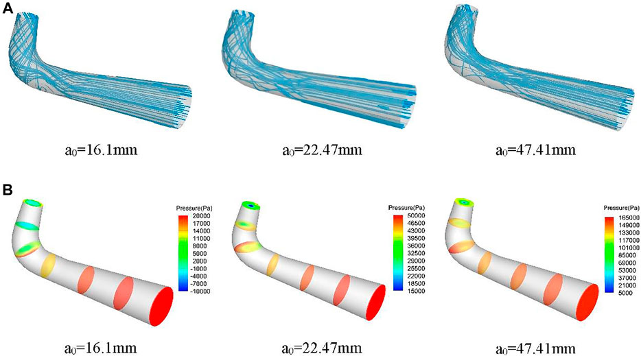
FIGURE 20. Internal flow characteristics of the draft tube: (A), (B).
As shown in the pressure distribution diagram of the draft tube section in Figure 20B, the pressure distribution pattern of the straight cone section under the three working conditions is similar, showing the characteristics of small in the middle and large around. The pressure gradually expands from the center to the circumferential direction. At a0 = 16.1 mm, there are many small pressure mutations at the side wall of the draft tube inlet section. At a0 = 22.47 mm, there is negative pressure at the center of the draft tube inlet section, and there is a certain eccentricity in the pressure distribution at the end of the straight cone section. The pressure in the bent elbow section in the three conditions gradually expands from the center to the circumferential direction. The pressure distribution has different degrees of eccentricity and increases along the direction away from the center of curvature. In the diffusion section of the three conditions, the pressure distribution in each section is more uniform because the water flow gradually tends to be smooth. The pressure distribution in the whole overflow section is basically the same, and the pressure gradually increases in the direction of the draft tube outlet.
4 Conclusion
In this study, the output of wind and PV power systems concerning their volatility was analyzed, CFD numerical simulations of typical working conditions of the pump turbine under wind–PV–PHES complementary systems were conducted, and the following conclusions were drawn.
1) The output of wind and PV power systems varies with the changes in wind speed and solar radiation, respectively, and the output of both fluctuates greatly. The output of the wind power system reaches a trough at noon, and the output at night is larger. The output of the PV power system on SD is approximately normally distributed, and the output reaches a peak at noon. But there are still large fluctuations in the output on RD and CD fluctuates, without obvious rule, and is multi-peaked.
2) Using the natural spatial and temporal complementary characteristics of solar and wind energy, we analyzed the output characteristics of nine typical daily wind–PV complementary systems formed by the arrangement and combination, and found that the output of wind and PV power systems have certain complementary characteristics. But there are still large fluctuations in the output of the complementary systems.
3) In order to improve the power generation efficiency and access capacity of wind and PV power systems, the energy storage function of the PHES system is used to balance the maximum efficiency and minimum output fluctuation of the wind–PV complementary system. After adding three typical system daily loads, 27 net load curves are obtained for the wind–PV–PHES complementary systems. The PHES system pumps and generates electricity to reduce the abandoned wind and light rates and smooth out system fluctuations.
4) There are common points in the laws and characteristics of the internal flow of the pump turbine in different guide vane opening working conditions. At the same time, the different guide vane openings cause the flow in each condition to have its characteristics. CFD technology can well characterize the internal flow characteristics of the pump turbine and provide mechanism analysis for the design and optimization of the pump turbine.
Data Availability Statement
The original contributions presented in the study are included in the article/Supplementary Material; further inquiries can be directed to the corresponding authors.
Author Contributions
YR: methodology, supervision, funding acquisition, and resources. RQ: writing— original draft, formal analysis, and project administration. DW: investigation, data curation, writing—review and editing, and visualization. SH: software model and validation.
Funding
The study was funded by the Henan Province Key R&D and Promotion Project (Science and Technology Research) (Grant No. 212102311054), the Training Program for Young Key Teachers in Colleges and Universities of Henan Province (Grant No. 2019GGJS097), and the Science and Technology Collaborative Innovation Special Project in Zhengzhou city (Research on water system connectivity in realizing rural revitalization strategy of water conservancy) (Grant No. 19).
Conflict of Interest
YR was employed by Yellow River Engineering Consulting Co., Ltd.
The remaining authors declare that the research was conducted in the absence of any commercial or financial relationships that could be construed as a potential conflict of interest.
Publisher’s Note
All claims expressed in this article are solely those of the authors and do not necessarily represent those of their affiliated organizations, or those of the publisher, the editors, and the reviewers. Any product that may be evaluated in this article, or claim that may be made by its manufacturer, is not guaranteed or endorsed by the publisher.
Supplementary Material
The Supplementary Material for this article can be found online at: https://www.frontiersin.org/articles/10.3389/fenrg.2022.914680/full#supplementary-material
Abbreviations
CFD, computational fluid dynamics; PV, photovoltaic; PHES, pumped hydroelectric energy storage; SD, sunny day; CD, cloudy day; RD, rainy day; SWD, strong windy day; WWD, weak windy day; NWD, normal windy day. Symbols: P, output; PT, prototype output; P11, model unit output; Q, flow rate; n, rotational speed; nr, rated rotational speed; n11, unit rotational speed;
References
Abadi, M. H., and El-Saadany, E. F. (2010). Overview of Wind Power Intermittency Impacts on Power Systems [J]. Electr. Power Syst. Res. 80 (6), 627–632. doi:10.1016/j.epsr.2009.10.035
Acuña, L. G., Lake, M., Padilla, R. V., Lim, N. Y., Ponzón, E. G., and Soo Too, Y. C. (2018). Modelling Autonomous Hybrid Photovoltaic-Wind Energy Systems under a New Reliability Approach [J]. Energy Convers. Manag. 172, 357–369. doi:10.1016/j.enconman.2018.07.025
Barra, P. H. A., de Carvalho, W. C., Menezes, T. S., Fernandes, R. A. S., and Coury, D. V. (2021). A Review on Wind Power Smoothing Using High-Power Energy Storage Systems [J]. Renew. Sustain. Energy Rev. 137, 1–18. doi:10.1016/j.rser.2020.110455
Barrio, R., Fernández, J., Blanco, E., Parrondo, J., and Marcos, A. (2011). Performance Characteristics and Internal Flow Patterns in a Reverse-Running Pump-Turbine. Proc. Institution Mech. Eng. Part C J. Mech. Eng. Sci. 226 (3), 695–708. doi:10.1177/0954406211416304
Bogdanovic-Jovanovic, J., Milenkovic, D., Svrkota, D., Bogdanovic, B., and Spasic, Z. (2014). Pumps Used as Turbines Power Recovery, Energy Efficiency, CFD Analysis. Therm. Sci. 18 (3), 1029–1040. doi:10.2298/tsci1403029b
Dianellou, A., Christakopoulos, T., Caralis, G., Kotroni, V., Lagouvardos, K., and Zervos, A. (2021). Is the Large-Scale Development of Wind-PV with Hydro-Pumped Storage Economically Feasible in Greece? [J]. Appl. Sci. 11 (5), 1–21. doi:10.3390/app11052368
Dowds, J., Hines, P., Ryan, T., Buchanan, W., Kirby, E., Apt, J., et al. (2015). A Review of Large-Scale Wind Integration Studies. Renew. Sustain. Energy Rev. 49, 768–794. doi:10.1016/j.rser.2015.04.134
Gao, J., Zheng, Y., Li, J., Zhu, X., and Kan, K. (2018). Optimal Model for Complementary Operation of a Photovoltaic-Wind-Pumped Storage System. Math. Problems Eng. 2018, 1–9. doi:10.1155/2018/5346253
Jurasz, J. (2017). Modeling and Forecasting Energy Flow between National Power Grid and a Solar-Wind-Pumped-Hydroelectricity (PV-WT-PSH) Energy Source. Energy Convers. Manag. 136, 382–394. doi:10.1016/j.enconman.2017.01.032
Koohi-Fayegh, S., and Rosen, M. A. (2020). A Review of Energy Storage Types, Applications and Recent Developments [J]. J. Energy Storage 27, 2–23. doi:10.1016/j.est.2019.101047
Kusakana, K. (2016). Optimal Scheduling for Distributed Hybrid System with Pumped Hydro Storage. Energy Convers. Manag. 111, 253–260. doi:10.1016/j.enconman.2015.12.081
Li, D., Zuo, Z., Wang, H., Liu, S., Wei, X., and Qin, D. (2019). Review of Positive Slopes on Pump Performance Characteristics of Pump-Turbines. Renew. Sustain. Energy Rev. 112, 901–916. doi:10.1016/j.rser.2019.06.036
Olimstad, G., Nielsen, T., and Børresen, B. (2012). Dependency on Runner Geometry for Reversible-Pump Turbine Characteristics in Turbine Mode of Operation [J]. J. Fluids Eng. 134 (12). doi:10.1115/1.4007897
Parastegari, M., Hooshmand, R.-A., Khodabakhshian, A., and Zare, A.-H. (2015). Joint Operation of Wind Farm, Photovoltaic, Pump-Storage and Energy Storage Devices in Energy and Reserve Markets. Int. J. Electr. Power & Energy Syst. 64, 275–284. doi:10.1016/j.ijepes.2014.06.074
Rathore, A., and Patidar, N. P. (2019). Reliability Assessment Using Probabilistic Modelling of Pumped Storage Hydro Plant with PV-Wind Based Standalone Microgrid. Int. J. Electr. Power & Energy Syst. 106, 17–32. doi:10.1016/j.ijepes.2018.09.030
Ren, G., Liu, J., Wan, J., Guo, Y., and Yu, D. (2017). Overview of Wind Power Intermittency: Impacts, Measurements, and Mitigation Solutions. Appl. Energy 204, 47–65. doi:10.1016/j.apenergy.2017.06.098
Sinha, S., and Chandel, S. S. (2015). Review of Recent Trends in Optimization Techniques for Solar Photovoltaic-Wind Based Hybrid Energy Systems. Renew. Sustain. Energy Rev. 50, 755–769. doi:10.1016/j.rser.2015.05.040
Song, H., Zhang, J., Huang, P., Cai, H., Cao, P., and Hu, B. (2020). Analysis of Rotor-Stator Interaction of a Pump-Turbine with Splitter Blades in a Pump Mode [J]. Mathematics 8 (9), 1465. doi:10.3390/math8091465
Tao, R., and Wang, Z. (2021). Comparative Numerical Studies for the Flow Energy Dissipation Features in a Pump-Turbine in Pump Mode and Turbine Mode [J]. J. Energy Storage 41, 1–14. doi:10.1016/j.est.2021.102835
Wang, L., Yin, J., Jiao, L., Wu, D., and Qin, D. (2011). Numerical Investigation on the "S" Characteristics of a Reduced Pump Turbine Model. Sci. China Technol. Sci. 54 (5), 1259–1266. doi:10.1007/s11431-011-4295-2
Waters, S., and Aggidis, G. A. (2015). Over 2000 Years in Review: Revival of the Archimedes Screw from Pump to Turbine. Renew. Sustain. Energy Rev. 51, 497–505. doi:10.1016/j.rser.2015.06.028
Widmer, C., Staubli, T., and Ledergerber, N. (2011). Unstable Characteristics and Rotating Stall in Turbine Brake Operation of Pump-Turbines [J]. J. Fluids Eng. 133 (4). doi:10.1115/1.4003874
Wu, G., Shao, X., Jiang, H., Chen, S., Zhou, Y., and Xu, H (2020). Control Strategy of the Pumped Storage Unit to Deal with the Fluctuation of Wind and Photovoltaic Power in Microgrid [J]. Energies 13 (2), 1–23. doi:10.3390/en13020415
Wu, K., Zhou, H., and Liu, J. (2014). Optimal Capacity Allocation of Large-Scale Wind-PV-Battery Units. Int. J. Photoenergy 2014, 1–13. doi:10.1155/2014/539414
Xu, X., Hu, W., Cao, D., Huang, Q., Chen, C., and Chen, Z. (2020). Optimized Sizing of a Standalone PV-Wind-Hydropower Station with Pumped-Storage Installation Hybrid Energy System. Renew. Energy 147, 1418–1431. doi:10.1016/j.renene.2019.09.099
Xu, Y., Lang, Y., Wen, B., and Yang, X (2019). An Innovative Planning Method for the Optimal Capacity Allocation of a Hybrid Wind–PV–Pumped Storage Power System [J]. Energies 12 (14), 1–14. doi:10.3390/en12142809
Zare Oskouei, M., and Sadeghi Yazdankhah, A. (2015). Scenario-based Stochastic Optimal Operation of Wind, Photovoltaic, Pump-Storage Hybrid System in Frequency- Based Pricing. Energy Convers. Manag. 105, 1105–1114. doi:10.1016/j.enconman.2015.08.062
Zhang, S., and Qi, J. (2011). Small Wind Power in China: Current Status and Future Potentials. Renew. Sustain. Energy Rev. 15 (5), 2457–2460. doi:10.1016/j.rser.2011.02.009
Zhang, X., Dong, X. J., and Li, X. Y. Study of China's Optimal Concentrated Solar Power Development Path to 2050[J]. Front. ENERGY Res., 2021, 9:doi:10.3389/fenrg.2021.724021
Keywords: wind–PV complementary system, output characteristics, CFD numerical simulation, pump turbine, flow characteristics
Citation: Ren Y, Qiao R, Wei D and Hou S (2022) Research on the Internal Flow Characteristics of Pump Turbines for Smoothing the Output Fluctuation of the Wind–Photovoltaic Complementary System. Front. Energy Res. 10:914680. doi: 10.3389/fenrg.2022.914680
Received: 07 April 2022; Accepted: 10 May 2022;
Published: 21 June 2022.
Edited by:
Xiaoshun Zhang, Northeastern University, ChinaReviewed by:
Wenlong Fu, China Three Gorges University, ChinaLefeng Cheng, Guangzhou University, China
Copyright © 2022 Ren, Qiao, Wei and Hou. This is an open-access article distributed under the terms of the Creative Commons Attribution License (CC BY). The use, distribution or reproduction in other forums is permitted, provided the original author(s) and the copyright owner(s) are credited and that the original publication in this journal is cited, in accordance with accepted academic practice. No use, distribution or reproduction is permitted which does not comply with these terms.
*Correspondence: Yan Ren, cmVueWFuQG5jd3UuZWR1LmNu; Daohong Wei, aHNzZ2psQDE2My5jb20=