Dynamic Response Calculation Algorithm for Floating Offshore Wind Turbines Based on a State-Space Method of Transfer Function

The Cummins equation is commonly applied to describe the motion of floating structures. Because of the convolution term, the efficiency of calculation is low and the error accumulation problems in numerical integration calculation are serious. For those reasons, a dynamic response analysis method of floating structures based on a state-space model is proposed. The method uses the state-space method to replace the force-to-motion relationship of the Cummins equation, that is, transfer function, which transforms the problem of calculating the dynamic response into obtaining the output of the state-space model. The method is easy to implement and avoids the problems caused by the presence of the convolution term.

Introduction

With the development of offshore wind power, offshore wind farms extend to deep sea. Considering economy and reliability, the floating offshore wind turbine is a growing trend. In deep-sea areas, the wind, wave, and current conditions are more complex than that of offshore areas, which means that the floating offshore wind turbine should face a hostile environment. To ensure the safety of floating offshore wind turbines, the dynamic response analysis is an important part of the process of design and service stages (Liu et al., 2020).

The dynamic response of floating offshore wind turbines is a complex process, which includes the response induced by wind and waves. To analyze the hydrodynamics of floating offshore wind turbines, the potential theory is usually applied because the viscous effects of large-size floating offshore structures are weak. Under the assumption of a Gaussian wave process, Faltinsen, 2005 used the first-order potential theory to analyze the dynamic response of floating offshore structures, and calculated the dynamic response in the frequency domain. Compared with the time domain method, the frequency domain method has better computational efficiency. However, the limitation of the frequency-domain method, such as energy leakage, periodic hypothesis, and allowing only the stable response calculation, cannot be avoided. To avoid the shortage of the frequency-domain method, Cummins (1962) proposed a time-domain equation (i.e., Cummins equation) to describe the motion of floating structures. The convolution of the retardation function and velocity of floating structures is applied to express the fluid memory effects. Ogilvie (1964) built the relationship between the hydrodynamic parameters and the retardation function, which provided the possibility of using frequency-domain hydrodynamic parameters to solve the time-domain equation. The indirect time-domain method has been widely applied to analyze the dynamic response of floating structures since it was proposed.

However, the convolution item in the Cummins equation is inconvenient for the analysis and design of a motion control system (Fossen, 2002; Perez, 2002). In addition, the convolution item should use the past history of velocity to calculate the radiation force, which leads to low computational efficiency and error accumulation problems (Lu et al., 2019). To overcome the problem, numerous studies have been conducted. Schmiechen (1973) proposed a state-space method to analyze the transient ship maneuvering problem, which introduced a new method to deal with the convolution term. Since then, the state-space method has been widely applied to analyze the dynamic response of floating offshore structures. Taghipour et al., 2008 used the state-space model replacing the convolution term to calculate the dynamic response of floating structures. Chen et al., 2021 used the more efficient state-space model to replace the time-consuming convolution integral in the Cummins equation and analyzed the nonlinear dynamic responses of a point absorber. Wang (2015) applied the state-space replacement method to estimate the response of a floating offshore wind turbine. Zhu et al., 2021 and Chen et al., 2017 adopted the state-space model method to analyze the nonlinear dynamics of float-over deck installation. Guo et al., 2018 used the state-space model corresponding to the retardation function to solve the Cummins equation and applied the method to wave energy conversion analysis.

In this study, a new state-space model method is applied to calculate the dynamic response of floating offshore wind turbines. The method estimates the state-space models corresponding to the transfer function of floating offshore wind turbines, and uses the estimated state-space models to calculate the dynamic response. A spar-type floating offshore wind turbine is applied to investigate the performance of the proposed method. The accuracy and computational efficiency are discussed in the study.

Excitation Impacting Floating Offshore Wind Turbines

Wind Force

The wind force is the main exciting force acting on floating offshore wind turbines, which affects the dynamic response of floating offshore wind turbines. The blade element momentum (BEM) is commonly applied to estimate the aerodynamic loads of the blades of floating offshore wind turbines. Applying the BEM theory, the thrust and torque of the blade-element can be computed using the following manners (Jonkman and Buhl, 2005):

$d{F}_a=\frac{1}{2}{\rho }_a{v}_r^{2}N\left(C_L\sin \phi -C_D\cos \phi \right)c\mathrm{d}r,(1)$

$d{M}_a=\frac{1}{2}{\rho }_a{v}_r^{2}N\left(C_L\cos \phi -C_D\sin \phi \right)cr\mathrm{d}r,(2)$

where ${\rho }_a$ is the density of air, $v_r$ is the relative wind speed, $N$ is the number of element blades, $C_L$ and $C_D$ are the lift and drag coefficients, respectively, $\phi$ is the inflow angel, and $c$ and $r$ are the chord length and radius of the blade element, respectively. According to the formulas, the wind force impacting the blades can be estimated based on the integral operator.

Wave Force

A floating offshore wind turbine is located in the dynamic ocean, which is excited by sea waves. The JONSWAP spectrum is applied to simulate the irregular wave in the actual ocean. The spectrum is expressed using the following formula (Goda, 1999):

$S\left(f\right)=\alpha H_s^2{T}_m^{-4}{f}^{-5}\exp \left[-\frac{5}{4}{\left(T_{m}f\right)}^{-4}\right]{\gamma }^{\exp \left[-{\left(T_{m}f-1\right)}^2/\left(2{\sigma }^2\right)\right]},(3)$

in which

$\begin{array}{l}\alpha =\frac{0.06238}{0.23+0.0336\gamma -0.185\times {\left(1.9+\gamma \right)}^{-1,}}\\ \cdot \left(1.094-0.01915\ln \gamma \right)\end{array}(4)$

where $H_s$ and $T_m$ are the significant wave height and peak period and $\gamma$ and $\sigma$ are the peak enhancement factor and the peak shape factor, respectively.

Based on the JONSWAP spectrum, the irregular wave can be simulated using the following superposition cosine waves:

$\eta \left(t\right)={\displaystyle \sum _{n=1}^Q{A}_n\cos \left(2\pi {\widehat{f}}_{n}t+{\theta }_n\right)},(5)$

where $A_n=\sqrt{2S\left({\widehat{f}}_n\right)\mathrm{\Delta }{f}_n}$ is the wave height of the components, $Q$ is the number of cosine components, ${\widehat{f}}_n$ is the representative frequency, $\mathrm{\Delta }{f}_n$ is the frequency step, and ${\theta }_n$ is the random phase.

Based on the height and frequency of the wave component, the corresponding wave force is obtained by applying the wave force amplitude operator. According to the principle of linear superposition, the total wave force of the irregular wave can be calculated, which will be used to estimate the dynamic response of floating offshore wind turbines.

Dynamic Response Calculation Method

Cummins Equation and the State-Space Model

The dynamic motion behavior of floating structures is commonly described using the Cummins equation under the assumption of linear theory, ideal fluid, small wave excitation, and body motion based on the potential theory. The motion governing the equation of floating offshore wind turbines is expressed as follows:

$\begin{array}{l}\left(\mathbf{M}+{\mathbf{M}}_{\mathbf{a}}\right)\ddot{\mathbf{q}}\left(t\right)+{\displaystyle {\int }_0^t\mathbf{K}\left(t-\tau \right)}\dot{\mathbf{q}}\left(\tau \right)\mathrm{d}\tau +{\mathbf{B}}_a\dot{\mathbf{q}}\left(t\right)+\mathbf{Cq}\left(t\right)\\ ={\mathbf{f}}_{\mathrm{wave}}\left(t\right)+{\mathbf{f}}_{\mathrm{wind}}\left(t\right)+{\mathbf{f}}_{\mathrm{moor}}\left(t\right)\end{array},(6)$

where $\mathbf{M}$ and ${\mathbf{M}}_{\mathbf{a}}$ are the mass and added mass matrices of the floating structure; $\mathbf{K}\left(t\right)$ is the retardation function matrix; ${\mathbf{B}}_{\mathit{a}}$ is the additional linear damping matrix; $\mathbf{C}$ is the restoring matrix; ${\mathbf{f}}_{\mathrm{wave}}\left(t\right)$, ${\mathbf{f}}_{\mathrm{wind}}\left(t\right)$, and ${\mathbf{f}}_{\mathrm{moor}}\left(t\right)$ are the wave, wind, and mooring forces acting on the floating structure; $\mathbf{q}\left(t\right)$, $\stackrel{\cdot }{\mathbf{q}}\left(t\right)$, and $\stackrel{\cdot \cdot }{\mathbf{q}}\left(t\right)$ are the displacement, velocity, and acceleration vector of the floating structure, respectively.

Implementing the Laplace transform to Eq. 6 and ignoring the initial displacement and velocity, the Cummins equation in the Laplace domain can be expressed as follows:

$\begin{array}{l}\left[s^2\left(\mathbf{M}+{\mathbf{M}}_{\mathbf{a}}\right)+s\tilde{\mathbf{K}}\left(s\right)+s{\mathbf{B}}_a+\mathbf{C}\right]\tilde{\mathbf{q}}\left(s\right)\\ ={\tilde{\mathbf{f}}}_{\mathrm{wave}}\left(s\right)+{\tilde{\mathbf{f}}}_{\mathrm{wind}}\left(s\right)+{\tilde{\mathbf{f}}}_{\mathrm{moor}}\left(s\right),\end{array}(7)$

where $\tilde{\mathbf{K}}\left(s\right)$, $\tilde{\mathbf{q}}\left(s\right)$, ${\tilde{\mathbf{f}}}_{\mathrm{wave}}\left(s\right)$, ${\tilde{\mathbf{f}}}_{\mathrm{wind}}\left(s\right)$, and ${\tilde{\mathbf{f}}}_{\mathrm{moor}}\left(s\right)$ are the Laplace transform of $\mathbf{K}\left(t\right)$, $\mathbf{q}\left(t\right)$, ${\mathbf{f}}_{\mathrm{wave}}\left(t\right)$, ${\mathbf{f}}_{\mathrm{wind}}\left(t\right)$, and ${\mathbf{f}}_{\mathrm{moor}}\left(t\right)$, respectively.

Based on Eq. 7, the dynamic response of floating structures in the Laplace domain can be expressed as follows:

$\tilde{\mathbf{q}}\left(s\right)=\mathbf{H}\left(s\right){\tilde{\mathbf{f}}}_{\mathrm{ext}}\left(s\right),(8)$

where $\mathbf{H}\left(s\right)=\frac{1}{s^2\left(\mathbf{M}+\mathbf{Ma}\right)+s\tilde{\mathbf{K}}\left(s\right)+s{\mathbf{B}}_a+\mathbf{C}}$ is the transfer function, and ${\tilde{\mathbf{f}}}_{\mathrm{ext}}\left(s\right)={\tilde{\mathbf{f}}}_{\mathrm{wave}}\left(s\right)+{\tilde{\mathbf{f}}}_{\mathrm{wind}}\left(s\right)+{\tilde{\mathbf{f}}}_{\mathrm{moor}}\left(s\right)$ is the Laplace transform of the total external loading.

Implementing the inverse Laplace transform to Eq. 8, the response of floating structures induced by external loading can be obtained as follows:

$\mathbf{q}\left(t\right)={\displaystyle {\int }_0^t\mathbf{h}\left(t-\tau \right)}{\mathbf{f}}_{\mathrm{ext}}\left(\tau \right)\mathrm{d}\tau ,(9)$

where $\mathbf{h}\left(t\right)$ is the impulse response function and ${\mathbf{f}}_{\mathrm{ext}}\left(t\right)$ is the inverse Laplace transform function of ${\tilde{\mathbf{f}}}_{\mathrm{ext}}\left(s\right)$. Equation 9 shows that the dynamic response of floating structures can be regarded as the output of a system.

For a linear input-output system, the output of the system can be calculated using the convolution operator of the impulse response function and input. Based on Eq. 9, the ith degree displacement response caused by kth degree external loading is calculated using the following convolution operator:

$q_{ik}\left(t\right)={\displaystyle {\int }_0^t{h}_{ik}\left(t-\tau \right)}{f}_{\mathrm{ext, }\mathit{k}}\left(\tau \right)\mathrm{d}\tau ,(10)$

where $h_{ik}\left(t\right)$ is the ith row and the kth column element of the impulse response function $\mathbf{h}\left(t\right)$, $f_{\mathrm{ext, }\mathit{k}}\left(t\right)$ is the kth element of external loading ${\mathbf{f}}_{\mathrm{ext}}\left(t\right)$.

The convolution simplifies the process of calculating the dynamic response of floating structures, but the numerical calculation of Eq. 10 has the sample disadvantages to the Cummins equation. Therefore, Eq. 10 is equivalently converted to the state-space model form as follows:

$\{\begin{array}{c}\stackrel{\cdot }{\mathbf{z}}\left(t\right)=\mathbf{Az}\left(t\right)+\mathbf{B}{f}_{\mathrm{ext, }\mathit{k}}\left(t\right)\\ q_{ik}\left(t\right)=\mathbf{Cz}\left(t\right)+\mathbf{D}{f}_{\mathrm{ext, }\mathit{k}}\left(t\right),\end{array}(11)$

where A, B, C, and D are the matrices describing the state-space model, which is equivalent to $h_{ik}\left(t\right)$.

Decoupling the Transfer Function Based on Discrete Hydrodynamic Parameters

The Cummins equation is converted to the equivalent state-space model, and the matrices of the state-space model are unknown. To calculate the dynamic response of floating structures, the matrices should be estimated first. The different degree motions of floating structures are coupling, which leads to the impulse response functions being unavailable. The impulse response function and transfer function are Laplace or Fourier transform pairs. To obtain the decoupling impulse response function, the transfer function of floating structures should be first decoupled.

Implementing the Fourier transform to the Cummins equation, the Cummins equation in the frequency domain can be expressed as follows:

$\mathbf{Z}\left(\mathrm{j}\omega \right)\tilde{\mathbf{q}}\left(\mathrm{j}\omega \right)={\tilde{\mathbf{f}}}_{\mathrm{ext}}\left(\mathrm{j}\omega \right),(12)$

where $\mathbf{Z}\left(\mathrm{j}\omega \right)=-{\omega }^2\left[\mathbf{M}+\mathbf{A}\left(\omega \right)\right]+\mathrm{j}\omega \left[\mathbf{B}\left(\omega \right)+{\mathbf{B}}_a\right]+\mathbf{C}$ is the impedance function, $\tilde{\mathbf{q}}\left(\mathrm{j}\omega \right)$ and ${\tilde{\mathbf{f}}}_{\mathrm{ext}}\left(\mathrm{j}\omega \right)$ are the Fourier transform of $\mathbf{q}\left(t\right)$ and ${\mathbf{f}}_{\mathrm{ext}}\left(t\right)$, respectively, $\mathbf{A}\left(\omega \right)$ is the frequency-dependent added mass, and $\mathbf{B}\left(\omega \right)$ is the frequency-dependent damping.

The impedance function is related to the hydrodynamic parameters of $\mathbf{A}\left(\omega \right)$ and $\mathbf{B}\left(\omega \right)$. The hydrodynamic parameters are usually calculated using the numerical method, which means that the hydrodynamic parameters are a series of discrete matrices. The discrete impedance function can be expressed as follows:

$\begin{array}{l}{Z}_{ik}\left(\mathrm{j}{\omega }_l\right)=-{\omega }^2\left[M_{ik}+A_{ik}\left({\omega }_l\right)\right]\\ +\mathrm{j}{\omega }_l\left[B_{ik}\left({\omega }_l\right)+B_{a,ik}\right]+C_{ik}\\ i=\mathrm{1,2},\cdots 6;k=\mathrm{1,2},\cdots ,6;l=\mathrm{1,2},\cdots ,N,\end{array}(13)$

where $Z_{ik}\left(\mathrm{j}{\omega }_l\right)$ is the ith row and kth column element of the discrete impedance function, and $N$ is the number of the discrete frequency.

The discrete impedance function can be calculated by Eq. 13. After obtaining the discrete impedance function matrix, the transfer function of floating structures is estimated by applying the reciprocal operator, that is,

$\mathbf{H}\left(\mathrm{j}{\omega }_l\right)={\left[\mathbf{Z}\left(\mathrm{j}{\omega }_l\right)\right]}^{-1}={\left[\begin{array}{cccc}{Z}_{11}\left(\mathrm{j}{\omega }_l\right)& Z_{12}\left(\mathrm{j}{\omega }_l\right)& \cdots & Z_{16}\left(\mathrm{j}{\omega }_l\right)\\ Z_{21}\left(\mathrm{j}{\omega }_l\right)& Z_{22}\left(\mathrm{j}{\omega }_l\right)& \cdots & Z_{26}\left(\mathrm{j}{\omega }_l\right)\\ ⋮& ⋮& \ddots & ⋮\\ Z_{61}\left(\mathrm{j}{\omega }_l\right)& Z_{26}\left(\mathrm{j}{\omega }_l\right)& \cdots & Z_{66}\left(\mathrm{j}{\omega }_l\right)\end{array}\right]}^{-1}.(\mathrm{14a})$

Based on Eqs 13 and 14a, the transfer function of floating structures is decoupled. The decoupled transfer function will be applied to estimate the equivalent state-space model.

Estimation of the State-Space Model

After obtaining the decoupled transfer function of the floating offshore wind turbine, the corresponding impulse response function (IRF) can be computed by using the inverse Fourier transform as follows:

$h_{ik}\left(t\right)=IFFT\left[H_{ik}\left(\mathrm{j}\omega \right)\right],(\mathrm{14b})$

where “IFFT” denotes the inverse fast Fourier transform.

When applying complex exponential decomposition to the IRF of floating offshore wind turbine structures, the IRF can be expressed by a finite number of exponential components as follows (Liu et al., 2020):

$h_{ik}\left(t\right)={\displaystyle \sum _{n=1}^N{\gamma }_{ik,n}{\mathrm{e}}^{{\lambda }_{ik,n}t}},(15)$

where N is the term number, ${\lambda }_{ik,n}$ is the so-called pole, and ${\gamma }_{ik,n}$ is the corresponding residue.

It is obvious that $\gamma {\mathrm{e}}^{\lambda t}$ and $\gamma /\left(s-\lambda \right)$ are a Laplace transform pair. Implementing the Laplace transform to Eq. 15, the transform function can be expressed using the following pole-residue form:

$H_{ik}\left(s\right)={\displaystyle \sum _{n=1}^N\frac{{\gamma }_{ik,n}}{s-{\lambda }_{ik,n}}}.(16)$

Based on the control theory, the transfer function of a system can be expressed with multiple forms, and the different forms are equivalent. For floating structures, the elements of the transfer function correspond to different systems, and the systems can be expressed using a rational fraction. The relative degree of the numerator and denominator is 2 (Lu et al., 2020). In this case, the pole-residue form of the decoupled transfer function can be converted into the rational fraction as follows:

$H_{ik}\left(s\right)=\frac{{\tilde{q}}_{ik}\left(s\right)}{{\tilde{f}}_{\text{ext}}\left(s\right)}=\frac{a_{ik,n}{s}^n+a_{ik,n-1}{s}^{n-1}+\cdots +a_{ik,0}}{s^{n+2}+b_{ik,n+1}{s}^{n+1}+\cdots +b_{ik,0}}.(17)$

Based on the parameters of the rational fraction, the state-space model corresponding to the transfer function can be obtained, which is expressed as follows (Lu et al., 2020):

$\{\begin{array}{c}\stackrel{\cdot }{\mathbf{z}}\left(t\right)=\widehat{\mathbf{A}}\mathbf{z}\left(t\right)+\widehat{\mathbf{B}}{f}_{\mathrm{ext, }\mathit{k}}\left(t\right)\\ q_{ik}\left(t\right)=\widehat{\mathbf{C}}\mathbf{z}\left(t\right),\end{array}(18)$

in which

$\widehat{\mathbf{A}}=\left[\begin{array}{ccccc}0& 1& 0& \cdots & 0\\ 0& 0& 1& \ddots & 0\\ ⋮& ⋮& \ddots & \ddots & ⋮\\ 0& 0& \cdots & 0& 1\\ -b_{ik,0}& -b_{ik,1}& \cdots & -b_{ik,n}& -b_{ik,n+1}\end{array}\right],\widehat{\mathbf{B}}=\left[\begin{array}{c}0\\ 0\\ ⋮\\ 0\\ 1\end{array}\right],\widehat{\mathbf{C}}=\left[\begin{array}{c}{a}_{ik,0}\\ a_{ik,1}\\ ⋮\\ a_{ik,n}\\ 0\end{array}\right],(19)$

where $\widehat{\mathbf{A}}$, $\widehat{\mathbf{B}}$, and $\widehat{\mathbf{C}}$ are the estimated matrices of the state-space model, which are composed of the estimated parameter of the rational fraction.

Dynamic Response Calculation of Floating Offshore Wind Turbines

The governing motion equation of floating offshore wind turbines is converted to a series of state-space models. The problem of dynamic response calculation can be solved by calculating the output of the state-space models. The ith degree of the freedom response of floating offshore wind turbines is calculated using the following formula:

$q_i\left(t\right)={\displaystyle \sum _{k=1}^6{q}_{ik}\left(t\right)}.(20)$

Numerical Study

To investigate the proposed method, a spar-type floating offshore wind turbine is selected to analyze the dynamic response, which is shown as Figure 1. The spar-type floating offshore wind turbine is located in the sea area with a depth of 320 m. The total draft of the floating offshore wind turbine is 120 m. The spar-type floating offshore wind turbine structure comprises a 5 MW wind turbine, tower, and spar-type platform. The length of the tower is 67.6 m and the weight is 249,718 kg. The spar-type platform has a length of 130 m, which contains two cylinders and a connection cone, and a mooring system with three catenary lines is applied to moor the spar-type platform. Detailed information on the floating offshore wind turbine can be referred to in Jonkman (2010).

FIGURE 1

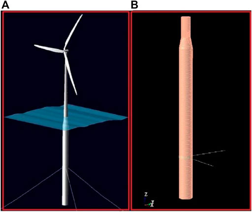
FIGURE 1. Floating offshore wind turbine: (A) total structure model and (B) mesh model.

Hydrodynamic Parameters

To obtain the transfer function of the spar-type floating offshore wind turbine, the hydrodynamic parameters should be first calculated. Considering that the spar-type floating foundation platform is symmetric, the matrices of hydrodynamic parameters have a symmetric property. The symmetric property simplifies the hydrodynamic parameters, and only the upper triangular matrix elements of $\mathbf{A}\left(\omega \right)$ and $\mathbf{B}\left(\omega \right)$ should be considered when calculating the dynamic response of the floating offshore wind turbine. Because of the symmetry, the surge-surge elements of the hydrodynamic parameters are similar to the sway-sway elements, that is, $A_{11}\left(\omega \right)=A_{22}\left(\omega \right)$ and $B_{11}\left(\omega \right)=B_{22}\left(\omega \right)$. Similarly, the roll-roll elements are equal to the pitch-pitch elements, the surge-pitch elements are equal to the pitch-surge elements, and the sway-roll elements are equal to the roll-sway elements.

Based on the aforementioned symmetric property, the non-zero-valued hydrodynamic parameters are calculated using SESAM, which are plotted in Figure 2 and Figure 3, and the frequencies range from 0.01 rad/s–4.985 rad/s with a frequency interval of 0.025 rad/s. The hydrodynamic parameters will be applied to estimate the state-space model of the transfer function.

FIGURE 2

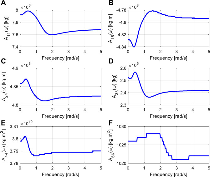
FIGURE 2. Frequency-dependent added mass of floating offshore wind turbines. (A) A11(w); (B) A15 (w); (C) A24(w); (D) A33(w); (E) A44(w) and (F) A66(w).

FIGURE 3

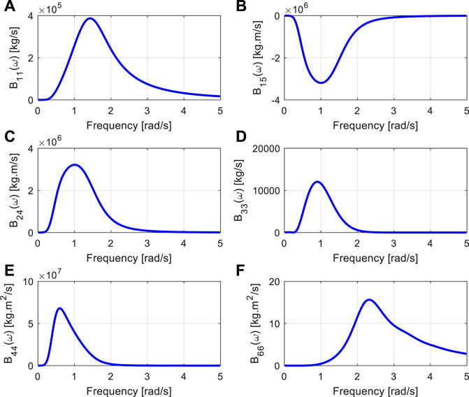
FIGURE 3. Frequency-dependent damping of floating offshore wind turbines. (A) B11(w); (B) B15 (w); (C) B24(w); (D) B33(w); (E) B44(w) and (F) B66(w).

State-Space Model Calculation

Before estimating the state-space model of the transfer function, the transfer function of the spar-type floating offshore wind turbine should be first calculated and decoupled. The viscosity of water is simulated by a linear additional damping matrix. The mooring system restricts the motion of the spar-type floating offshore wind turbine. To simplify the calculation, the mooring force is linearized, which is added to the restoring matrix. In this case, the mass, additional damping, and restoring matrices are listed as follows, which are referred to in Jonkman (2010) and Lu et al. (2020):

$\mathbf{M}=\left[\begin{array}{cccccc}8.151\times {10}^6& 0& 0& 0& -7.329\times {10}^8& 0\\ 0& 8.151\times {10}^6& 0& 7.329\times {10}^8& 0& 0\\ 0& 0& 8.151\times {10}^6& 0& 0& 0\\ 0& 7.329\times {10}^8& 0& 7.541\times {10}^{10}& 0& 0\\ -7.329\times {10}^8& 0& 0& 0& 7.541\times {10}^{10}& 0\\ 0& 0& 0& 0& 0& 8.716\times {10}^7\end{array}\right],(22)$

${\mathbf{B}}_a=\left[\begin{array}{cccccc}1\times {10}^5& 0& 0& 0& 0& 0\\ 0& 1\times {10}^5& 0& 0& 0& 0\\ 0& 0& 1.3\times {10}^5& 0& 0& 0\\ 0& 0& 0& 0& 0& 0\\ 0& 0& 0& 0& 0& 0\\ 0& 0& 0& 0& 0& 1.3\times {10}^7\end{array}\right],(23)$

and

$\mathbf{C}+{\mathbf{C}}_{\mathrm{moor}}=\left[\begin{array}{cccccc}4.118\times {10}^4& 0& 0& 0& -2.821\times {10}^6& 0\\ 0& 4.118\times {10}^4& 0& 2.822\times {10}^6& 0& 0\\ 0& 0& 3.423\times {10}^5& 0& 0& 0\\ 0& 2.816\times {10}^6& 0& 2.538\times {10}^9& 0& 0\\ -2.816\times {10}^6& 0& 0& 0& 2.538\times {10}^9& 0\\ 0& 0& 0& 0& 0& 1.156\times {10}^7\end{array}\right].(24)$

Substituting the matrices and hydrodynamic parameters into Eqs 13, 1, the transfer function of the spar-type floating offshore wind turbine is decoupled, and the discrete transfer function is obtained. Based on the discrete transfer function, the parameters of the rational fractions are estimated by substituting the discrete transfer function into Eq. 18. Only $H_{11}\left(\mathrm{j}\omega \right)$, $H_{15}\left(\mathrm{j}\omega \right)$, $H_{24}\left(\mathrm{j}\omega \right)$, $H_{33}\left(\mathrm{j}\omega \right)$, $H_{44}\left(\mathrm{j}\omega \right)$, and $H_{66}\left(\mathrm{j}\omega \right)$ should be calculated, because they are non-zero values and unique. When implementing the inverse Fourier transform transfer function, the corresponding IRF can be calculated using Eq. 1. After obtaining the estimated IRF, the poles and residues of the IRF are computed by applying complex exponential decomposition. When using Eq. 15 to compute the poles and residues, the decomposition orders of $h_{11}\left(t\right)$, $h_{15}\left(t\right)$, $h_{24}\left(t\right)$, $h_{33}\left(t\right)$, $h_{44}\left(t\right)$, and $h_{66}\left(t\right)$ are set as 6, 4, 4, 4, 2, and 2, respectively. In this case, the comparison of the original and reconstructed IRFs is shown in Figure 4, and the good agreements indicate that the estimated poles and residues are equivalent to the original IRFs.

FIGURE 4

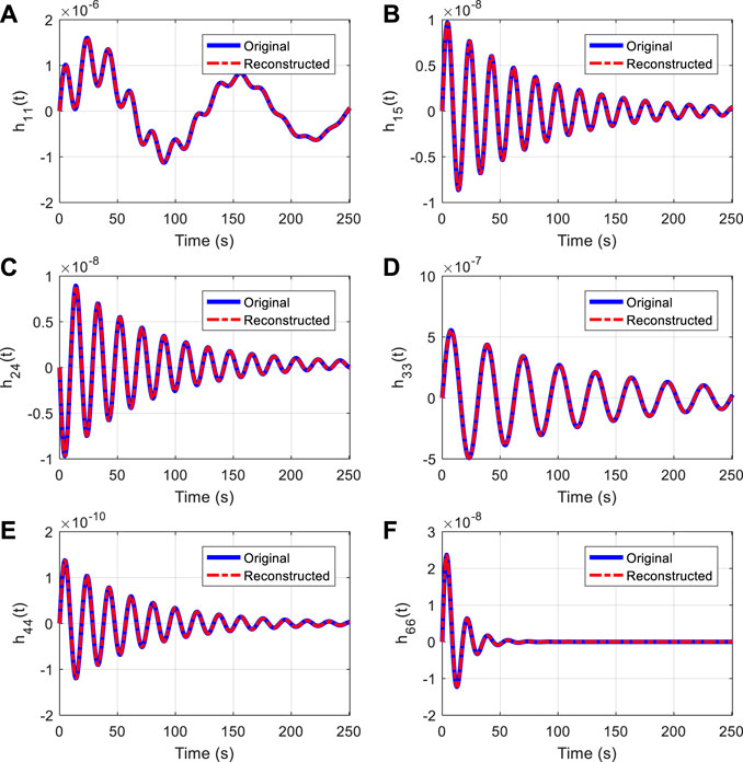
FIGURE 4. Comparison of the original and reconstructed IRF. (A) h11(t); (B) h15 (t); (C) h24(t); (D) h33(t); (E) h44(t) and (F) h66(t).

Based on the poles and residues, the rational fraction of the transfer function can be obtained using Eq. 17. Substituting the frequencies of the hydrodynamic parameter into the estimated transfer function, the real and imaginary parts’ comparison of original and estimated transfer functions are shown in Figure 5 and Figure 6. The good agreement indicates that the estimated transfer function can be applied to calculate the dynamic response of the spar-type floating offshore wind turbine.

FIGURE 5

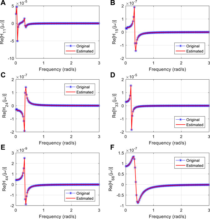
FIGURE 5. Real-part comparison of the original and estimated transfer function. (A) H11(jw); (B) H15 (jw); (C) H24(jw); (D) H33(jw); (E) H44(jw) and (F) H66(jw).

FIGURE 6

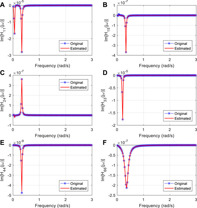
FIGURE 6. Imaginary part comparison of the original and estimated transfer function. Dynamic response calculation of spar-type floating offshore wind turbine. (A) H11(jw); (B) H15 (jw); (C) H24(jw); (D) H33(jw); (E) H44(jw) and (F) H66(jw).

Based on the estimated transfer function, the corresponding state-space models can be constructed using Eqs 18, 19. Then, the problem of the dynamic response calculation for floating offshore wind turbines is converted to calculate the output of a series of state-space model systems, which simplifies the calculation.

The spar-type floating offshore wind turbine is excited by the wind and wave force in service. The wind mainly acts on the blades of the floating offshore wind turbine, and the corresponding wind force was calculated by the BEM theory. When simulating wind force, the wind comprises two forms: homogeneous and turbulent. To show the process of the proposed state-space model method simply, the homogeneous wind is applied to the numerical study. The wind acting on the blades is homogeneous with a speed of 11.4 m/s and a wind shear exponent of 0.143. The rotational speed of the wind turbine is 12.1 rpm. Based on the BEM theory, the equivalent forces impacting the top of the tower are calculated, which are shown in Figure 7.

FIGURE 7

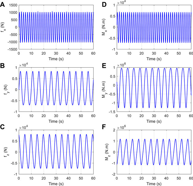
FIGURE 7. Equivalent wind forces. (A) fx(t); (B) fy (t); (C) fz(t); (D) Mx(t); (E) My(t) and (F) Mz(t).

The irregular wave acting on the spar-type floating offshore wind foundation is simulated using the JONSWAP spectrum. The significant wave height is 6 m and the corresponding spectral peak period is 10 s (Jonkman, 2010). Applying the JONSWAP spectrum, the incident wave can be calculated based on Eqs 3–5, which is plotted in Figure 8.

FIGURE 8

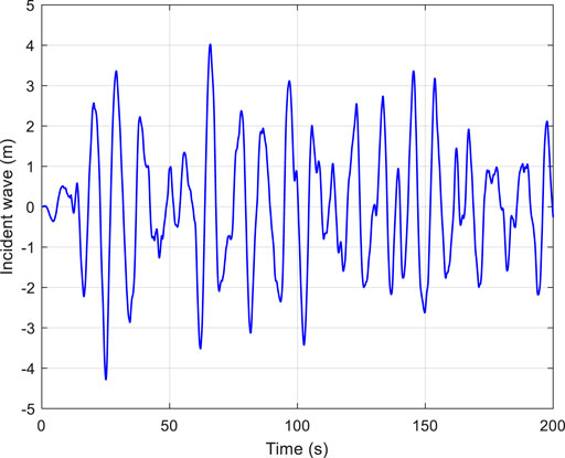
FIGURE 8. Incident wave acting on the spar-type floating offshore wind turbine.

The direction of the incident wave is 0. Based on the JONSWAP spectrum, the frequencies and amplitudes of the wave components are calculated using Eq. 5. The hydrodynamic wave excitation per unit amplitude is computed by hydrodynamic software. Applying the principle of linear superposition, the wave forces induced by the irregular incident wave are obtained. Because of 0° incidence, there are only three DOF wave forces, that is, surge, heave, and pitch, which are shown in Figure 9.

FIGURE 9

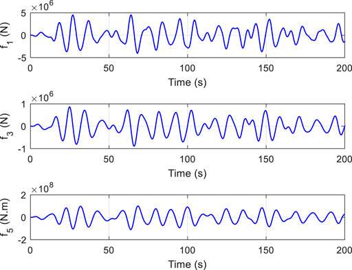
FIGURE 9. Wave force induced by incident waves. (A) f1(t); (B) f3(t) and (C) f5(t).

After obtaining the wave and wind forces acting on the spar-type floating offshore wind turbine, the inputs of the estimated state-space models are obtained. To calculate the dynamic response of the floating offshore wind turbine, the wave and wind forces are substituted into Eqs 18, 20. The outputs of the state-space model are conveniently obtained, that is, the dynamic response. To verify the correctness of the proposed method, the Newmark-β method is also applied to calculate the dynamic response of the spar-type floating offshore wind turbine. The calculated dynamic response comparison of the two methods is plotted in Figure 10, which is in good agreement. The results indicate that the proposed method is able to calculate the dynamic response of the floating offshore wind turbine accurately.

FIGURE 10

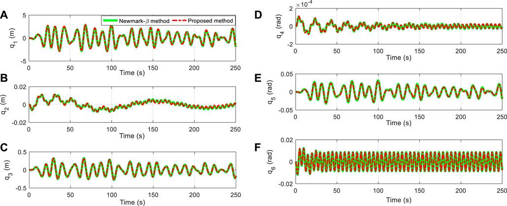
FIGURE 10. Dynamic response comparison of the Newmark-β and proposed methods. (A) q1(t); (B) q2(t); (C) q3(t); (D) q4(t); (E) q5(t) and (F) q6(t).

The proposed method converts the problem of dynamic response calculation to obtaining the output of state-space models, which avoids the convolution calculation and simplifies the process of the dynamic response calculation. The convolution calculation is usually time-consuming and may introduce calculation errors. To investigate the computational efficiency of the proposed method, the elapsed times of the Newmark-β and proposed methods are recorded. The calculation steps change from 500 to 2,500 with an interval of 500. The comparison of elapsed times is shown in Figure 11. The figure shows that the proposed method significantly improves the computational efficiency of the dynamic response of the spar-type floating offshore wind turbine.

FIGURE 11

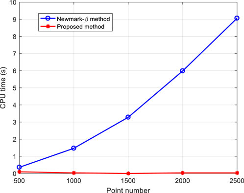
FIGURE 11. Comparison of the computational efficiency.

Conclusions

This study proposes a dynamic response calculation method for floating offshore wind turbines. The method decouples the transfer function and converts the decoupled transfer function to a series of state-space models. The problem of dynamic response calculation is transformed into obtaining the outputs of the estimated state-space models. A spar-type floating offshore wind turbine is applied to investigate the performance of the proposed method. The results show that the proposed method can calculate the dynamic response accurately, and the computational efficiency is considerably higher than that of the Newmark-β method.

Data Availability Statement

The original contributions presented in the study are included in the article/Supplementary Material; further inquiries can be directed to the corresponding author.

Author Contributions

LW and ZS-X proposed the concept of the manuscript. LH-C wrote the first draft of the manuscript and the program codes. LK and FT-H revised the manuscript.

Conflict of Interest

LW and ZS-X were employed by the company Power China Huadong Engineering Corporation Limited.

The remaining authors declare that the research was conducted in the absence of any commercial or financial relationships that could be construed as a potential conflict of interest.

Publisher’s Note

All claims expressed in this article are solely those of the authors and do not necessarily represent those of their affiliated organizations, or those of the publisher, the editors, and the reviewers. Any product that may be evaluated in this article, or claim that may be made by its manufacturer, is not guaranteed or endorsed by the publisher.

Acknowledgments

The authors wish to acknowledge the financial support of the Open Fund of Key Laboratory of Far-shore Wind Power Technology of Zhejiang Province (Grant No. ZOE2021003), the National Natural Science Foundation of China (Grant Nos. 52001126, 52071145, and 51809096), the Natural Science Foundation of Zhejiang province, China (Grant No. LQ21E090010), the Funds for Marine Economic Development of Guangdong, China [Grant Nos. GDNRC (2021)39]. The authors acknowledge the support of OUC.

References

Chen, M., Eatock Taylor, R., and Choo, Y. S. (2017). Investigation of the Complex Dynamics of Float-Over Deck Installation Based on a Coupled Heave-Roll-Pitch Impact Model. Ocean. Eng. 137, 262–275. doi:10.1016/j.oceaneng.2017.04.007

CrossRef Full Text | Google Scholar

Chen, M., Xiao, P., Zhang, Z., Sun, L., and Li, F. (2021). Effects of the End-Stop Mechanism on the Nonlinear Dynamics and Power Generation of a Point Absorber in Regular Waves. Ocean. Eng. 242, 110123. doi:10.1016/j.oceaneng.2021.110123

CrossRef Full Text | Google Scholar

Cummins, W. E. (1962). The Impulse Response Function and Ship Motions[D]. Schiffstechnik 1661, 101–109.

Google Scholar

Faltinsen, O. (2005). Hydrodynamic of High-Speed Marine Vehicles[D]. Cambridge: Cambridge University Press.

Google Scholar

Fossen, T. I. (2002). “Marine Control Systems: Guidance, Navigation and Control of Ships, Rigs and Underwater Vehicles[C],” in Marine Cybernetics. Trondheim, Norway.

Google Scholar

Goda, Y. (1999). A Comparative Review on the Functional Forms of Directional Wave Spectrum. Coast. Eng. J. 41 (1), 1–20. doi:10.1142/s0578563499000024

CrossRef Full Text | Google Scholar

Guo, B., Patton, R. J., Jin, S., and Lan, J. (2018). Numerical and Experimental Studies of Excitation Force Approximation for Wave Energy Conversion. Renew. Energy 125, 877–889. doi:10.1016/j.renene.2018.03.007

CrossRef Full Text | Google Scholar

Jonkman, J. (2010). Definition of the Floating System for Phase IV of OC3 National Renewable Energy Laboratory (NREL). Technical Report NREL/TP-500C47535.

Google Scholar

Jonkman, J. M., and Buhl, J. M. L. (2005). National Renewable Energy Laboratory[C]. FAST Users Guide Gold. 365, 366.

Google Scholar

Liu, F., Gao, S., Liu, D., and Zhou, H. (2020). A Signal Decomposition Method Based on Repeated Extraction of Maximum Energy Component for Offshore Structures. Mar. Struct. 72, 102779. doi:10.1016/j.marstruc.2020.102779

CrossRef Full Text | Google Scholar

Lu, H., Fan, T., Zhou, L., Chen, C., Yu, G., Li, X., et al. (2020). A Rapid Response Calculation Method for Symmetrical Floating Structures Based on State-Space Model Solving in Hybrid Time-Laplace Domain. Ocean. Eng. 203, 107727. doi:10.1016/j.oceaneng.2020.107227

CrossRef Full Text | Google Scholar

Lu, H., Tian, Z., Zhou, L., and Liu, F. (2019). An Improved Time-Domain Response Estimation Method for Floating Structures Based on Rapid Solution of a State-Space Model. Ocean. Eng. 173, 628–642. doi:10.1016/j.oceaneng.2018.12.073

CrossRef Full Text | Google Scholar

Ogilvie, T. (1964). “Recent Progress towards the Understanding and Prediction of Ship Motions[C],” in Sixth Symposium on Naval Hydrodynamics.

Google Scholar

Perez, T. (2002). Ship Motion Control: Course Keeping and Roll Reduction Using Rudder and Fins. Underw. Veh. London, UK: Springer.

Google Scholar

Schmiechen, M. (1973). “On State Space Models and Their Application to Hydrodynamic Systems[C],” in Technical Report, NAUT Report (Department of Naval Architecture, University of Tokyo).

Google Scholar

Taghipour, R., Perez, T., and Moan, T. (2008). Hybrid Frequency-Time Domain Models for Dynamic Response Analysis of Marine Structures. Ocean. Eng. 35, 685–705. doi:10.1016/j.oceaneng.2007.11.002

CrossRef Full Text | Google Scholar

Wang, Y. (2015). Robust Frequency-Domain Identification of Parametric Radiation Force Models for a Floating Wind Turbine. Ocean. Eng. 109, 580–594. doi:10.1016/j.oceaneng.2015.09.049

CrossRef Full Text | Google Scholar

Zhu, L., Zou, M., Chen, M., and Li, L. (2021). Nonlinear Dynamic Analysis of Float-Over Deck Installation for a GBS Platform Based on a Constant Parameter Time Domain Model. Ocean. Eng. 235, 109443. doi:10.1016/j.oceaneng.2021.109443

CrossRef Full Text | Google Scholar