Nonintrusive Load Monitoring Method Based on Color Encoding and Improved Twin Support Vector Machine

In the process of traditional power load identification, the load information of V-I track is missing, the image similarity of V-I track of some power loads is high and the recognition effect is not good, and the training time of recognition model is too long. In view of the abovementioned situation, this study proposes a power load recognition method based on color image coding and the improved twin support vector machine (ITWSVM). First, based on the traditional voltage–current gray trajectory method, the bilinear interpolation technique is used to solve the pixel discontinuity problem effectively. Considering the complementarity of features, the numerical features are embedded into the gray V-I trajectory by constructing three channels, namely, current (R), voltage (G), and phase (B), so the color V-I image with rich electrical features is obtained. Second, the two-dimension Gabor wavelet is used to extract the texture features of the image, and the dimension is reduced by means of local linear embedding (LLE). Finally, the artificial fish swarm algorithm (AFSA) is used to optimize the twin support vector machine (TWSVM), and the ITWSM is used to train the load recognition model, which greatly enhances the model training speed. Experimental results show that the proposed color V-I image coding method and the ITWSVM classification method, compared with the traditional V-I track image construction method and image classification algorithm, improve the accuracy by 6.12% and reduce the model training time by 1071.23 s.

1 Introduction

NILM is the main tool to analyze the electrical behavior of residential users. It can collect, store, and analyze important electrical information through the data acquisition and communication device installed at the user’s power supply entrance. In this way, users can accurately perceive the running state and energy consumption of each electrical equipment (Sun et al., 2017; Guo et al., 2021). Compared with the traditional invasive monitoring device for the analysis of each electrical equipment installation, NILM without further user internal can grasp the electricity situation of all kinds of equipment, on the one hand; reduce the hardware investment, on the other hand; and also remove the existing transformation and maintenance of electrical lines, to a great extent, to protect the user’s privacy (Deng et al., 2020). NILM has a large number of applications in energy efficiency monitoring, fault diagnosis, load modeling, and demand response (Wang and Liu, 2019). In particular, the energy consumption information provided by NILM is of great value for users to understand their own energy consumption structure and guide them to use electricity reasonably, thus realizing energy saving and loss reduction and reducing electricity costs (Zhou et al., 2018; Sun et al., 2020). Therefore, NILM has received extensive attention and strong support from the industry in recent years, and significant progress has been made in related research (Cui et al., 2020; Xiang et al., 2022).

The flow of NILM can be divided into data acquisition, feature extraction, model training, and online recognition. Among them, feature extraction and model training directly affect the accuracy of the algorithm. Feature extraction refers to the use of digital signal processing technology or circuit analysis theory to extract valuable indicators from the collected electrical signals to distinguish different types of electrical equipment. In noninvasive load identification tasks, common load characteristics include voltage and current waveform, current harmonics (Cui et al., 2020), active and reactive power, V-I trajectory (Liu et al., 2021; Xiang et al., 2022), instantaneous power (Li et al., 2021), etc. Among them, V-I trajectory features are characterized by high repeatability and strong stability (Gao et al., 2016; Wu et al., 2020). However, traditional identification methods are prone to misjudge different types of equipment with highly overlapping load characteristics into the same category.

In order to reduce the category and number of misjudgment and realize more efficient model training, new recognition techniques still need to be developed. Scholars at home and abroad have conducted a large number of in-depth studies on V-I trajectory. Liu et al. (2020) extracted the binary V-I trajectory contour to realize the full mining of trajectory shape features. Tu et al. (2018) proposed for the first time to map V-I trajectories into binary grid images, which reduced the computational cost. Zhang et al. (2020) took the binary V-I track image as input to transform the load identification problem into an image classification problem. Due to the outstanding performance of the artificial intelligence algorithm in the field of image classification, the ant colony algorithm is introduced by Du et al. (2016) to extract key features of the weighted pixelated track image, which improves the accuracy of load recognition. Niu et al. (2009) adopted the Fryze power theory to extract reactive current from current, which increased the distinguishing degree of current characteristics. Li et al. (2019) constructed the voltage-reactive current trajectory on the basis of Fryze theory and color-coded the trajectory to integrate other load characteristics. However, its defect was that the trajectory could not reflect the power of the device without combining power characteristics. Wang et al. (2019a) and Chen et al. (2019) used Gram matrix transformation and genetic algorithm, respectively, for power feature fusion, which improves load feature diversity. Although the V-I load identification model and algorithm of trajectory is increasingly mature, there still exists the following problems: trajectory image binary V-I can only transfer trajectory shape information, in principle cannot reflect the power, phase information, such as equipment, and because there are many different kinds of electrical appliances and working principle of the similarity between the different kinds of load V-I trajectory characteristics of overlapping phenomenon. Although the electrical information contained in binary images is more comprehensive, the discontinuity of pixels in V-I image construction will lead to the loss of a lot of useful information, especially the traditional methods cannot fully excavate the advanced features of images. Therefore, the accuracy of load identification still has room for further improvement.

Different from the abovementioned feature extraction and recognition methods, a noninvasive load recognition method based on image coding and the improved twin support vector machine is proposed. This method combines digital features with image features and exploits the outstanding advantages of the improved twin support vector machine in image recognition field to mine the important information contained in electrical signals as much as possible. The main methods are as follows: first, based on the grayscale V-I image, continuous V-I pixels are realized by bilinear interpolation, and three channels, current (R), voltage (G), and phase (B), are constructed by image coding technology to form a continuous color image. Second, two-dimensional Gabor wavelet (Wei et al., 2020) is used to effectively filter the image data to obtain the key texture features of the color V-I image, and LLE dimension reduction is carried out for multiple texture features to reduce the huge amount of calculation caused by high dimension. Third, the parameters of the TWSVM were taken as the position information of artificial fish, and the classification accuracy was taken as the objective function. Then, the optimal location and optimal solution were updated by foraging, clustering, trailing, and random behaviors of ant colony, and the optimal parameters and optimal classification accuracy were obtained at the end of iteration. The algorithm can automatically determine the parameters of the TWSVM in the training process, avoid the blindness of parameter selection, and improve the classification performance of the TWSVM. The characteristics of V-I images are classified by the ITWSVM, the classification results of color V-I images are obtained, and the corresponding electrical equipment classification is completed. Finally, the effectiveness of the proposed method is verified by using the PLAID public data set.

1.1 Continuous V-I Color Image Encoding of Pixel Points

V-I trajectory is a two-dimensional image drawn by a series of voltage and current sampling points in a steady period. For most electrical equipment with different operating principles, the V-I trajectory presents great differences in shape, so various shape parameters (such as area, curvature, number of self-intersection points, and circulation direction) can be extracted from it and used as the basis to distinguish different types of electrical equipment. It is difficult to extract shape parameters, and the parameters after dimensionality reduction cannot fully reflect their original information. Therefore, in the study by Fan et al. (2020), the V-I track is mapped to a binary gray image by using the gridding method while preserving the shape information as much as possible, and the image is used for load identification directly. Compared with the extraction of shape parameters, the process of constructing the binary gray image is simpler. At the same time, the retention of original information is higher, so the accuracy of load identification is further improved.

1.2 Continuous V-I Image Mapping Method

Considering that the V-I image may have pixel discontinuity in the process of mapping, it is not conducive to subsequent training and recognition. Therefore, bilinear interpolation technology is used to improve the traditional mapping method, and the specific process is as follows:

1) A sampling system comprising current clamp, voltage probe, and high-frequency oscilloscope is used to sample the voltage and current waveform of electrical equipment at high frequency, and $M$ is volt-current sampling point $\left(V_m,I_m\right), m=1, 2, \cdots , M$.

2) Given a grid or image resolution of $N\times N$, if all sample points are mapped to the grid, then the size of each cell (pixel point) is

$\{\begin{array}{c}\mathrm{\Delta }\mathit{i}=\frac{{\mathit{i}}_{\mathbf{m}\mathbf{a}\mathbf{x}}-{\mathit{i}}_{\mathbf{m}\mathbf{i}\mathbf{n}}}{\mathit{N}}\\ \mathrm{\Delta }\mathit{v}=\frac{{\mathit{v}}_{\mathbf{m}\mathbf{a}\mathbf{x}}-{\mathit{v}}_{\mathbf{m}\mathbf{i}\mathbf{n}}}{\mathit{N}}\end{array}.(1)$

In Eq. 1, $i_{max}$ and $i_{min}$ are the minimum and maximum values of the current sampling value, respectively. $v_{max}$ and $v_{min}$ are the minimum and maximum voltage sampling values, respectively. $\mathrm{\Delta }i$ and $\mathrm{\Delta }v$ are the dimensions of each cell (pixel point).

3) According to Eq. 2, the distance between two adjacent sampling points after mapping is$D_m\left(m=1, 2, \cdots , M\right)$. If $D_m>1$, it indicates that the distance between two points is greater than the length or width of the cell, indicating discontinuity. Interpolation is needed to complete the interval between two points. For simplicity, bilinear interpolation technology is adopted to realize the filling of discontinuity points, as shown in Eq. 3 and Eq. 4. After filling, the new set of sample points is denoted as $\left(v_j, i_j\right), j=1, 2, \cdots , J$.

${\mathit{D}}_{\mathit{m}}=\sqrt{{\left(\frac{{\mathit{v}}_{\mathit{m}+1}-{\mathit{v}}_{\mathit{m}}}{\mathrm{\Delta }\mathit{v}}\right)}^2+{\left(\frac{{\mathit{i}}_{\mathit{m}+1}-{\mathit{i}}_{\mathit{m}}}{\mathrm{\Delta }\mathit{i}}\right)}^2}.(2)$

${\mathit{v}}_{\mathit{m}+\mathit{k}}^{\prime }={\mathit{v}}_{\mathit{m}}+\frac{{\mathit{v}}_{\mathit{m}+1}-{\mathit{v}}_{\mathit{m}}}{{\mathit{K}}_{\mathit{m}}+1}\mathit{k}\mathit{.}(3)$

${\mathit{i}}_{\mathit{m}+\mathit{k}}^{\prime }={\mathit{i}}_{\mathit{m}}+\frac{{\mathit{i}}_{\mathit{m}+1}-{\mathit{i}}_{\mathit{m}}}{{\mathit{K}}_{\mathit{m}}+1}\mathit{k}\mathit{.}(4)$

In the equations, $K_m=D_m$ is the number of interpolation points to be supplemented between $m$ and $(m +1)$ sampling points. $(v_{m+k}^{\prime },i_{m+k}^{\prime })$ is the $k$ interpolation point of filling, $k=1, 2, \cdots , K_m$.

4) According to Eq. 5, the mapping coordinates of sample points $\left(v_i,i_j\right)$ are calculated as

$\{\begin{array}{c}{\mathit{r}}_{\mathit{j}}=\frac{{\mathit{i}}_{\mathit{j}}-{\mathit{i}}_{\mathbf{m}\mathbf{i}\mathbf{n}}}{\mathrm{\Delta }\mathit{i}}\\ {\mathit{c}}_{\mathit{j}}=\frac{{\mathit{v}}_{\mathit{j}}-{\mathit{v}}_{\mathbf{m}\mathbf{i}\mathbf{n}}}{\mathrm{\Delta }\mathit{v}}\end{array}.(5)$

5) Construct a zero matrix with dimension $N\times N$, and then take out coordinates of all points one by one from the first sample point, and set the elements of row $r_j$ and column $c_j$ in the matrix to one until the last sample point. The obtained matrix is the continuous coordinate matrix of pixel points.

According to the abovementioned method, the gray V-I image of a fluorescent lamp device can be obtained, as shown in Figure 1, with a resolution of 32 × 32. The V-I image obtained by the traditional mapping method has the phenomenon of pixel discontinuity, while the image obtained by the method in this study does not have this problem. The results demonstrate the effectiveness of the abovementioned image construction method.

FIGURE 1

FIGURE 1. Binary V-I trajectory mapping for a fluorescent lamp.

1.3 V-I Color Image Coding Method

According to the analysis in Section 2.1, voltage and current signals of all kinds of electrical equipment are normalized in the process of forming V-I images, and only 0 or one state tables are used for each pixel point. As a result, the V-I image only retains the shape characteristics of voltage–current signals but cannot reflect the numerical differences between devices, especially the numerical characteristics of average current, voltage, power, and phase of devices. For example, the average current of the washing machine and air conditioner is bigger, and the average current of the equipment such as incandescent lamp and computer is lesser. When normalized and mapped, all devices have current values of 0 or 1. Obviously, the gray V-I image has lost a lot of valuable information, so it is difficult to improve the accuracy of load recognition by relying on it alone. Therefore, it is necessary to combine the gray V-I image with the numerical feature to enhance the recognition ability of the algorithm by using the complementarity between the two.

As mentioned earlier, the gray V-I image is a single-channel two-dimensional pixel matrix. Each point in the matrix is 0 or 1, which, respectively, represents whether the point has a V-I trajectory, while the size and direction of the trajectory and other information cannot be reflected. In contrast, for a color image, as shown in Figure 2, it is formed by the superposition of three channels: current (R), voltage (G), and phase (B). Each channel corresponds to a two-dimensional matrix, in which each element can change continuously from 0 to 1. Color images contain more information than gray images. If the numerical information can be embedded into the RGB channel in combination with the shape characteristics of the V-I track, the gray V-I image can be transformed into the corresponding color image. Using this image to classify will undoubtedly improve the recognition accuracy of the whole algorithm.

FIGURE 2

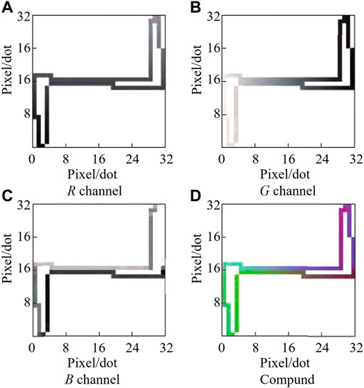
FIGURE 2. Image of each channel of a fluorescent lamp and the synthesized V-I color image.

The core of color image coding lies in the formation of $R$, $G$, and $B$ matrices. The numerical features such as current, voltage (power), and phase are embedded into the corresponding channels to form a color V-I image.

1) Initialize $N \times N$ dimensional $A$, $R$, $G$,and $B$ zero matrices.

2) According to $\left(v_j, i_j\right)$ and Eq. 5, the frequency of occurrence of each coordinate point $A\left(r_j, c_j\right)$ is counted.

3) Construct the current $R$ matrix. Sample points $\left(v_j, i_j\right)$ are taken out one by one, and elements in the $R$ matrix are calculated according to Eq. 6. After the calculation, calculate the average value of each coordinate point according to Eq. 7.

$\mathit{R}\left({\mathit{r}}_{\mathit{j}},{\mathit{c}}_{\mathit{j}}\right)=\mathit{R}\left({\mathit{r}}_{\mathit{j}},{\mathit{c}}_{\mathit{j}}\right)+\mathit{f}\left({\mathit{i}}_{\mathit{j}}\right).(6)$

$\mathit{R}\left({\mathit{r}}_{\mathit{j}},{\mathit{c}}_{\mathit{j}}\right)=\frac{\mathit{R}\left({\mathit{r}}_{\mathit{j}},{\mathit{c}}_{\mathit{j}}\right)}{\mathit{A}\left({\mathit{r}}_{\mathit{j}},{\mathit{c}}_{\mathit{j}}\right)}.(7)$

In Eq. 8, the equation is used to scale the current signal to ensure that elements change continuously from $0-1$. After scaling, the current difference between different devices can be maintained, and the current information of other devices will not be drowned due to the excessive current of some devices.

$\mathit{f}\left({\mathit{i}}_{\mathit{j}}\right)=\frac{1}{\left(1\mathrm{,}{\mathbf{e}}^{2\mathit{ij}}\right)}.(8)$

4) Construct voltage $G$ matrix. Take out sample points $\left(v_j, i_j\right)$ one by one and calculate elements in $G$ matrix according to Eq. 9. After the calculation, calculate the average value of each coordinate point according to Eq. 10.

$\mathit{G}\left({\mathit{r}}_{\mathit{j}},{\mathit{c}}_{\mathit{j}}\right)=\mathit{G}\left({\mathit{r}}_{\mathit{j}},{\mathit{c}}_{\mathit{j}}\right)+\frac{{\mathit{v}}_{\mathit{j}}}{\mathit{V}}.(9)$

$\mathit{G}\left({\mathit{r}}_{\mathit{j}},{\mathit{c}}_{\mathit{j}}\right)=\frac{\mathit{G}\left({\mathit{r}}_{\mathit{j}},{\mathit{c}}_{\mathit{j}}\right)}{\mathit{A}\left({\mathit{r}}_{\mathit{j}},{\mathit{c}}_{\mathit{j}}\right)}.(10)$

Similarly, $V$ maximizes the difference between the maximum and minimum voltages of all devices. If power characteristics are used, $v_j$ and $V$ are replaced by power $p_j$ and $P$, respectively, where $p_j$ is calculated by $p_j=v_j{i}_j$ and $P$ is the maximum power of all devices.

5) Construct the phase $B$ matrix. Sample points $\left(v_j,i_j\right)$ were taken out one by one, and elements in $\text{B}$ matrix were calculated according to Eq. 11 and Eq. 12. After the calculation, calculate the average value of each coordinate point according to Eq. 12.

$\mathit{B}\left({\mathit{r}}_{\mathit{j}},{\mathit{c}}_{\mathit{j}}\right)=\mathit{B}\left({\mathit{r}}_{\mathit{j}},{\mathit{c}}_{\mathit{j}}\right)+\frac{{\mathit{\theta }}_{\mathit{j}}}{2\mathit{\pi }}.(11)$

${\mathit{\theta }}_{\mathit{j}}=\{\begin{array}{c}{\mathit{\delta }}_{\mathit{j}},\\ \mathit{\pi }+{\mathit{\delta }}_{\mathit{j}},\\ 2\mathit{\pi }+{\mathit{\delta }}_{\mathit{j}},\end{array}\begin{array}{c}\mathrm{\Delta }{\mathit{i}}_{\mathit{j}}\ge 0,\mathit{ }\mathrm{\Delta }{\mathit{v}}_{\mathit{j}}\ge 0\\ \mathrm{\Delta }{\mathit{i}}_{\mathit{j}}<0,\mathit{ }\mathrm{\Delta }{\mathit{v}}_{\mathit{j}}\in \forall \\ \mathrm{\Delta }{\mathit{i}}_{\mathit{j}}\ge 0,\mathit{ }\mathrm{\Delta }{\mathit{v}}_{\mathit{j}}<0\end{array}.(12)$

$\mathit{B}\left({\mathit{r}}_{\mathit{j}},{\mathit{c}}_{\mathit{j}}\right)=\frac{\mathit{B}\left({\mathit{r}}_{\mathit{j}},{\mathit{c}}_{\mathit{j}}\right)}{\mathit{A}\left({\mathit{r}}_{\mathit{j}},{\mathit{c}}_{\mathit{j}}\right)}.(13)$

In the equation, ${\theta }_j$ is the phase difference between adjacent points, ${\delta }_j=\text{arc}\tan \left(\frac{\mathrm{\Delta }{v}_j}{\mathrm{\Delta }{i}_j}\right)$, $\mathrm{\Delta }{v}_j=v_{j+1}-v_j$, and $\mathrm{\Delta }{i}_j=i_{j+1}-i_j$, ${\delta }_j\in \left[-\frac{\pi }{2},\frac{\pi }{2}\right]$.

After $R$, $G$, and $B$ matrices are obtained, color V-I images can be obtained by superposing them. According to the abovementioned method, each channel matrix of fluorescent lamp equipment in Figure 1 is constructed, and the results are shown in Figure 2. In Figure 2, the inconsistent light and shade of pixel points in each channel reflect the size and difference of the value (current, voltage, and phase) represented by the point. Because of this difference, the resultant color image can contain more information. To further illustrate this problem, color V-I images of 11 categories of electrical equipment randomly selected from the PLAID dataset are drawn, as shown in Figure 3. Although most of the devices in the figure have different V-I shapes, a few devices are similar, such as air conditioners, electric fans, hair dryers, and incandescent lamps. After careful observation, it can be found that there are obvious differences in color distribution of V-I images in the abovementioned four types of equipment. This is because the average current, phase, and other numerical characteristics of the four types of equipment are inconsistent, resulting in color difference in the corresponding images.

FIGURE 3

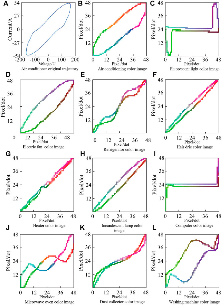
FIGURE 3. Color V-I images of various electrical equipment.

2 Feature Extraction and Dimension Reduction of V-I Color Image

2.1 Two-Dimensional Gabor Wavelet Feature Extraction

In order to extract V-I color image features, this study tries to use two-dimensional Gabor wavelet to extract image texture features and achieve more effective image key texture extraction. Combining with LLE, feature dimension reduction can alleviate feature redundancy and efficiency of high-dimensional feature operation to a certain extent.

As a common tool of image-scale representation and feature analysis, two-dimensional Gabor wavelet can easily realize image scale change. For gray image $z=\left(v_j, i_j\right)$, its filter expression (Li et al., 2019) is as follows:

${\mathit{\phi }}_{\mathit{\alpha },\mathit{\beta }}\left(\mathit{z}\right)=\frac{\Vert {\mathit{k}}_{\mathit{\alpha },\mathit{\beta }}\Vert }{{\mathit{\sigma }}^2}\mathbf{e}\mathbf{x}\mathbf{p}\left(-\frac{{\Vert {\mathit{k}}_{\mathit{\alpha },\mathit{\beta }}\Vert }^2{\Vert \mathit{z}\Vert }^2}{2{\mathit{\sigma }}^2}\right)\cdot \left[\mathbf{e}\mathbf{x}\mathbf{p}\left(\mathit{i}{\mathit{k}}_{\mathit{\alpha },\mathit{\beta }}\right)-\left(-\frac{{\mathit{\sigma }}^2}{2}\right)\right].(14)$

In Eq. 14, $k_{\alpha , \beta }=\left(k_{\beta }\cos {\phi }_{\alpha }, k_{\beta }\sin {\phi }_{\alpha }\right)$ represents the fundamental frequency vector; ${\phi }_{\alpha }$ indicates the direction of $k_{\alpha , \beta }$; $k_{\beta }$ indicates the scale of $k_{\alpha , \beta }$, generally ${\phi }_{\alpha }=\frac{\pi \mu }{8}$, $k_{\beta }=\frac{k_{\mathrm{m}\mathrm{a}\mathrm{x}}}{f^{\beta }}$, $f=\sqrt{2}$, $k_{\mathrm{m}\mathrm{a}\mathrm{x}}=\frac{\pi }{2}$, $\alpha$ and $\beta$ are the direction and scale parameters of two-dimensional Gabor wavelet transform, respectively; and $\sigma$ represents the filtering bandwidth. The main function of $\frac{\Vert {\mathit{k}}_{\mathit{\alpha },\mathit{ \beta }}\Vert }{{\mathit{\sigma }}^2}$ is to compensate the energy attenuation (Wang et al., 2019b) caused by sampling, and $\Vert k_{\alpha , \beta }\Vert$ refers to the two-norm operation. Eq. 15 is divided according to the real and imaginary parts (Moosaei et al., 2021).

$\mathbf{Re}\left({\phi }_{\alpha ,\beta }\left(\mathit{z}\right)\right)=\frac{\Vert {\mathit{k}}_{\mathit{\alpha },\mathit{\beta }}\Vert }{{\mathit{\sigma }}^2}\mathbf{e}\mathbf{x}\mathbf{p}\left(-\frac{{\Vert {\mathit{k}}_{\mathit{\alpha },\mathit{\beta }}\Vert }^2{\Vert \mathit{z}\Vert }^2}{2{\mathit{\sigma }}^2}\right)\cdot \left[\mathbf{cos}\left(\mathit{i}{\mathit{k}}_{\mathit{\alpha },\mathit{\beta }}\right)-\mathbf{e}\mathbf{x}\mathbf{p}\left(-\frac{{\mathit{\sigma }}^2}{2}\right)\right].(15)$

$\mathbf{lm}\left({\phi }_{\alpha ,\beta }\left(\mathit{z}\right)\right)=\frac{\Vert {\mathit{k}}_{\mathit{\alpha },\mathit{\beta }}\Vert }{{\mathit{\sigma }}^2}\mathbf{e}\mathbf{x}\mathbf{p}\left(-\frac{{\Vert {\mathit{k}}_{\mathit{\alpha },\mathit{\beta }}\Vert }^2{\Vert \mathit{z}\Vert }^2}{2{\mathit{\sigma }}^2}\right)\cdot \left[\mathbf{sin}\left(\mathit{i}{\mathit{k}}_{\mathit{\alpha },\mathit{\beta }}\right)\right].(16)$

When two-dimensional Gabor wavelet is carried out, in order to obtain comprehensive image data without loss, it is necessary to set the main parameters $\alpha$, $\beta$, and $\sigma$ of two-dimensional Gabor wavelet reasonably.

2.2 LLE Dimension Reduction

The dimension of the image features obtained by Gabor filtering is high. Considering the problem of feature redundancy and the efficiency of high-dimensional feature operation and storage, it is necessary to effectively reduce the dimension of the image features. The following is a mathematical description of LLE dimension reduction. To achieve dimension reduction for m sample points, suppose that sample $x_i$ can be obtained from its adjacent samples $x_j$, $x_k$, and $x_l$ through linear operation (Gupta and Gupta, 2021).

${\mathit{x}}_{\mathit{i}}={\mathit{\omega }}_{\mathit{ij}}{\mathit{x}}_{\mathit{j}}+{\mathit{\omega }}_{\mathit{ik}}{\mathit{x}}_{\mathit{k}}+{\mathit{\omega }}_{\mathit{il}}{\mathit{x}}_{\mathit{l}}.(17)$

In Eq. 17, ${\omega }_{ij}$, ${\omega }_{ik}$, and ${\omega }_{il}$ are the linear coefficients of sample $x_i$ and its adjacent samples $x_j$, $x_k$, and $x_l$, respectively.

In the actual operation, multiple adjacent samples can be selected for $x_i$. Let the set comprising $k$ neighbor samples of $x_i$ be $Q_i$. In order to maintain the previous linear relationship of sample points after dimensionality reduction, its objective function is Eq. 18 [26].

$\mathbf{m}\mathbf{i}\mathbf{n}{\displaystyle \sum }_{\mathit{i}=1}^{\mathit{m}}{\Vert {\mathit{x}}_{\mathit{i}}-{\displaystyle \sum }_{\mathit{j}\in {\mathit{Q}}_{\mathit{i}}}{\mathit{\omega }}_{\mathit{ij}}{\mathit{x}}_{\mathit{j}}\Vert }^{\mathit{2}}.(18)$

Suppose $C_{jk}={\left(x_i-x_j\right)}^T\left(x_i-x_k\right)$, then

${\mathit{\omega }}_{\mathit{ij}}=\frac{{{\displaystyle \sum }}_{\mathit{k}\in {\mathit{Q}}_{\mathit{i}}}{\mathit{C}}_{\mathit{jk}}^{-1}}{{{\displaystyle \sum }}_{\mathit{l},\mathit{ s}\in {\mathit{Q}}_{\mathit{i}}}{\mathit{C}}_{\mathit{ls}}^{-1}}.(19)$

In Eq. 19, $C_{ls}={\left(x_i-x_l\right)}^T\left(x_i-x_s\right)$.

LLE can keep ${\omega }_{ij}$ unchanged in the dimensionality reduction process, so according to ${\omega }_{ij}$, the sample set after dimensionality reduction can be solved (Li and Ding, 2019).

$min{\displaystyle \sum _{\mathit{i}=1}^m{\Vert {\mathit{z}}_{\mathit{i}}-{\displaystyle \sum _{\mathit{j}\in {\mathit{Q}}_{\mathit{i}}}{\mathit{\omega }}_{\mathit{ij}}{\mathit{z}}_{\mathit{j}}}\Vert }^2}.(20)$

In Eq. 20, ${\mathit{z}}_{\mathit{i}}$ is the value of $x_i$ after dimensionality reduction. By solving the eigenvector corresponding to the eigenvalue of $Z$, the dimensionality reduction set $Z=[z_1, z_2, \cdots ,z_m]$ can be obtained.

3 AFSA Optimize TWSVM

3.1 TWSVM

The TWSVM uses two hyperplanes for classification. The number of samples of the two types is $m_1$ and $m_2$ and the dimension is $n$. The mathematical representation of the two hyperplanes of the TWSVM is Eq. 21 (Shao et al., 2013).

$\mathit{K}\left({\mathit{x}}^{\mathbf{T}},\mathit{ }{\mathit{C}}^{\mathbf{T}}\right){\mathit{\omega }}^{\left(1\right)}+{\mathit{b}}^{\left(1\right)}=0;\mathit{K}\left({\mathit{x}}^{\mathbf{T}},{\mathit{C}}^{\mathbf{T}}\right){\mathit{\omega }}^{\left(2\right)}+{\mathit{b}}^{\left(2\right)}=0.(21)$

In Eq. 21, $K$ is the kernel function, $C=\left[A;B\right]$ represents all training samples, ${\omega }_i\left(i=1, 2\right)$ is the normal vector of the classified hyperplane, and $b_i\left(i=1, 2\right)$ is the bias. Let $A\in R^{m_1\times n}$, $B\in R^{m_2\times n}$, $A={\left(x_1^{\left(1\right)},x_2^{\left(1\right)}, \cdots , x_{m_1}^{\left(1\right)}\right)}^T$, and $B={\left(x_1^{\left(2\right)},x_2^{\left(2\right)},\cdots ,x_{m_1}^{\left(2\right)}\right)}^T$, then the solution of the two hyperplanes can be converted to Eq. 22 and Eq. 23 (Gupta and Gupta, 2021).

TWSVM1:

$\underset{{\mathit{\omega }}^{\left(1\right)},{\mathit{b}}^{\left(1\right)}}{\mathbf{min}}\frac{1}{2}{\left(\mathit{A}{\mathit{\omega }}^{\left(1\right)}+{\mathit{e}}_1{\mathit{b}}^{\left(1\right)}\right)}^{\mathbf{T}}\left(\mathit{A}{\mathit{\omega }}^{\left(1\right)}+{\mathit{e}}_1{\mathit{b}}^{\left(1\right)}\right)+{\mathit{c}}_1{\mathit{e}}_2^{\mathbf{T}}\mathit{\xi }\underset{x\to \infty }{\lim }.$

$\mathbf{s}\mathbf{.t}\mathbf{.}-\left(\mathit{B}{\mathit{\omega }}^{\left(1\right)}+{\mathit{e}}_2{\mathit{b}}^{\left(1\right)}\right)+\mathit{\xi }\ge {\mathit{e}}_2,\mathit{\xi }\ge 0.(22)$

TWSVM2:

$\underset{{\mathit{\omega }}^{\left(2\right)},{\mathit{b}}^{\left(2\right)}}{\mathbf{min}}\frac{1}{2}{\left(\mathit{B}{\mathit{\omega }}^{\left(12\right)}+{\mathit{e}}_2{\mathit{b}}^{\left(2\right)}\right)}^{\mathbf{T}}\left(\mathit{B}{\mathit{\omega }}^{\left(2\right)}+{\mathit{e}}_1{\mathit{b}}^{\left(2\right)}\right)+{\mathit{c}}_2{\mathit{e}}_1^{\mathbf{T}}\mathit{\eta }\mathit{.}$

$\mathbf{s}\mathbf{.t}\mathbf{.}-\left(\mathit{A}{\mathit{\omega }}^{\left(2\right)}+{\mathit{e}}_1{\mathit{b}}^{\left(2\right)}\right)+\mathit{\eta }\ge {\mathit{e}}_1,\mathit{\eta }\ge 0.(23)$

In the equations, $\xi$ and $\eta$ are slack variables, $e_1={\left(1, 1, \cdots , 1\right)}^{\mathbf{T}}\in {\mathbf{R}}^{m_1}$, $e_2={\left(1, 1, \cdots , 1\right)}^{\mathbf{T}}\in {\mathbf{R}}^{m_2}$, and $c_1$ and $c_2$ are the penalty parameters.

The test sample belongs to whichever hyperplane it is near, if $x$ is in the $r$ class, where $r\in \left\{1, 2\right\}$, such as Eq. 24.

$\mathit{K}\left({\mathit{x}}^{\mathbf{T}},{\mathit{C}}^{\mathbf{T}}\right){\mathit{\omega }}^{\left(\mathit{r}\right)}+{\mathit{b}}^{\left(\mathit{r}\right)}=\underset{\mathit{i}=\mathrm{1,2}}{\mathbf{min}}\left|\mathit{K}\left({\mathit{x}}^{\mathbf{T}},{\mathit{C}}^{\mathbf{T}}\right){\mathit{\omega }}^{\mathit{i}}+{\mathit{b}}^{\left(\mathit{r}\right)}\right|.(24)$

3.2 AFSA

The artificial fish swarm algorithm is an optimization algorithm based on swarm intelligence, which is inspired by the behavior of fish. In the AFSA, each AF adjusts its behavior according to its current state and the state of the surrounding environment. During each iteration, the AF updated themselves through four behaviors: foraging, clustering, tailgating, and randomness (Wu et al., 2007).

Suppose $X_i=\left(x_1,x_2, \cdots , x_n \right)$ is the current state of the artificial fish $A{F}_i$, $Y_i=f\left(X_i\right)$ is the fitness function of $X_i$, $Visual$ is the field of vision of the artificial fish, $try\_number$ is the maximum number of foraging attempts, $\delta$ is the crowding factor, $Step$ represents the step length of artificial fish, and $n_f$ indicates the number of artificial fish in the field of view. For the artificial fish $A{F}_i$, a random state $X_j$ in its field of vision can be represented by Eq. 25, where it is a random number between 0 and 1. When the update condition is met, $A{F}_i$ updates its status with Eq. 26.

${\mathit{X}}_{\mathit{j}}={\mathit{X}}_{\mathit{i}}+\mathit{Visual}\cdot \mathbf{R}\mathbf{a}\mathbf{n}\mathbf{d}\left(\right).(25)$

${\mathit{X}}_{\mathit{i}}^{\mathit{t}+1}={\mathit{X}}_{\mathit{i}}^{\mathit{t}}+\frac{{\mathit{X}}_{\mathit{j}}-{\mathit{X}}_{\mathit{i}}^{\mathit{t}}}{\Vert {\mathit{X}}_{\mathit{j}}-{\mathit{X}}_{\mathit{i}}^{\mathit{t}}\Vert }\mathit{Step}\cdot \mathbf{R}\mathbf{a}\mathbf{n}\mathbf{d}\left(\right).(26)$

The four behaviors of artificial fish are described as follows:

1) Foraging behavior: $A{F}_i$ randomly selects a state within its field of vision with $X_j$ if, in the case of the maxima problem, $Y_i<Y_j$ (which is $Y_i>Y_j$ in the case of minima and can be converted between them) moves one step toward $X_j$ according to Eq. 26. Otherwise, the state $X_j$ is randomly selected again to determine whether the requirement $Y_i<Y_j$ is met. If the requirements are still not met after $try\_number$ times of repeated attempts, the random behavior is performed.

2) Swarm behavior: Assuming $X_c$ is the central position in the field of vision, if $Y_c>Y_i$ and $\frac{Y_c}{n_f}>\delta \cdot Y_i$, it indicates that the partner center has more food and is not crowded and then moves one step toward $X_c$ according to Eq. 26; otherwise, foraging behavior is performed.

3) Rear-end behavior: Assume that $X_b$ is the best position found in the field of vision. If $\frac{Y_b}{n_f}>\delta \cdot Y_i$ indicates that $X_b$ has more food and is not crowded, it moves further in the direction of $X_b$ according to Eq. 26; otherwise, foraging behavior is performed.

4) Random behavior: $A{F}_i$ randomly selects a position in its field of vision and then moves one step in that direction, which is a missing behavior of foraging behavior.

These four behaviors switch between each other under different conditions, and the artificial fish will choose the appropriate behavior to find the location of the better solution.

3.3 TWSVM Improved Based on the AFSA

The core idea of the ITWSVM is to find the optimal parameters of the TWSVM through the AFSA. The position $X_i=\left(x_1,x_2, \cdots , x_n\right)$ of artificial fish $A{F}_i$ corresponds to a set of parameters of the TWSVM. The position is a vector whose dimension represents the number of parameters. The objective function of the TWSVM is the classification accuracy of the TWSVM, and the best position found by the AFSA is the best parameter of the TWSVM.

The algorithm steps of the ITWSVM are as follows:

1) Initial settings include artificial fish swarm size $N$, maximum number of iterations $K$, initial position of each artificial fish, step size $Step$, field of vision $Visual$, number of attempts $try\_number$, crowding factor $\delta$, and parameter upper and lower limits of the TWSVM.

2) Taking the position of artificial fish as a parameter, the classification accuracy of the twin support vector machine was calculated, and the classification accuracy was optimized as the objective function. The fitness value of each artificial fish was obtained, and the optimal position of artificial fish in the whole bureau was recorded.

3) Each artificial fish performed swarm and tail chasing behaviors and judged whether the individual had improved. If it is improved, a better behavior is selected; otherwise, the foraging behavior is performed.

4) Perform the action of artificial fish selection and update the position of each artificial fish.

5) Update the status of the globally optimal artificial fish.

6) Judge whether the maximum number of iterations is reached. If so, output the optimal solution and the corresponding parameter combination; otherwise, increase the number of iterations by one and jump to two).

The flow chart of the ITWSVM is shown in Figure 4, through which the process of the algorithm proposed in this study can be seen intuitively.

FIGURE 4

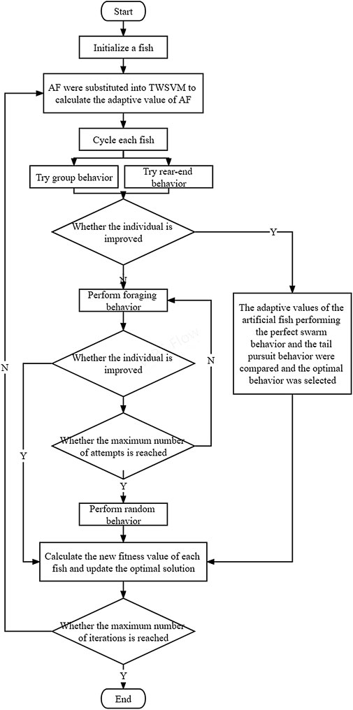
FIGURE 4. Flow chart of the AFSA–TWSVM algorithm.

3.4 Experimental Results and Analysis

In order to prove the effectiveness of the ITWSVM proposed in this study after dimension reduction by LLE, twin support vector machines based on artificial fish swarm algorithm (AFSA–TWSVM) (Li and Ding, 2019) without LLE dimension reduction, twin support vector machines based on particle swarm optimization (PSO–TWSVM) (Shao et al., 2013), twin support vector machines based on fruit fly optimization algorithm (FOA–TWSVM) (Ding et al., 2016), twin support vector machines based on genetic algorithm (GA–TWSVM) (Wang et al., 2013), and twin support vector machines based on glowworm swarm optimization algorithm (GSO–TWSVM) (Ding et al., 2017) were selected as comparative experiments to compare. Considering the rapid development of deep learning in recent years and the excellent performance of the convolutional neural network (CNN) in image classification, this study takes it as a comparative experiment. The V-I color images in section 2 were input into the VGGNet-16 model (Simonyan and Zisserman, 2014) and Fast R-CNN model (Girshick, 2015) for training, and the results were compared.

3.5 The Data Set

The PLAID common data set is used to test the load identification algorithm. The data set comprises voltage and current operation sampling data of 235 electrical equipment in 11 categories of 55 households, with a sampling frequency of 30 kHz and a total sample number of 1074 groups. Considering that the large difference in sample numbers of various electrical equipment in the PLAID data set, it is easy to lead to poor recognition effect of some equipment. For this reason, the synthetic minority over-sampling technique (SMOTE) was used to synthesize and expand a few samples, and the number of expanded samples was 1925. A total of 220 samples (20 samples for each type of equipment) were randomly selected to form the test set, and the remaining 1705 samples were used as the training set.

3.6 Evaluation Functions

For binary classification problems, receiver operating characteristic (ROC) and confusion matrix are important performance indicators for classifier comparison (Zhu and Tang, 2004). Four basic indicators of confusion matrix can be obtained by using the classification results of the test set: true positive (TP), false positive (FP), false negative (FN), and true negative (TN). Based on the abovementioned four basic indicators, the harmonic mean F1 score of accuracy, precision, and recall can be calculated using Eqs. 27,28,29, and30.

$\mathit{Accuracy}=\frac{\mathit{TP}+\mathit{TN}}{\mathit{TP}+\mathit{FP}+\mathit{TN}+\mathit{FN}}\times \mathbf{100}\mathit{\%}\mathit{.}(27)$

$\mathit{Precision}=\frac{\mathit{TP}}{\mathit{TP}+\mathit{FP}}\times \mathbf{100}\mathit{\%}\mathit{.}(28)$

$\mathit{Recall}=\frac{\mathit{TP}}{\mathit{TP}+\mathit{FN}}\times \mathbf{100}\mathit{\%}\mathit{.}(29)$

$\mathit{F}1\mathit{score}=\frac{2\times \mathit{Precision}\times \mathit{Recall}}{\mathit{Precision}+\mathit{Recall}}\times \mathbf{100}\mathit{\%}\mathit{.}(30)$

The ordinate of the ROC curve is true positive rate (TPR), which is the true positive rate, and the ordinate is false positive rate (FPR), which is the false positive rate. TPR and FPR can be obtained by using the basic indicators in the confusion matrix, such as Eq. 31 and Eq. 32.

$\mathit{TPR}=\frac{\mathit{TP}}{\mathit{TP}+\mathit{FN}}\times \mathbf{100}\mathit{\%}\mathit{.}(31)$

$\mathit{FPR}=\frac{\mathit{FP}}{\mathit{FP}+\mathit{TN}}\times \mathbf{100}\mathit{\%}\mathit{.}(32)$

3.7 Analysis

In order to ensure the fairness of algorithm comparison, V-I color track images drawn by the PLAID dataset are used as samples. The maximum number of iterations is 100 because the running period of each intelligent optimization algorithm is different. Each algorithm can only be tested three times, and $\left(c_1, c_2, \sigma \right)$ of the optimal fitness is taken as the optimal parameter of the TWSVM. Table 1 shows the optimal parameter $\left(c_1, c_2, \sigma \right)$ found by different algorithms and the optimal fitness value corresponding to the optimal parameter. Figure 5 shows the curve of LLE + ITWSVM, ITWSVM, PSO-TWSVM, GA-TWSVM, GSO-TWSVM, and FOA-TWSVM parameter optimization process. In the experiment, the optimal parameter $\left(c_1, c_2, \sigma \right)$ obtained by parameter optimization was used as the final TWSVM parameter, and the TWSVM model was established on all the training sets for testing.

TABLE 1

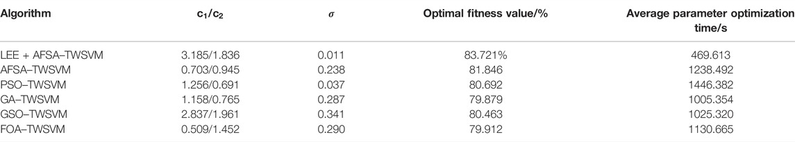
TABLE 1. Comparison of optimization results of different algorithms.

FIGURE 5

FIGURE 5. Optimization process curve of different algorithm parameters.

Figure 6 shows the ROC curves of eleven algorithms. AUC (area under curve) is defined as the area enclosed by the ROC curve and the coordinate axis. AUC provides a digital basis for performance comparison of classification algorithms. To calculate the AUC, only the area under the ROC curve needs to be obtained. Table 2 shows the comparison of the eight algorithms in the four performance indicators of accuracy, F1 score, AUC, and algorithm running time (the running time of TWSVM algorithms includes parameter optimization time) in the test set.

FIGURE 6

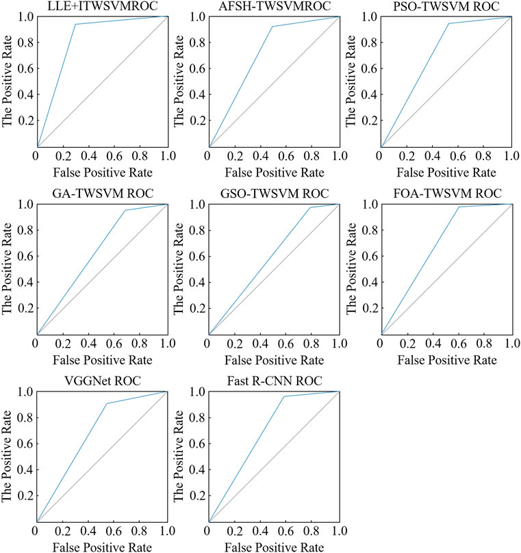
FIGURE 6. ROC curves of different algorithms.

TABLE 2

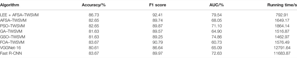
TABLE 2. Comparison of performance indexes of different algorithms.

According to Table 2 and Figure 6, LLE + ITWSVM proposed in this study can find the optimal parameters of the TWSVM faster with fewer iterations. According to Table 2, the proposed LLE + ITWSVM achieves optimal results in the three performance indicators of accuracy, F1 score, and AUC. Meanwhile, the proposed algorithm has the shortest running time and the best real-time performance. It can also be seen from Table 2 that although the Fast R-CNN algorithm achieves a good classification effect, the algorithm is time-consuming because it uses the selective search method to extract candidate regions and there are many redundant operations. All performance indicators of the VGGNET-16 deep convolutional neural network are close to that of the ITWSVM algorithm. In addition, the VGGNET-16 algorithm runs for a long time due to the large amount of computation in the convolutional layer of VGGNET-16 and the larger number of parameters compared with the LLE + ITWSVM algorithm.

Among the six algorithms based on the TWSVM, the proposed LLE + ITWSVM algorithm has the shortest operation time and the best classification performance index. This is mainly due to the dimensionality reduction of V-I color image by LLE, and the calculation of the algorithm after dimensionality reduction is greatly reduced. In addition, the AFSA improved by the TWSVM can jump out of the local optimal solution at a faster speed and find the global optimal parameters suitable for the TWSVM. It solves the problems of TWSVM parameter selection difficulty and parameter optimization algorithm time-consuming in image recognition.

4 Conclusion

Due to the lack of load information of the V-I track in the traditional power load identification process, some power load features overlap and it is difficult to perform equipment identification. The identification model training time is too long. This study presents an intelligent sensing method of power load based on color coding and improved TWSVM. In this method, continuous V-I pixels are realized by bilinear interpolation technology, and the numerical characteristics such as current, voltage, and phase are embedded into the V-I trajectory in the form of different channels so as to form a high-resolution color V-I image. The two-dimensional Gabor wavelet is used to extract image features, and the feature vectors obtained by LLE dimensionality reduction are used for recognition. In addition, an image recognition method based on the AFSA–TWSVM is proposed. This method uses the AFSA algorithm to find the optimal parameters of the TWSVM, which improves the convergence speed and recognition rate of the TWSVM algorithm and overcomes the shortcomings of previous optimization algorithms such as slow convergence speed and easy to fall into local optimal. It provides a new and effective method for the application of TWSVM in V-I color image recognition. Compared with some advanced algorithms, the accuracy of load identification and the speed of model training can be significantly improved by the proposed method, which proves the superiority of the proposed method.

The identification effect of the proposed method for multistate loads needs to be further improved, and a more advanced identification model needs to be built. At the same time, the practical application is still faced with the lack of the domestic data set, high cost of high-frequency sampling, and low universality of the recognition model. Therefore, NILM technology needs further research.

Data Availability Statement

The original contributions presented in the study are included in the article/Supplementary Material; further inquiries can be directed to the corresponding author.

Author Contributions

Conceive, experiment, and write articles.

Conflict of Interest

The authors declare that the research was conducted in the absence of any commercial or financial relationships that could be construed as a potential conflict of interest.

Publisher’s Note

All claims expressed in this article are solely those of the authors and do not necessarily represent those of their affiliated organizations, or those of the publisher, the editors, and the reviewers. Any product that may be evaluated in this article, or claim that may be made by its manufacturer, is not guaranteed or endorsed by the publisher.

Supplementary Material

The Supplementary Material for this article can be found online at: https://www.frontiersin.org/articles/10.3389/fenrg.2022.906458/full#supplementary-material

References

Chen, T., Gao, T., and Zhao, X. M. (2019). Single Sample Description Based on Gabor Fusion. IET image process 13 (14), 2840–2849. doi:10.1049/iet-ipr.2018.6665

CrossRef Full Text | Google Scholar

Cui, L. J., Sun, Y., and Liu, Y. X. (2020). Non-intrusive Load Disaggregation Method Considering Time-Phased State Behavior. Automation Electr. Power Syst. 44 (5), 215–222.

Google Scholar

Deng, X., Zhang, G. Q., and Wei, Q. L. (2020). A Survey on the Non-intrusive Load Monitoring. Acta Autom. Sin. 47 (2), 1–21.

Google Scholar

Ding, S., An, Y., Zhang, X., Wu, F., and Xue, Y. (2017). Wavelet Twin Support Vector Machines Based on Glowworm Swarm Optimization. Neurocomputing 225, 157–163. doi:10.1016/j.neucom.2016.11.026

CrossRef Full Text | Google Scholar

Ding, S., Zhang, X., and Yu, J. (2016). Twin Support Vector Machines Based on Fruit Fly Optimization Algorithm. Int. J. Mach. Learn. Cyber. 7 (2), 193–203. doi:10.1007/s13042-015-0424-8

CrossRef Full Text | Google Scholar

Du, L., He, D., Harley, R. G., and Habetler, T. G. (2016). Electric Load Classification by Binary Voltage-Current Trajectory Mapping. IEEE Trans. Smart Grid 7 (1), 358–365. doi:10.1109/tsg.2015.2442225

CrossRef Full Text | Google Scholar

Fan, L. Y., Hu, C. Z., and Chen, S. Y. (2020). Dimensionality Reduction of Image Feature Based on Geometric Parameter Adaptive LLE Algorithm. Ifs 38 (2), 1569–1577. doi:10.3233/jifs-179520

CrossRef Full Text | Google Scholar

Gao, J., Kara, E. C., and Giri, S. (2016). “A Feasibility Study of Automated Plug-Load Identification from High-Frequency Measurements,” in IEEE Global Conference on Signal ＆ Information Processing Piscataway, New Jersey, USA, 220–224.

Google Scholar

Girshick, R. (2015). “Fast R-CNN,” in IEEE International Conference on Computer Vision. doi:10.1109/iccv.2015.169

CrossRef Full Text | Google Scholar

Guo, H. X., Liu, J. W., and Yang, P. (2021). Review on Key Techniques of Non-intrusive Load Monitoring. Electr. Power Autom. Equip. 41 (1), 135–144.

Google Scholar

Gupta, U., and Gupta, D. (2021). Regularized Based Implicit Lagrangian Twin Extreme Learning Machine in Primal for Pattern Classification. Int. J. Mach. Learn. Cyber. 12 (5), 1311–1342. doi:10.1007/s13042-020-01235-y

CrossRef Full Text | Google Scholar

Li, C., Liang, G. Q., Zhao, G., and Chen, G. (2021). A Demand-Side Load Event Detection Algorithm Based on Wide-Deep Neural Networks and Randomized Sparse Backpropagation. Front. Energy Res. 9, 720831. doi:10.3389/fenrg.2021.720831

CrossRef Full Text | Google Scholar

Li, C. R., Huang, Y. Y., and Xue, Y. (2019). Dependence Structure of Gabor Wavelets Based on Copula for Face Recognition. Expert Syst. Appl. 137, 453–470. doi:10.1016/j.eswa.2019.05.034

CrossRef Full Text | Google Scholar

Li, J. C., and Ding, S. F. (2019). Twin Support Vector Machines Based on Artificial Fish Swarm Algorithm. J. Intelligent Syst. 14 (6), 1121–1126.

Google Scholar

Liu, S., Liu, Y., and Gao, S. (2020). Non-intrusive Load Monitoring Method Based on PCA-ILP Considering Multi-Feature Objective Function. Electr. Power Constr. 41 (8), 1–8.

Google Scholar

Liu, Y., Wang, J. R., Deng, P. X., Sheng, W., and Tan, P. (2021). Non-Intrusive Load Monitoring Based on Unsupervised Optimization Enhanced Neural Network Deep Learning. Front. Energy Res. 9, 718916. doi:10.3389/fenrg.2021.718916

CrossRef Full Text | Google Scholar

Moosaei, H., Ketabchi, S., Razzaghi, M., and Tanveer, M. (2021). Generalized Twin Support Vector Machines. Neural Process Lett. 53 (2), 1545–1564. doi:10.1007/s11063-021-10464-3

CrossRef Full Text | Google Scholar

Niu, H., Quan, C., and Tay, C. J. (2009). Phase Retrieval of Speckle Fringe Pattern with Carriers Using 2D Wavelet Transform. Opt. Lasers Eng. 47 (12), 1334–1339. doi:10.1016/j.optlaseng.2008.10.005

CrossRef Full Text | Google Scholar

Shao, Y., Wang, Z., Chen, W., and Deng, N.-Y. (2013). Least Squares Twin Parametric-Margin Support Vector Machine for Classification. Appl. Intell. 39 (3), 451–464. doi:10.1007/s10489-013-0423-y

CrossRef Full Text | Google Scholar

Simonyan, K., and Zisserman, A. (2014). Very Deep Convolutional Networks for Large-Scale Image Recognition. Available at https://www.arXiv.com/1409-1666.

Google Scholar

Sun, Y., Cui, Can., and Lu, Jun. (2017). Non-intrusive Load Monitoring Method Based on Delta Feature Extraction and Fuzzy Clustering. Automation Electr. Power Syst. 41 (4), 86–91.

Google Scholar

Sun, Y., Li, H. Y., and Liu, Y. X. (2020). Non-intrusive Home-Load Identification Based on Improved Hidden Markov Model. Electr. Power Constr. 41 (4), 73–80.

Google Scholar

Tu, J., Zhou, M., and Song, X. F. (2018). Comparison of Supervised Learning-Based Non-intrusive Load Monitoring Algorithms. Electr. Power Autom. Equip. 38 (12), 128–134.

Google Scholar

Wang, J. S., Ruan, Y. L., and Zheng, B. W. (2019). Face Recognition Method Based on Improved Gabor Wavelet Transform Algorithm. IAENG Int. J. Comput. Sci. 46 (1), 12–24.

Google Scholar

Wang, J., Wong, R. K., and Lee, T. C. M. (2019). Locally Linear Embedding with Additive Noise. Pattern Recognit. Lett. 123, 47–52. doi:10.1016/j.patrec.2019.02.030

CrossRef Full Text | Google Scholar

Wang, P., and Liu, M. (2019). Day-ahead Dispatching Optimization of Active Distribution Network Considering Demand Response. Sci. Technol. Eng. 19 (28), 152–158.

Google Scholar

Wang, Z., Shao, Y., and Wu, T. (2013). A GA-based Model Selection for Smooth Twin Parametric-Margin Support Vector Machine. Pattern Recognit. 46 (8), 2267–2277. doi:10.1016/j.patcog.2013.01.023

CrossRef Full Text | Google Scholar

Wei, H., Hu, C. Z., and Chen, S. Y. (2020). Establishing a Software Defect Prediction Model via Effective Dimension Reduction. Inf. Sci. 477, 399–409.

Google Scholar

Wu, J., Liu, J., and Song, G. T. (2007). Artificial Fish Swarm Algorithm Suitable to Transmission Network Planning. Power Syst. Technol. 31 (8), 63–67.

Google Scholar

Wu, X., Jiao, D., and Gao, Y. C. (2020). Construction of Adaptive Feature Library and Load Identification Based on Decomposition of Non-intrusive Power Consumption Data. Automation Electr. Power Syst. 44 (4), 101–109.

Google Scholar

Xiang, Y. Z., Ding, Y. F., Luo, Q., Wang, P., Li, Q., Liu, H., et al. (2022). Non-Invasive Load Identification Algorithm Based on Color Coding and Feature Fusion of Power and Current. Front. Energy Res. 10, 899669. doi:10.3389/fenrg.2022.899669

CrossRef Full Text | Google Scholar

Zhang, T. Y., Deng, C. Y., and Liu, Y. K. (2020). Non-intrusive Load Identification Algorithm Based on Convolution Neural Network. Power Syst. Tech. 44 (6), 2038–2044.

Google Scholar

Zhou, M., Song, X. F., and Tu, J. (2018). Residential Electricity Consumption Behavior Analysis Based on Non-intrusive Load Monitoring. Power Syst. Technol. 42 (10), 3268–3276.

Google Scholar

Zhu, H., and Tang, X. L. (2004). Classifier Geometrical Characteristic Comparison and its Application in Classifier Selection. PATTERN Recognit. Lett. 26 (6), 829–842.

Google Scholar