Bi-Level Coordinated Planning of Sectionalizing Switches and Tie Lines Considering Operation Mode Adjustment

Distribution utilities can flexibly control distribution networks by allocating the automatic and remotely controlled sectionalizing switches (SSs), which work with tie lines (TLs) to speed up fault management and are alternative devices for distribution operation mode adjustment. Hence, the SSs and the TLs play an important role in distribution networks. In order to improve the reliability of power supply and achieve economic distribution network operation, this paper proposes a bi-level SSs and TLs planning model, which considers distribution operation mode adjustment to optimize the allocation of SSs and TLs. The upper level of the proposed model aims at minimizing the sum of the total investment cost, the customer interruption loss cost, and the line loss cost. The upper level identifies the number and location of the SSs and the TLs. With the planning scheme obtained from the upper level, the lower level of the model adjusts the distribution operation mode to minimize the distribution line loss. In addition, binary particle swarm optimization (BPSO) is used because it has stable convergence and effectively explores the search space. A second-order cone programming (SOCP) is employed to reduce the complexity of the model and improve the solving process by linearizing the reconstruction calculation of the distribution network. Finally, simulation studies were conducted on bus 2 and bus 4 of the RBTS standard test system to assess the feasibility of the proposed model. The stability and effectiveness of the model are verified through various comparisons.

1 Introduction

Power supply plays an increasingly important role in human life and social production, even short-term power interruptions lead to intolerable results. On one hand, it is necessary for power companies to enhance the reliability of power supply and ensure a higher level of customer satisfaction (Fumagalli et al., 2007). On the other hand, distribution operators seek to meet energy demands at the lowest cost when planning and operating their networks (Velasquez et al., 2016). Thus, it is critical to balance the investment, planning, and operation of the distribution networks.

Studies have suggested that approximately 70% of customer outages are caused by the failures of medium-voltage distribution networks (De et al., 2014), and the allocation of sectionalizing switches (SSs) and tie lines (TLs) is regarded as an effective means to improve reliability. With a fault located, the faulted area is isolated using the SSs so that non-faulted areas can be restored as fast as possible. If there is a line without any TLs, SSs just isolate the faulted area and restore the power supply for the upstream load. Otherwise, SSs can also transfer the downstream load with tie switches.

The literature review shows that some heuristic algorithms, such as the simulated annealing algorithm (Billinton and Jonnavithula, 1996), the ant colony algorithm (Falaghi et al., 2008a), the particle swarm optimization algorithm (Bezerra et al., 2014), and the differential evolution algorithm (Ray et al., 2016), have been widely used to obtain the optimal position and number of switches. But these studies only focus on the optimal placement of single types of switches. Considering the cooperation between different types of switches in the fault management process, two novel reliability evaluation algorithms were proposed in Heidari et al. (2016) and Li et al. (2020a) to help determine the optimal locations of SSs and circuit breakers (CBs). The coordinated planning of SSs and fault indicators (FIs) were developed in Falaghi et al. (2008b), Popovic et al. (2017), and Li et al. (2020b) to balance the reliability of power supply and the relevant costs. Taking different users’ economic losses into account, Heidari et al. (2017) and Gholizadeh et al. (2022) presented the new mixed-integer nonlinear programming (MINLP) formulation to determine the allocation of SSs and fuses. A mixed-integer convex formulation and mixed-integer linear programming (MILP) are extended in a study by Heidari et al. (2014) and Lei et al. (2017), respectively, in order to enhance the solution speed and robustness. Meanwhile, the optimal quantity and locations of SSs can be determined by different planning objectives, e.g., minimizing the customer interruption cost, maximizing power supply reliability index, and maximizing restorable loads. Among them, the customer interruption cost is one of the most popular objectives since it links the power supply reliability with the investment economy. As an important part of expansion planning, the placement of TLs has also attracted the research of many scholars. Miranda et al. (1994), Munoz-Delgado et al. (2017), Jooshaki et al. (2019), and Lin et al. (2019) established the expansion planning models for distribution networks, which determined the line corridor and strictly followed the N-1 criterion. In order to minimize the energy loss and energy not supplied (EENS) after an outage, a new method has been adopted to optimize the TLs and the distributed power sources (DGs) simultaneously (Shojaei et al., 2020). However, few studies take the role of TLs in SSs placement into account. Although Sahoo et al. (2012) tried to develop an optimization model for SSs and TLs, it ignored the relationship between SSs and TLs in fault management; the model was only a two-step optimization model.

The typical implementation of SSs and TLs is carried out in a sequential manner, configuring SSs followed by TLs or configuring TL before SSs. With configuring SSs followed by TLs, the role of the SSs have obviously changed following the change in the distribution network, which causes doubtful optimality of SSs. With configuring TLs before SSs, few SSs will be installed after the configuration of TLs if the funds are insufficient, which will fail to effectively improve the reliability and result in a waste of funds. Accordingly, coordinated planning of SSs and TLs that can overcome the above shortcomings and improving the placement of SSs and TLs will be of great importance for a balance between investment and reliability.

Moreover, the configuration of SSs and TLs can provide the equipment basis for the distribution network reconfiguration (e.g., operation mode adjustment). The reconfiguration adjusts the topology of the distribution network during operation by controlling the opening and closing states of SSs and tie switches (Karimi et al., 2021), achieving the optimal operation mode. The optimal objective function of the distribution network is closely related to the objective function of distribution network reconstruction. Hsu et al. (1993), Skoonpong and Sirisumrannukul (2008), and Wang et al. (2021) established distribution, static reconfiguration models, with minimum network losses, balanced load, and maximum reliability as the optimization goals. For the purpose of minimizing the sum of active power, load balance index, and maximum node voltage deviation, Chen et al. (2020) employed the gray target decision-making strategy to select the best problem in the process of solving multi-objective problems. In order to balance the wind energy permeability and voltage stability, Zhong et al. (2020) used the ranking preference technique with the ideal solution similarity to determine the optimal solution on the basis of obtaining the Pareto front.

In order to balance the planning and operation of distribution networks and the balance between the reliability and the economy, the SSs planning can be broadly divided into two sub-problems: optimal allocation of the SSs and the TLs to improve reliability, optimal operation of distribution networks to reduce network losses. When planning different types of content, bi-level models are more effective to obtain a relatively better solution for distribution planning (Sannigrahi et al., 2019). Zhang et al. (2019) and Du et al. (2019) built the bi-level expansion planning methods for active distribution networks by considering the effect of dynamic reconfiguration on the planning of the DGs and the energy storing system (ESS). To solve the operation and energy optimization problems of multi-microgrid power distribution systems, a novel bi-level model was developed (Xu et al., 2021), in which the upper-level model ensured the stability of the voltage while the lower-level model achieved the ultimate goal of minimizing operating costs.

Since bi-level models have become increasingly popular in solving power system problems, their application in the field of SSs and TLs planning with multiple factors needs to be developed. This motivates the authors to develop a bi-level planning model, in which the number and location of SSs and TLs are found in the upper-level planning model, whereas in the lower-level planning model, distribution network reconfiguration is evaluated to find the optimal operation mode. Table 1 compares the proposed planning model with those in the literature. The main contributions of this paper are summarized below.

1) A bi-level planning model considering distribution operation mode adjustment is proposed. This model is compatible with the decision-making process of coordinated planning of SSs and TLs and operation mode adjustment, optimizing the objectives of both parties simultaneously.

2) This paper fully considers the influence of operation mode adjustment and solves the problem of quantifying and modeling the cooperative relationship between SSs and TLs. The model can provide references for the allocation of SSs and TLs, locating SSs and TLs for reliability and economic benefit.

TABLE 1

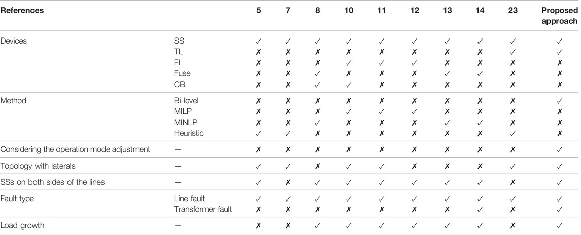
TABLE 1. Comparison of the proposed approach with other literature.

The rest of this paper is organized as follows. Section 2 describes the proposed bi-level model. The solution of bi-level planning model is given in Section 3, and the case studies are presented in Section 4. Finally, this paper is concluded in Section 5.

2 Bi-Level Model

The installation of SSs and TLs plays an important role in reducing EENS and improving the power supply reliability. The adjustment of the operation mode with the minimum line loss as the objective function can effectively reduce the line loss of the distribution network. The specific implementation of these measures is closely related to the distribution network grid and load division. The installation of SSs, the configuration of TLs, and the operation mode adjustment are put into effect step by step in the traditional distribution network planning. So far, little coordination optimization of SSs and TLs has been performed, and operating mode adjustments have rarely been considered along with SSs optimization. However, these three measures can be implemented together to achieve better economic benefits. Although the installation of SSs and TLs will increase equipment costs, it can decrease the cost of customer interruption loss by reducing the EENS. The adjustment of the operation mode with minimum line loss as the objective function will affect both the line loss cost and the investment income of installed SSs. Therefore, this paper proposes a bi-level programming model. At the upper level, a coordinated planning scheme for SSs and TLs is obtained by optimizing the installation quantity and location of SSs and TLs. At the lower level, the line losses of distribution are minimized by shifting the operation mode. Then, the upper level receives the adjusted distribution network topology from the lower level and calculates the objective function. Without TLs, the operation mode adjustment cannot be carried out.

2.1 Upper-Level Model

2.1.1 Objective Function at Upper Level

As mentioned earlier, the upper level is designed to model the SSs and TLs planning problems. As shown in Eq. 1, the objective function consists of three main terms: 1) total investment costs, 2) customer interruption loss cost, and 3) line loss cost.

$UOF=C^{ASS}+C^{INT}+C^{LL}(1)$

The first term models the purchase cost of SSs and TLs from equipment suppliers, installation cost, and operation and maintenance cost. Among them, the first two are one-off costs as shown in Eq. 2, while the operation and maintenance cost is a non-one-off costs that is adopted (Wang et al., 2021). Therefore, interest and inflation rates are included to calculate the present value of SSs operation and maintenance costs because the life cycle of SSs can last several years. The present value of operation and maintenance costs needs to be incorporated into the objective function, which is shown in Eq. 3. The one-off cost and non-one-off cost of SSs and TLs are given in Eq. 4. The one-off cost is determined by the quantity of equipment. For detailed parameter and variable definitions, please refer to the nomenclature.

$\begin{array}{l}OC={\displaystyle \sum _{fn=1}^{N^{fn}}{\displaystyle \sum _{ij\in {\mathrm{\Phi }}_l}(P{C}_{ss}+I{C}_{ss})}}\times (E{S}_{fn,ij,i}+E{S}_{fn,ij,j})\\ +{\displaystyle \sum _{tl=1}^{N^{tl}}(P{C}_{TL}+I{C}_{TL})\times E{T}_{tl}\times L{H}_{tl}}\end{array}(2)$

$\begin{array}{l}NOC={\displaystyle \sum _{lp=1}^{N^{lp}}{\displaystyle \sum _{fn=1}^{N^{fn}}{\displaystyle \sum _{ij\in {\mathrm{\Phi }}_l}\frac{1}{{(1+\mu )}^{lp}}}}\times \delta P{C}_{ss}\times (E{S}_{fn,ij,i}+E{S}_{fn,ij,j})}\\ +{\displaystyle \sum _{lp=1}^{N^{lp}}{\displaystyle \sum _{tl=1}^{N^{tl}}\frac{1}{{(1+\mu )}^{lp}}\times \delta P{C}_{TL}\times E{T}_{tl}}\times L{H}_{tl}}\end{array}(3)$

$C^{ASS}=OC+NOC(4)$

In Eqs 2, 3, $N^{fn}$, $N^{fn}$ and $N^{lp}$ represent the number of feeders, the number of alternative TLs, and the service life of the equipment, respectively. ${\Phi }_l$ is the collection of branch lines in the feeder. $P{C}_{ss}$ and $I{C}_{ss}$ indicate the purchase unit price and installation unit price of the SSs, respectively. $E{S}_{fn,ij,i}$ and $E{S}_{fn,ij,j}$ are the binary variables indicating whether to install SSs, as shown in Eq. 5. $E{T}_{fn,ij}$ is a binary variable indicating whether to install the TL, where $L{H}_{fn,ij}$ is the length of the corresponding TL. Since there are many variables in the Equations, for ease of understanding, Figure 1 is introduced in this paper. As seen from Figure 1, lowercase letters and combined lowercase letters are used to denote nodes (e.g., $h$ is a bus node, $i,j,k$ are branch nodes, and $o,p,q$ are load nodes.) and branches (e.g., $ij$ represents non-load branch from node $i$ to node $j$ and $io$ shows load branch from node $i$ to node $o$.) in the network. If there is a SS installed at $i$ terminal of branch $ij$ of feeder $fn$, $E{S}_{fn,ij,i}=1$, otherwise $E{S}_{fn,ij,i}=0$. Similarly, whether to install a TL is shown in Eq. 6.

$E{S}_{fr,ij,i},E{S}_{fr,ij,j}=\{\begin{array}{l}1\mathrm{SS}\mathrm{present}\mathrm{at}i\mathrm{terminal}\mathrm{and}j\mathrm{terminal}\\ \text{of }\mathrm{branch}ij\mathrm{of}\mathrm{feeder}fr\mathrm{respectively}\text{, }\\ 0\mathrm{otherwise}.\end{array}(5)$

$E{T}_{tl}=\{\begin{array}{l}1\mathrm{TL}\mathrm{is}\mathrm{installed}\mathrm{at}tl\text{,}\\ 0\mathrm{otherwise}\text{.}\end{array}(6)$

FIGURE 1

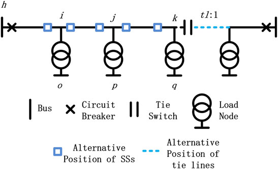
FIGURE 1. An example of a distribution network.

The second term of Eq. 1, customer interruption cost, is defined by Eq. 7 where the average failure rate of network components, the customer outage duration, the customer outage unit cost, and the load increment ratio are taken into account. The average failure rate of the network components and the customer outage duration is determined by the type of failure. Two types of faults are considered in this study, namely line fault and transformer fault. In this paper, $T{R}_{pn,ft,tf}$ indicates the duration of the fault at $pn-th$ load node when the $ft-th$ failure type fault occurs at the $tf-th$ location. $P{R}_{fn,pn}$ represents the average load of the $pn-th$ load node of the $fn-th$ feeder, which is not affected by the fault locations or fault types. $C{C}_{fn,pn}$ adopts the average electricity price conversion multiple methods and is calculated (Liao et al., 2018), which is shown in Eq. 8.

$\begin{array}{l}{C}^{INT}={\displaystyle \sum _{lp=1}^{N^{lp}}{\displaystyle \sum _{fn=1}^{N^{fn}}{\displaystyle \sum _{pn=1}^{N^{pn}}{\displaystyle \sum _{ft=1}^{N^{ft}}{\displaystyle \sum _{tf=1}^{N^{tf}}\frac{1}{{(1+\mu )}^{lp}}\times {\beta }_{tf}}}}}}\\ \times C{C}_{fn,pn}\times T{R}_{pn,ft,tf}\times P{R}_{fn,pn}\times {(1+\gamma )}^{lp-1}\end{array}(7)$

$C{C}_{fn,pn}=U{C}_{fn,pn}\times \chi (8)$

where $\beta$ represents the average failure rate of electric equipment, $\mu$ is the inflation rate, and $\gamma$ indicates the annual load increment rate. $U{C}_{fn,pn}$ and $\chi$ are the unit price of customer interruption cost and the price conversion coefficient, respectively.

The third term of Eq. 1 represents the line loss of the distribution network, which is related to the open-loop location of the distribution network during operation. In this paper, the reconstruction of the distribution network is developed in the lower-level model, and Eq. 9 is used to calculate the line loss.

$C^{LL}={\displaystyle \sum _{lp=1}^{N^{lp}}{\displaystyle \sum _{fn=1}^{N^{fn}}\frac{{(1+\gamma )}^{lp-1}}{{(1+\mu )}^{lp}}\times LO{F}_{fn}}}(9)$

2.1.2 Constraints at Upper Level

There is a cap on the total annual investment cost of the power company. The purpose of distribution network planning is not only for economic optimization but also to meet certain reliability standards to ensure reliable electricity consumption. Therefore, the constraints for the current study are defined by Eqs 10, 11, restraining the maximum available one-off cost and minimum limit reliability, respectively.

$OC\le O{C}^{max}(10)$

$R_{fn}\ge R_{limit-fn},fn\in {\mathrm{\Phi }}_{fn}(11)$

2.2 Lower-Level Model

2.2.1 Objective Function at Lower Level

An optimal distribution network operation is determined at the lower level by minimizing the active power loss, as represented in Eq. 12.

$LOF={\displaystyle \sum _{\left(ij\right)\in {\mathrm{\Phi }}_l}{R}_{ij}\frac{P_{ij}^2+Q_{ij}^2}{V_i^2}}(12)$

If expressed in the form of branch current $I_{ij}$, the objective function at lower level is Eq. 13. Eq. 14 indicates the relationship between $I_{ij}$ and $P_{ij}$, $Q_{ij}$, $V_i$.

$LOF={\displaystyle \sum _{\left(ij\right)\in {\mathrm{\Phi }}_l}{R}_{ij}{I}_{ij}^2}(13)$

$I_{ij}^2=\frac{P_{ij}^2+Q_{ij}^2}{V_i^2}(14)$

2.2.2 Constraints at Lower Level

1) Radial Topology Constraints

In order to reduce the difficulty of relay protection and limit the short-circuit current, the distribution network generally operates radially, which means there is no loop in the network. The radial network can be abstracted as a tree structure in graph theory. Each feeder can be regarded as a tree, whose root node, node, and branch correspond to the root, the node, and the side of the tree, respectively. At the same time, the total number of sides must be equal to the number of nodes minus the number of roots, which is expressed as Eq. 15.

${\displaystyle \sum _{\left(ij\right)\in {\mathrm{\Phi }}_l}{Z}_{ij}=N^{node}-N^{source}}(15)$

$Z_{ij}$ represents a binary variable for branch switching state. $N^{node}$ and $N^{source}$ are the numbers of nodes and source nodes in the distribution network, respectively. $Z_{ij}$ is related to whether SSs are installed and the switching state of SSs is on for both sides of the branch $ij$. If the branch $ij$ is equipped with SSs ($i$ terminal, $j$ terminal, or both terminals) and any SS is open, $Z_{ij}=0$, indicates that the branch $ij$ is in switching off. Otherwise, if the branch $ij$ is not installed with SS or the switching state of all installed SSs is closed, then $Z_{ij}=1$, which means that the branch $ij$ is in switching on. Therefore, two variables $Y_{fr,ij,i}$ and $Y_{fr,ij,j}$ are introduced to interpret the switching state of the branch on the $i$ terminal and $j$ terminal. $Y_{fr,ij,i}=1$ when the branch $ij$ is installed with a SS on the $i$ terminal and the switching state of this SS is open, otherwise $Y_{fr,ij,i}=0$, as shown in Eq. 16. Similarly, $Y_{fr,ij,j}$ is shown in Eq. 17. Then, $Z_{ij}$ can be represented by Eq. 18. In addition, when the variable $E_{tl}=1$, the number of branches in the distribution network will increase, and the branch also follows Eqs 16, 17, and 18. Meanwhile, the variable $E_{tl}$ will not affect the number of branches in switching on.

$Y_{fr,ij,i}=\{\begin{array}{l}1E{S}_{fr,ij,i}=1\text{\&}\mathrm{the}\mathrm{switching}\mathrm{status}\\ \mathrm{of}SS\mathrm{at}i\mathrm{terminal}\mathrm{of}\mathrm{branch}ij\mathrm{is}\mathrm{open},\\ 0\mathrm{otherwise}\text{.}\end{array}(16)$

$Y_{fr,ij,j}=\{\begin{array}{l}1E{S}_{fr,ij,j}=1\text{ \& the switching status}\\ \text{ of SS at }j\text{ terminal of branch }ij\text{ is open, }\\ 0\text{ otherwise}\text{.}\end{array}(17)$

$Z_{ij}=\{\begin{array}{l}0Y_{ij,i}+Y_{ij,j}\ge 1\text{, }\\ 1\mathrm{otherwise}\text{.}\end{array}(18)$

2) Voltage Constraint

The node voltage should be constrained in a reasonable range when the distribution network operates properly, as shown in Eq. 19.

$V_i^{min}\le V_i\le V_i^{max}(19)$

3) Branch Capacity Constraint

Each feeder has a certain transmission capacity determined by the wire diameter. If the actual transmission power is too large, the heat generation of the wire will rise sharply, increasing line loss and damaging the distribution line. The capacity of the line can be described by the square limit of the apparent power $S_{ij}$. Specifically, $P_{ij}$ and $Q_{ij}$ should be equal to 0 when $Z_{ij}=0$. Thus, the branch capacity constraint is shown in Eq. 20.

$P_{ij}^2+Q_{ij}^2\le Z_{ij}{S}_{ij}^2(20)$

4) DistFlow branch power flow constraint

${\displaystyle \sum _{k:\left(jk\right)\in {\mathrm{\Phi }}_l}{P}_{jk}}=P_{ij}-R_{ij}{I}_{ij}^2-P_j^L(21)$

${\displaystyle \sum _{k:\left(jk\right)\in {\mathrm{\Phi }}_l}{Q}_{jk}}=Q_{ij}-X_{ij}{I}_{ij}^2-Q_j^L(22)$

$V_i^2-V_j^2=2(R_{ij}{P}_{ij}+X_{ij}{Q}_{ij})-(R_{ij}^2+X_{ij}^2)I_{ij}^2(23)$

According to Kirchhoff’s law, the input power is numerically equal to the output power of the node, as shown in Eqs 21 and 22. $P_j^L$ and $Q_j^L$ denote the net outflow of active power and reactive power at node $j$, respectively, and they both consider the distributed generation. Eq. 23 represents the line loss between node $i$ and node $j$.

However, for network reconfiguration, the DistFlow branch power flower constraint is not perfect, and there are still two problems to be solved.

A Zero-input node

Zero-input node refers to a node that has no net outflow or net input power, where $P_j^L$ and $Q_j^L$ are both equal to 0. In order to avoid such zero-input isolated nodes, $\epsilon$ is introduced to improve the power flow equation.

${\displaystyle \sum _{k:\left(jk\right)\in {\mathrm{\Phi }}_l}{P}_{jk}}=P_{ij}-R_{ij}{I}_{ij}^2-P_j^L,\left|P_j^L\right|\ge \epsilon (24)$

${\displaystyle \sum _{k:\left(jk\right)\in {\mathrm{\Phi }}_l}{Q}_{jk}}=Q_{ij}-X_{ij}{I}_{ij}^2-Q_j^L,\left|Q_j^L\right|\ge \epsilon (25)$

In Eqs 24 and 25, since $\epsilon$ is very small, it has little impact on the actual solution. The scheme with isolated nodes is excluded from the solution result because it does not satisfy the power flow constraint.

B Impact of branch disconnection

If branch $ij$ is disconnected, the power flow constraint will force $P_{ij}$ and $Q_{ij}$ to be 0, resulting in the same voltage on the node $i$ and node $j$ (i.e., $V_i-V_j=0$), which is unreasonable. Therefore, the big-M method was introduced in Eq. 26.

$\{\begin{array}{l}{O}_{ij}=(1-Z_{ij})·M\\ V_i^2-V_j^2\le O_{ij}+2(R_{ij}{P}_{ij}+X_{ij}{Q}_{ij})-(R_{ij}^2+X_{ij}^2)I_{ij}^2\\ V_i^2-V_j^2\ge -O_{ij}+2(R_{ij}{P}_{ij}+X_{ij}{Q}_{ij})-(R_{ij}^2+X_{ij}^2)I_{ij}^2\end{array}(26)$

3 Solution Method

Mathematically, the proposed programming model is a bi-level nonlinear and non-convex programming problem in which two objectives (UOF, LOF), should be minimized simultaneously. Namely, the upper level tries to minimize the total cost, while the lower level seeks to minimize distribution line losses. In the upper level, the decision variables are the quantity and location of SSs and TLs, which can be represented by binary variables. The upper-level model can be viewed as a binary optimization problem. The particle swarm optimization (PSO) algorithm was originally developed for solving continuous-variable problems, this paper adopts the binary particle swarm optimization (BPSO) algorithm because it was considered to be the most excellent binary search method (Nguyen et al., 2019; Lee et al., 2022). For some given upper secondary variables, i.e., (EENS, and line loss), they can only be obtained by solving the LOF. The lower-level model problem is a distribution network reconfiguration problem. Compared with the intelligent optimization algorithm, the second-order cone programming method has stronger robustness and faster solution speed (Farivar and Low, 2013; Li et al., 2019). Thus, a mixed-integer second-order cone programming (MISOCP)-embedded BPSO is used to solve the proposed DNP problem. Two different optimization procedures are introduced to specifically solve these two problems.

3.1 BPSO Algorithm

To find the optimal solution to the problem at the upper level, a number of particles are employed. The movement of particles toward finding the optimal solution is guided by the knowledge of individuals and other particles. The velocity of a particle at any moment is determined by its velocity and position at the previous moment and the local and global optimal particle at the current moment (Fernandez-Martinez and Garcia-Gonzalo, 2011), as shown in Eq. 27.

$\begin{array}{l}{v}_i^{pso}\left(t\right)=\alpha ·v_i^{pso}(t-1)+{\lambda }_1·rand\left(\right)·(x_{pbest}^{pso}\left(t\right)-x_i^{pso}(t-1))\\ +\hspace{0.17em}\hspace{0.17em}{\lambda }_2·rand\left(\right)·(x_{gbest}^{pso}\left(t\right)-x_i^{pso}(t-1))\end{array}(27)$

where $\alpha$, ${\lambda }_1$ and ${\lambda }_2$ are adjustable parameters, and they are referred to as inertia weight, individual learning factor, and social learning factor, respectively. $rand\left(\right)$ represents a random number in interval [0,1]. $x_{pbest}^{pso}\left(t\right)$ is the best position vector found by the $i-\mathrm{th}$ particle at the current moment, while $x_{gbest}^{pso}\left(t\right)$ is the best position vector found by all the particles.

Depending on the velocity of the particle, a sigmoid function Eq. 28 is employed to map the velocity to the interval [0,1], which is the probability that the particle will take a value of 1 in the next step.

$s_i^{pso}\left(t\right)=\frac{1}{1+\exp (-v_i^{pso}\left(t\right))}(28)$

Each element in the position vector takes only binary values (i.e., 1 or 0). At each iteration, the elements of the position vector are updated according to Eq. 29.

$x_i^{pso}\left(t\right)=\{\begin{array}{l}1\text{ if }rand\left(\right)\le s_i^{pso}\left(t\right),\\ 0\text{ otherwise}\end{array}(29)$

3.2 SOCP

Since the lower-level model is non-convex programming (NP), the second-order cone relaxation technique is introduced to transform the model into a mixed-integer second-order cone programming (MISOCP) model. Two new optimization variables $U_i$ (the square of node voltage) and $L_{ij}$ (the square of branch current) are introduced, as shown in Equations 30 and 31, respectively.

$U_i=V_i^2(30)$

$L_{ij}=I_{ij}^2=\frac{P_{ij}^2+Q_{ij}^2}{V_i^2}(31)$

Equations 30 and 31 are introduced as new constraints in the lower-level model with original variables replaced by new ones. For the non-convex form in Eq. 32, under the condition that the objective function is a strictly increasing function of $L_{ij}$ and that the node load has no upper bound, the following modifications can be made:

$L_{ij}\ge \frac{P_{ij}^2+Q_{ij}^2}{U_i}(32)$

Similarly, Eq. 32 is transformed into a standard second-order conical equation.

${\Vert \begin{array}{l}2P_{ij}\\ 2Q_{ij}\\ L_{ij}-U_i\end{array}\Vert }_2\le L_{ij}+U_i(33)$

Next, Cplex solver is introduced to deal with the MISOCP problem, which is a commercial solver and matches the appropriate algorithm with different problems.

3.3 Solution Process

The detailed framework of the proposed bi-level model is shown in Figure 2. The complete solution process is presented as follows and the flow chart is shown in Figure 3.

FIGURE 2

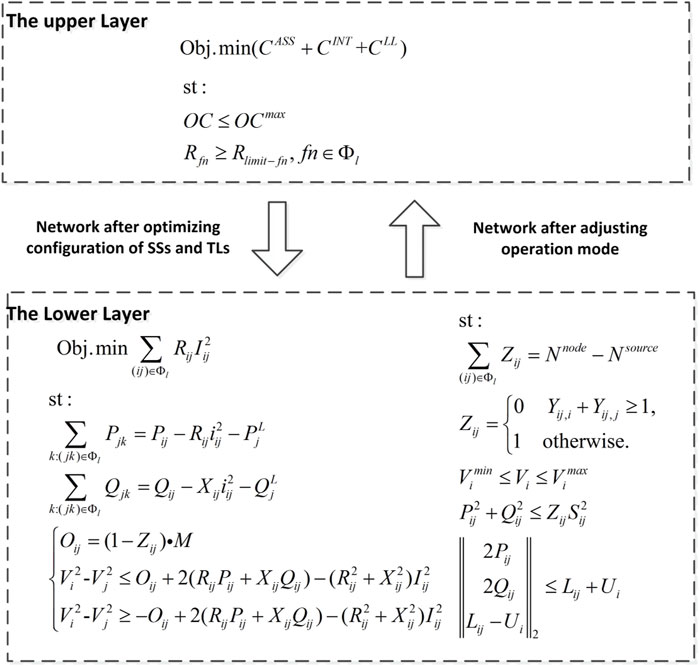
FIGURE 2. The proposed bi-level framework.

FIGURE 3

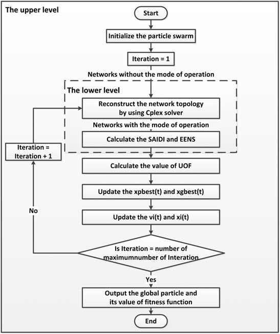
FIGURE 3. Bi-level optimization flow chart.

Step 1: Initialize the particle swarm based on the alternative locations of SSs and TLs.

Step 2: Transmit the network topology corresponding to the particle to the lower level.

Step 3: Reconstruct the network by using Cplex solver.

Step 4: Calculate the system reliability indexes and transmit these indexes back to the upper level.

Step 5: Calculate the value of the objective function.

Step 6: Update the local and global optimal particles.

Step 7:   Update the velocities and positions of the particle swarm.

Step 8:   If the iteration is over, output the global particle and its value of fitness function. Otherwise, return to Step 3.

4 Numerical Examples

The proposed bi-level model is applied to bus 2 and bus 4 of the modified Roy Billinton Test System (RBTS). In this section, the network data of the test system and other details of the simulations are provided thoroughly for the sake of reproducibility. Then, six case studies are conducted, and the results are comprehensively discussed. The proposed method for the SSs and TLs optimized planning is developed in MATLAB version R2018b and the simulations are carried out on a computer with Intel(R) Core (TM) i5-8400 CPU @ 2.8 GHz 2.81 GHz Processor and 8 GB of RAM.

4.1 Test Network and Simulation Assumptions

The bus 2 consists of 4 feeders, 36 feeder sections, and 22 load nodes, as represented in Figure 4. Also, 2 alternative TLs and a total of 28 alternative locations for the SSs are taken into account. Similarly, bus 4 is made up of 7 feeders, 67 feeder sections, 38 load nodes, 58 alternate positions of SSs, and 5 alternate positions of TLs, which was shown in Figure 5. The required data regarding reliability parameters, electrical parameters, and load data are derived from Billinton and Jonnavithula (1996). Table 2 represents the data for load nodes of bus 2. Table 3 presents the ratio between the load of the modified bus 4 in this paper and the load in Billinton and Jonnavithula (1996). The line length and the wire types of bus 2 are provided in Tables 4, 5, respectively.

FIGURE 4

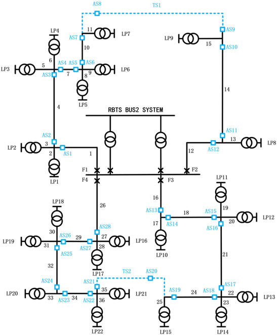
FIGURE 4. Bus 2 of the Roy Billinton test system.

FIGURE 5

FIGURE 5. Bus 4 of the Roy Billinton test system.

TABLE 2

TABLE 2. Data for bus 2 load nodes.

TABLE 3

TABLE 3. Data for bus 4 load ratios.

TABLE 4

TABLE 4. Length of Bus 2 lines.

TABLE 5

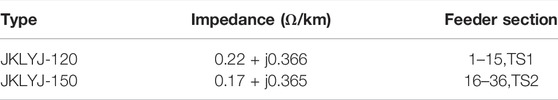
TABLE 5. Wire types and parameters of Bus 2 lines.

In the implemented simulations, all the SSs are assumed to be automatic and the switching duration of SSs is 1 min. The economic data for the alternative SSs and potential TLs are presented in Table 6. The investment recovery rate is set to 5%. The electricity average price and electricity price conversion multiples, $UC$ and $\chi$, are considered to be 0.13 $/kWh and 15, respectively. Meanwhile, it is assumed that the life span of equipment is 15 years with a constant annual load growth rate of 1.1%. Additionally, the reliability index R_limt-fn of 99.96% is used and the OC^max is infinite. Finally, Table 7 shows the specification of distribution fault type and the repair time of fault.

TABLE 6

TABLE 6. Economic data for SSs and TLs.

TABLE 7

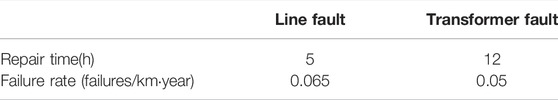
TABLE 7. Specifications of distribution fault type.

7In the lower-level model, the maximum number of iterations is 100, and the size of the particle population is 3,000. The value of particles' maximum velocity, the inertia weight, and the SSs configuration probability are 1.2, 0.9, and 0.15, respectively. The factors of learning and individual learning are 2.

4.2 Numerical Results of the Comparative Cases

Six cases are simulated to demonstrate the effectiveness of the proposed model as well as to show how considered operation mode adjustment provides advantages for the system.

Case I: This case provides information regarding the original network not installed with any SSs and TLs, which is a comparison benchmark to show the effectiveness of equipment deployment.

Case II: In this case, TLs are not allowed to be installed.

Case III: In this case, the TLs are installed after installing SSs.

Case IV :  The upper-level model is executed independently without the lower-level model in this case.

Case V:  Network reconstruction based on synchronous optimization of SSs and TLs

Case VI: The bi-model is carried out, considering the effect of operating mode adjustment on the coordination configuration of SSs and tie lies.

Table 8 summarizes various costs and EENS associated with Cases I to IV. Table 9 shows the device configuration results. Through comparison between Case I and Case II, the $C^{INT}$ in Case II is reduced by 37.28% due to the reduction of EENS. This shows that the deployment of SSs plays an important role in fault management and is essential to improving system reliability. To explore the effect of TLs, Case III examines how it can improve system reliability in the network already equipped with SSs. In Case III, it is obvious that the interruption cost falls from U.S. k$ 1,606.85 to U.S. k$ 887.61 (i.e., nearly a 45% reduction), despite the extra cost of U.S. k$ 100 due to the purchase of the TLs. Meanwhile, the line loss (LL) is reduced to 1.8% of the original network (from 866.77 MWh/year to 851.13 MWh/year) because it is assumed that the open-loop locations are the SSs closest to the TLs, which reduces the total cost to some extent. It can be seen that the network reconstruction could reduce the network line loss. Thus, the results associated with Case III can be considered as solutions for SSs placement, TLs deployment, and network reconstruction that are conventionally proceeded in sequence. Owing to the complementary effects of SSs and TLs in the fault management process, the placement of equipment may contribute to a more economical and efficient solution. In order to explore a better solution, Case IV takes simultaneous placement of all equipment into account. The total cost of U.S. k$ 2213.56 is imposed on the system, which is less than the total cost of Case III (sequential placement). The various costs are shown in Figure 6.

TABLE 8

TABLE 8. Cost of solutions of bus 2 for the six cases.

TABLE 9

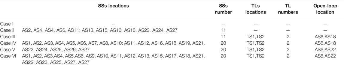
TABLE 9. The installation of bus 2 for the six cases.

FIGURE 6

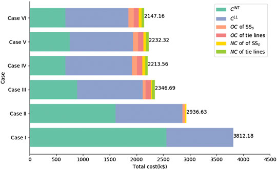
FIGURE 6. Cost in the six cases.

Compared with Case II, although the installation number of Case III does not increase, the EENS of the system after installing TLs is further reduced, as shown in Tables 8 and 9. The reason is that, without the installation of TLs, the SSs are limited to isolating the upstream load from the downstream fault and restoring the upstream load. However, with the installation of TLs, the function of SSs can not only restore upstream loads but also help transfer downstream loads. Therefore, the return on investment ratio of the SSs will be increased. Therefore, the optimal number of SSs for Case IV increased from 11 to 20 compared to Case III under the same constraints.

In order to further prove the impact of network reconfiguration on the total cost, network reconfiguration is conducted in Case V on the basis of Case IV. The results indicate that although the line loss of the distribution network is reduced by 45.39 MWh/year, the EENS increased by 12.4%, which lead to an increase in the total cost of the system. This means that the network reconfiguration with the objective function of minimizing the line loss may reduce the reliability of the distribution network operation and the total cost may not be the minimum. Therefore, in Case VI, the proposed method is developed.

As shown in Table 9, the number of installed SSs in Case IV, Case V, and Case VI are the same, and the number of TLs is also the same. Meanwhile, the network open-loop locations of Case VI and Case V are both AS6 and AS22, respectively, so their line losses are equal. Due to the different installation positions of the SSs, the EENS of Case VI is reduced by 12.55% as compared with Case V. The total cost is reduced by U.S. k$ 85.16. The total cost of Case VI is reduced by 43.68% compared to the total cost of the original network, which is the best among all the cases.

Likewise, these six cases are applied in bus 4, and the results are shown in Table 10. It can be seen that, compared to the original topology, SSs are installed in Case II. The total cost of Case II is reduced by 23% due to the reduction of customer interruption costs. Compared with Case II, TLs are allocated in Case III, which further reduces EENS and the total cost. However, the distribution network is not in optimal operation mode, and the line loss increases by 486.85 MWh/year, resulting in a rise in line loss cost. Similar to bus 2, the coordinated planning of SSs and TLs is conducted in Case IV, where the number of optimal SSs is larger than in Case III. With the distribution network reconfiguration, the line loss cost is further reduced in Case V. In Case VI, the proposed method in this paper is employed, achieving better network reliability and better operating economics at the lowest total cost. The detailed installation situation is shown in Tables 10, 11. Experimental results prove that the proposed model is likely to be robust enough for larger-scale networks.

TABLE 10

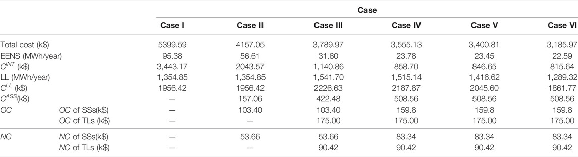
TABLE 10. Cost of solutions of bus 4 for the six cases.

TABLE 11

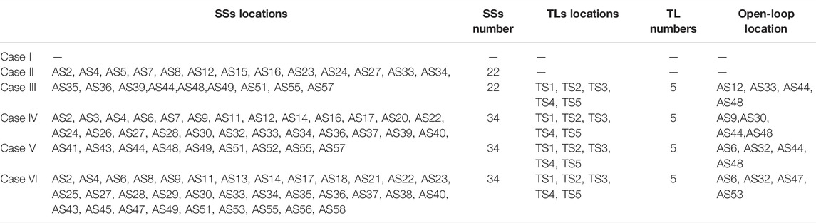
TABLE 11. The installation of bus 4 for the six cases.

Figure 7 and Figure 8 present the convergence characteristics as obtained by the proposed model for the bus 2 and bus 4, respectively. The results show that the best solution is obtained within a few iterations.

FIGURE 7

FIGURE 7. Convergence characteristic of the proposed model for bus 2

FIGURE 8

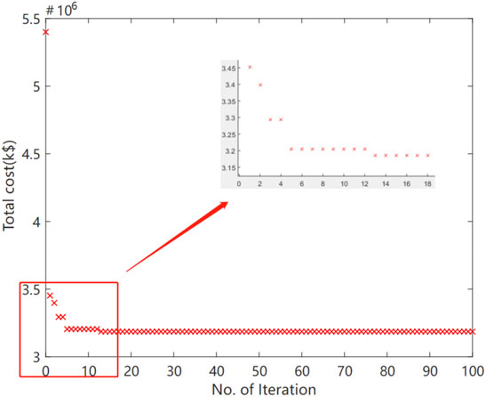
FIGURE 8. Convergence characteristic of the proposed model for bus 4

A Analysis on the effect of TLs on the SSs installation

In this subsection, only F1 and F2 are considered, and the 24 cases are divided into 12 groups. One case considered the installation of the TL TS1 and the other did not in each group. The group number indicates the number of installed SSs, and the installed SSs follow the rules of sequential installation. For example, Group I install a SS at AS1, Group II installs SSs at AS1 and AS2, and Group XII installs SSs at all alternative locations. Figure 9 provides the resultant cost and reliability indexes for the 24 cases.

FIGURE 9

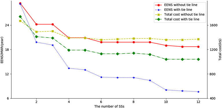
FIGURE 9. Resultant cost and reliability indexes in the 24 cases.

If the number of SSs installation is equal, the case with TLs has smaller EENS than the case without TLs, as well as the total cost. Moreover, with the number of SSs installed increasing, the EENS reduction in the case with TLs is larger than in the case without TLs. In particular, when the number of SSs increased to a certain number, the EENS of the case without TLs is slightly reduced, and the total cost increases accordingly. However, the case with TLs does not appear in this situation, which further demonstrates that the installation of the TLs improves the cost-benefit of the SSs installation.

B Analysis on the effect of network reconfiguration on the SSs installation

Likewise, this subsection only considers F1 and F2, with TL TS1 installed. Assuming that the open-loop location is from AS1 to AS12, different numbers of optimal switch combinations are enumerated to study the effect of open-loop location on SSs.

It can be seen from Table 12 that when the position of the open-loop point moves from AS1 to AS12, if the numbers of installed SSs are equal, the optimal SSs combinations are different, while some optimal SSs combinations are the same with open-loop points adjacent to each other. When the position of the open-loop point is fixed, the same characteristics of the optimal switch combination of adjacent open-loop points will continue to decline with the increase in the number of SSs. In addition, when the position of the open-loop point is fixed, with the increase of the number of installed SSs, the optimal SSs combination is not simply adding a new SS on the basis of the original low-order optimal SSs combination, but a different SSs combination. This means that the position of the open-loop point effectively affects the installation of the SSs.

TABLE 12

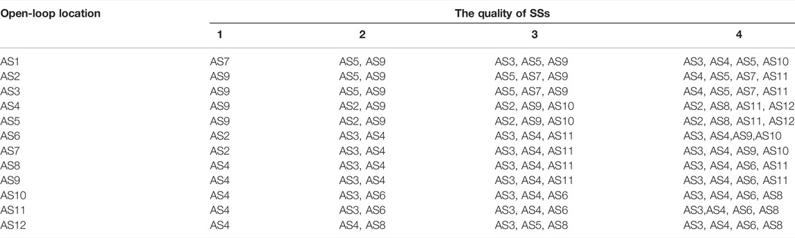
TABLE 12. The installation for the 48 cases.

5 Conclusion

This paper proposes a coordinated planning model for deploying SSs and TLs among distribution feeders, taking the adjustment of operating modes into account. The model is designed to minimize equipment costs, customer interruption costs, and line loss costs. The results obtained through the application of the test system and the related analysis demonstrated the integrity and effectiveness of the proposed model. The case studies have proved that the proposed method can achieve lower customer interruption loss, lower line loss, and higher economic benefits than the SSs configuration model, which provides a flexible planning scheme that is beneficial to power distribution systems by making more rational investment decisions. In future research, the configuration of distributed energy sources, SSs, and TLs in active distribution networks will be addressed.

Data Availability Statement

The raw data supporting the conclusion of this article will be made available by the authors, without undue reservation.

Author Contributions

Conceptualization, QL, CG, and XGP; methodology, QL, and WJL; software, CG and WJL; experiment, validation, and analysis, QL and CG; investigation, CG and JXZ; resources, XGP and PDC; data curation, QL, and ZHX; writing—original draft preparation, QL, and WJL; writing—review and editing, QL, LLL, XGP, and CSL. All authors have read and agreed to the published version of the manuscript.

Funding

This research was supported by the National Natural Science Foundation of China (61903091) and the Planning Project of Guangdong Power Grid Co., Ltd. (No. 031000QQ00210003).

Conflict of Interest

Authors QL, CG, JZ, PC, and ZX are employed by Planning Research of Guangdong Power Grid Co. Ltd. This study received funding from Planning Research of Guangdong Power Grid Co. Ltd. The funder had the following involvement with the study ‘Research on automatic generation strategy of medium voltage distribution network planning scheme (No. 031000QQ00210003).

The remaining authors declare that the research was conducted in the absence of any commercial or financial relationships that could be construed as a potential conflict of interest.

Publisher’s Note

All claims expressed in this article are solely those of the authors and do not necessarily represent those of their affiliated organizations, or those of the publisher, the editors, and the reviewers. Any product that may be evaluated in this article, or claim that may be made by its manufacturer, is not guaranteed or endorsed by the publisher.

References

Bezerra, J. R., Barroso, G. C., and Leão, R. P. (2014). Multiobjective Optimization Algorithm for Switch Placement in Radial Power Distribution Networks. IEEE Trans. Power Deliv. 30 (2), 545–552.

Google Scholar

Billinton, R., and Jonnavithula, S. (1996). Optimal Switching Device Placement in Radial Distribution Systems. IEEE Trans. Power Deliv. 11 (3), 1646–1651. doi:10.1109/61.517529

CrossRef Full Text | Google Scholar

Chen, Q., Wang, W., Wang, H., Wu, J., Li, X., and Lan, J. (2020). A Social Beetle Swarm Algorithm Based on Grey Target Decision-Making for a Multiobjective Distribution Network Reconfiguration Considering Partition of Time Intervals. IEEE Access 8, 204987–205013. doi:10.1109/access.2020.3036898

CrossRef Full Text | Google Scholar

De, A., Laura, S., and Vizcaino, G. (2014). Switch Allocation Problems in Power Distribution Systems. IEEE Trans. Power Syst. 30 (1), 246–253.

Google Scholar

Du, P., Chen, Z., Chen, Y., Ma, Z., and Ding, H. (2019). A Bi-level Linearized Dispatching Model of Active Distribution Network with Multi-Stakeholder Participation Based on Analytical Target Cascading. IEEE Access 7, 154844–154858. doi:10.1109/access.2019.2949097

CrossRef Full Text | Google Scholar

Falaghi, H., Haghifam, M. R., and Singh, C. (2008). Ant Colony Optimization-Based Method for Placement of Sectionalizing Switches in Distribution Networks Using a Fuzzy Multiobjective Approach. IEEE Trans. Power Deliv. 24 (1), 268–276.

Google Scholar

Falaghi, H., Haghifam, M. R., and Singh, C. (2008). Ant Colony Optimization-Based Method for Placement of Sectionalizing Switches in Distribution Networks Using a Fuzzy Multiobjective Approach. IEEE Trans. Power Deliv. 24 (1), 268–276.

Google Scholar

Farivar, M., and Low, S. H. (2013). Branch Flow Model: Relaxations and Convexification-Part I. IEEE Trans. Power Syst. 28 (3), 2554–2564. doi:10.1109/tpwrs.2013.2255317

CrossRef Full Text | Google Scholar

Fernandez-Martinez, J. L., and Garcia-Gonzalo, E. (2011). Stochastic Stability Analysis of the Linear Continuous and Discrete PSO Models. IEEE Trans. Evol. Computat.June 15 (3), 405–423. doi:10.1109/tevc.2010.2053935

CrossRef Full Text | Google Scholar

Fumagalli, E., Schiavo, L., and Delestre, F. (2007). Service Quality Regulation in Electricity Distribution and Retail. Springer Science & Business Media.

Google Scholar

Gholizadeh, N., Hosseinian, S. H., Abedi, M., Nafisi, H., and Siano, P. (2022). Optimal Placement of Fuses and Switches in Active Distribution Networks Using Value-Based MINLP. Reliab. Eng. Syst. Saf. 217, 108075. doi:10.1016/j.ress.2021.108075

CrossRef Full Text | Google Scholar

Heidari, A., Agelidis, V. G., and Kia, M. (2014). Considerations of Sectionalizing Switches in Distribution Networks with Distributed Generation. IEEE Trans. Power Deliv. 30 (3), 1401–1409.

Google Scholar

Heidari, A., Agelidis, V. G., and Kia, M. (2016). Reliability Optimization of Automated Distribution Networks with Probability Customer Interruption Cost Model in the Presence of DG Units. IEEE Trans. Smart Grid 8 (1), 305–315.

Google Scholar

Heidari, A., Dong, Z. Y., and Zhang, D. (2017). Mixed-integer Nonlinear Programming Formulation for Distribution Networks Reliability Optimization. IEEE Trans. Industrial Inf. 14 (5), 1952–1961.

Google Scholar

Hsu, Y.-Y., Yi, J.-H., Liu, S. S., Chen, Y. W., Feng, H. C., and Lee, Y. M. (1993). Transformer and Feeder Load Balancing Using a Heuristic Search Approach. IEEE Trans. Power Syst. 8 (1), 184–190. doi:10.1109/59.221264

CrossRef Full Text | Google Scholar

Jooshaki, M., Abbaspour, A., Fotuhi-Firuzabad, M., Moeini-Aghtaie, M., and Lehtonen, M. (2019). MILP Model of Electricity Distribution System Expansion Planning Considering Incentive Reliability Regulations. IEEE Trans. Power Syst. 34 (6), 4300–4316. doi:10.1109/tpwrs.2019.2914516

CrossRef Full Text | Google Scholar

Karimi, H., Niknam, T., Dehghani, M., Ghiasi, M., Ghasemigarpachi, M., Padmanaban, S., et al. (2021). Automated Distribution Networks Reliability Optimization in the Presence of DG Units Considering Probability Customer Interruption: A Practical Case Study. IEEE Access 9, 98490–98505. doi:10.1109/access.2021.3096128

CrossRef Full Text | Google Scholar

Lee, J., Lee, H., and Nah, W. (2022). Minimizing the Number of X/Y Capacitors in an Autonomous Emergency Brake System Using the BPSO Algorithm. IEEE Trans. Power Electron. 37 (2), 1630–1640. doi:10.1109/tpel.2022.3167941

CrossRef Full Text | Google Scholar

Lei, S., Wang, J., and Hou, Y. (2017). Remote-controlled Switch Allocation Enabling Prompt Restoration of Distribution Systems. IEEE Trans. Power Syst. 33 (3), 3129–3142.

Google Scholar

Li, B., Wei, J., Liang, Y., and Chen, B. (2020). Optimal Placement of Fault Indicator and Sectionalizing Switch in Distribution Networks. IEEE Access 8, 17619–17631. Jan. doi:10.1109/access.2020.2968092

CrossRef Full Text | Google Scholar

Li, Y., Xiao, J., Chen, C., Tan, Y., and Cao, Y. (2019). Service Restoration Model with Mixed-Integer Second-Order Cone Programming for Distribution Network with Distributed Generations. IEEE Trans. Smart Grid 10 (4), 4138–4150. doi:10.1109/tsg.2018.2850358

CrossRef Full Text | Google Scholar

Li, Z., Wu, W., Tai, X., and Zhang, B. (2020). Optimization Model-Based Reliability Assessment for Distribution Networks Considering Detailed Placement of Circuit Breakers and Switches. IEEE Trans. Power Syst. 35 (5), 3991–4004. doi:10.1109/tpwrs.2020.2981508

CrossRef Full Text | Google Scholar

Liao, Y. Q., Zhang, J., and Wang, Z. D. (2018). Three Stage Optimization Algorithm for Medium Voltage Overhead Line Switch Configuration. Power Grid Technol. 42, 3413–3419.

Google Scholar

Lin, Z., Hu, Z., and Song, Y. (2019). Distribution Network Expansion Planning Considering $N-1$ Criterion. IEEE Trans. Power Syst. 34 (3), 2476–2478. doi:10.1109/tpwrs.2019.2896841

CrossRef Full Text | Google Scholar

Miranda, V., Ranito, J. V., and Proenca, L. M. (1994). Genetic Algorithms in Optimal Multistage Distribution Network Planning. IEEE Trans. Power Syst.Nov 9 (4), 1927–1933. doi:10.1109/59.331452

CrossRef Full Text | Google Scholar

Munoz-Delgado, G., Contreras, J., and Arroyo, J. M. (2017). Distribution Network Expansion Planning with an Explicit Formulation for Reliability Assessment. IEEE Trans. Power Syst. 33 (3), 2583–2596.

Google Scholar

Nguyen, B. H., Xue, B., Andreae, P., and Zhang, M. (2019). A New Binary Particle Swarm Optimization Approach: Momentum and Dynamic Balance between Exploration and Exploitation. IEEE Trans. Cybern. PP (2), 589–603. doi:10.1109/TCYB.2019.2944141

PubMed Abstract | CrossRef Full Text | Google Scholar

Popovic, Z., Brbaklic, B., and Knezevic, S. (2017). A Mixed Integer Linear Programming Based Approach for Optimal Placement of Different Types of Automation Devices in Distribution Networks[J]. Electr. Power Syst. Res. 148, 136–146.

Google Scholar

Ray, S., Bhattacharya, A., and Bhattacharjee, S. (2016). Optimal Placement of Switches in a Radial Distribution Network for Reliability Improvement. Int. J. Electr. Power & Energy Syst. 76, 53–68. doi:10.1016/j.ijepes.2015.09.022

CrossRef Full Text | Google Scholar

Sahoo, N. C., Ganguly, S., and Das, D. (2012). Multi-objective Planning of Electrical Distribution Systems Incorporating Sectionalizing Switches and Tie-Lines Using Particle Swarm Optimization. Swarm Evol. Comput. 3, 15–32. doi:10.1016/j.swevo.2011.11.002

CrossRef Full Text | Google Scholar

Sannigrahi, S., Ghatak, S. R., and Acharjee, P. (2019). Multi-scenario Based Bi-level Coordinated Planning of Active Distribution System under Uncertain Environment. IEEE Trans. Industry Appl. 56 (1), 850–863.

Google Scholar

Shojaei, F., Rastegar, M., and Dabbaghjamanesh, M. (2020). Simultaneous Placement of Tie-Lines and Distributed Generations to Optimize Distribution System Post-outage Operations and Minimize Energy Losses. CSEE J. Power Energy Syst. 7 (2), 318–328.

Google Scholar

Skoonpong, A., and Sirisumrannukul, S. (2008). “Network Reconfiguration for Reliability Worth Enhancement in Distribution Systems by Simulated Annealing,” in 2008 5th International Conference on Electrical Engineering/Electronics, Computer, Telecommunications and Information Technology, 2, 937–940.

CrossRef Full Text | Google Scholar

Velasquez, M. A., Quijano, N., and Cadena, A. I. (2016). Optimal Placement of Switches on DG Enhanced Feeders with Short Circuit Constraints. Electr. Power Syst. Res. 141, 221–232. doi:10.1016/j.epsr.2016.08.001

CrossRef Full Text | Google Scholar

Wang, B., Zhu, H., Xu, H., Bao, Y., and Di, H. (2021). Distribution Network Reconfiguration Based on NoisyNet Deep Q-Learning Network. IEEE Access 9, 90358–90365. doi:10.1109/access.2021.3089625

CrossRef Full Text | Google Scholar

Xu, Y., Zhang, J., Wang, P., and Lu, M. (2021). Research on the Bi-level Optimization Model of Distribution Network Based on Distributed Cooperative Control. IEEE Access 9, 11798–11810. doi:10.1109/access.2021.3051464

CrossRef Full Text | Google Scholar

Zhang, L., Xuedong, P. A., and Haoran, Z. H. (2019). “Bi-level Expansion Planning Method for Active Distribution Network Considering Dynamic Network Reconfiguration,” in 2019 IEEE Sustainable Power and Energy Conference, 1984–1989. doi:10.1109/ispec48194.2019.8975158

CrossRef Full Text | Google Scholar

Zhong, T., Zhang, H. T., and Li, Y. (2020). Bayesian Learning-Based Multi-Objective Distribution Power Network Reconfiguration. IEEE Trans. Smart Grid 12 (2), 1174–1184. doi:10.1109/tsg.2020.3027290

CrossRef Full Text | Google Scholar

Nomenclature

Indices

ft Number of failure types

lp Time

lf Fault location in line

pf Fault location in load node

ct Type of customer

fn Number of feeders

pn Number of load point

tf Fault location

i/j/k Node i, node j, and node k of the distribution network

ij Branch from node i to node j

Variables

R Branch resistance

X Branch reactance

P Active power at the head of branch

P^L Net outflow active power of node

Q Reactive power at the head of branch

Q^L Net outflow reactive power of node

S Apparent power

V Node voltage

I Branch current

U The square of the node voltage

L The square of the branch current

Sets

${\mathit{\Phi }}_{\mathit{l}}$ Set of all branches in the distribution network

${\mathit{\Phi }}_{\mathit{f}\mathit{n}}$ Set of all feeders in the distribution network

Parameters

PC_SS, PC_TL The unit purchase cost of SS and TL [$]

IC_SS, IC_TL The unit installation cost of SS and TL [$]

CC Customer outage cost[$]

UC Customer outage unit cost[$/kWh]

LC Line loss unit cost[$/kWh]

TR Outage duration[h]

PR Electricity consumption or production in load nodes [kW]

β Average failure rate of device

μ Inflation rate

γ Annual load increment rate

δ The rate of SSs’ annual operation and maintenance cost to SSs’ purchase cost

χ Price conversion coefficient

OC^max Maximum cost of one-time investment

N^lp Life period of equipment

N^tf Total number of all failure locations

N^tl Total number of all alternative TLs

N^fn Total number of feeders

N^pn Total number of load points

N^pf Total number of failures in load point

N^lf Total number of failures in line

N^ft Total number of fault types

N^max Maximum number of switches to be installed

V^min Minimum voltage threshold

V^max Maximum voltage threshold