Abstract
In recent years, data-driven methods have shown great potential for the practical application of short-term voltage stability (STVS) assessment. However, most existing research works overlook the problem of sample imbalance and overlap in STVS assessment. To tackle this issue, a novel self-adaptive data-driven method for real-time STVS is proposed in this study. First, min-redundancy and max-relevance (mRMR) is employed for feature selection to reduce the computational burden. Taking the key features as inputs, a cascaded LightGBM (CasLightGBM) model is constructed to mine STVS informatization. Based on the LightGBM and cascaded structure, CasLightGBM can enhance the assessment accuracy without sacrificing the assessment earliness. Then, focal loss (FL) is embedded into both offline and online phases of the CasLightGBM to mitigate the loss of accuracy caused by sample imbalance and overlapping, thus deriving a highly comprehensive and reliable classification model for real-time STVS assessment. Extensive numerical tests are conducted on the IEEE 118-bus system, and the simulation results demonstrate that the proposed method outperforms traditional algorithms and exhibits favorable robustness to measurement noise.
Introduction
With the large-scale integration of renewable energy and the continuous growth of power consumption, the secure and reliable operation of modern power systems is facing serious challenges (Li S. et al., 2021; Li Z. et al., 2021; Ma et al., 2021). As a major threat to the stability of power systems, the consequence of short-term voltage instability may result in voltage collapse and even widespread blackouts (Dong et al., 2016; Zhu et al., 2020), such as the Athens blackout in 2004 (Vournas et al., 2006) and the South Australia blackout in 2016 (Yan et al., 2018). Therefore, an accurate, real-time, and reliable evaluation method for short-term voltage stability (STVS) is urgently required, which contributes to taking remedial control actions in a timely manner to avoid potential accidents.
Traditionally, numerical analysis methods have been used for voltage stability assessments based on time-domain simulations (TDS) and Lyapunov exponents. TDS can calculate a reliable solution, but it relies on iteratively solving a large number of differential-algebraic equations, which is computationally expensive and impractical for real-time STVS assessment. STVS analysis using the Lyapunov exponent for a certain time window is proposed by Dasgupta et al. (2013). However, there are still no effective methods to obtain accurate model parameters, which may suffer from numerical problems in large-scale power systems.
Recently, with the wide deployment of wide-area measurements (WAMS), a huge amount of dynamics monitoring data obtained from dispersive phasor measurement units (PMUs) are available (De La Ree et al., 2010; Fernandes et al., 2017; He et al., 2017). Owing to real-time PMU data, data-driven machine learning (ML) methods can be adequately leveraged to explore online STVS schemes. In Diao et al. (2009) and Zhu et al. (2017), a decision tree (DT) has been used for STVS assessment, and in Yang et al. (2018) a support vector machine (SVM)–based method is applied for online STVS analysis. Nevertheless, it is difficult for DT and SVM to fit complex dynamic response functions with high accuracy due to the simple network structure. To improve the generalization ability, the works by Zhang et al. (2019a) and Zhang et al. (2019b) present a hierarchical assessment approach using an ensemble of extreme learning machines (ELMs) and artificial neural networks (ANNs), respectively. The ensemble models improve the prediction accuracy by integrating weak learners, but they are prone to overfitting. In Rizvi et al.’s (2021) study, a new approach based on a convolutional neural network (CNN) is introduced for STVS assessment considering data anomalies and fault localization. Moreover, the long-short-term-memory network (LSTM) is used to extract voltage stability information from the time-varying features in Zhang et al. (2021). Combined with the spatial-temporal characteristics, the deep graph neural network proposed by Luo et al. (2021) and Zhong et al. (2022) has shown higher accuracy and better adaptability. The deep learning algorithms in Luo et al. (2021), Rizvi et al. (2021), Zhang et al. (2021), and Zhong et al. (2022) can establish an excellent input–output mapping relationship, but problems such as large demand for data samples and long training time remain to be solved.
Moreover, the aforementioned typical ML-based STVS assessment approaches have some severe limitations, for example, they do not consider the impact of sample imbalance on STVS feature learning. For practical large-scale power grids, with the help of increasingly perfect relay protection devices, the system can remain stable after most disturbances, and becomes unstable only in the terrible rare scenarios. If not treated properly, this phenomenon would dramatically deteriorate the model’s attention to unstable samples. Consequently, the unstable samples tend to be overlooked by the trained model and thus misclassified. Meanwhile, misclassification of unstable scenarios would lead to cascade faults or catastrophic voltage collapse because appropriate emergency control measures cannot be taken in time. Relatively speaking, misdetection of power system stability is usually remediable with much less expense. To modify the tendency of the ML-based model, a reconstruction residual-based STVS assessment method is adopted by Yang et al. (2020). This method uses LSTM and fully connected layers to build an autoencoder, and then the reconstruction residual of the autoencoder is utilized for indicating STVS, which is effective but computationally complex. In addition, another crucial imperfection is that the classification difficulty of samples in overlapping regions is neglected. Similar to the sample imbalance problem, this phenomenon would also damage the prediction accuracy of the machine learning model.
Given all the aforementioned concerns, this study proposes a self-adaptive data-driven method to improve the comprehensiveness and reliability of STVS assessments. It mitigates computational burden by a cascaded LightGBM (CasLightGBM) and introduces the focal loss (FL) (
Lin et al., 2020) as a new loss function in the CasLightGBM training to modify attention for imbalanced samples and overlapping samples. In addition, min-redundancy and max-relevance (mRMR) is employed for feature selection, so as to reduce the computational burden. The main contributions and merits of this study include the following.
1) A novel data-driven approach based on the CasLightGBM is constructed for STVS assessment. Based on LightGBM and cascaded structure, CasLightGBM can enhance the assessment accuracy without sacrificing the assessment earliness.
2) In order to modify the incorrect tendency of the model in the training phases, FL is introduced to improve CasLightGBM, so the accuracy loss caused by sample imbalance and overlap can be mitigated.
3) The proposed method is validated on the IEEE 118-bus system and compared against other ML models. The simulation results demonstrate that the proposed method outperforms traditional algorithms and exhibits favorable robustness to measurement noise.
Problem Description
Short-Term Voltage Stability
Short-term voltage stability refers to the ability of the power system to rapidly recover an acceptable voltage level after a large disturbance (Kundur et al., 2004; Glavic et al., 2012). The typical post-disturbance voltage trajectories are illustrated in Figure 1 and Figure 2. In the stable scenario, the voltages of all buses can recover to an acceptable level (i.e., no less than 0.90 p.u voltage levels) after the disturbance is cleared (Zhang et al., 2019c; Ren et al., 2020; Zhu et al., 2021). In contrast, if any bus voltage remains at a low level or voltage collapses within a short-term time period, the power system is considered to be unstable, which may lead to cascading failures or even large-scale blackouts.
FIGURE 1
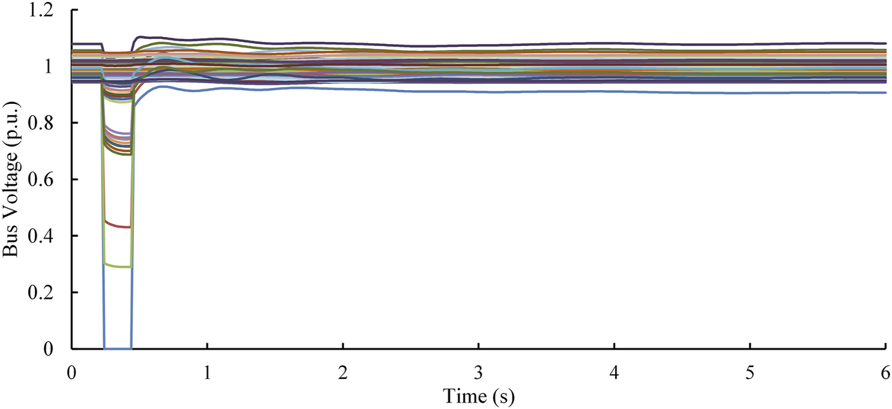
Example of stable scenario.
FIGURE 2
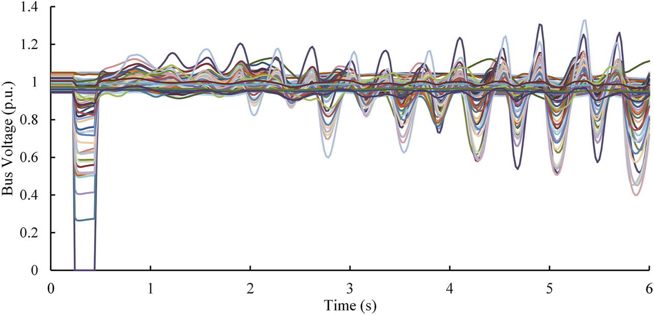
Example of unstable scenario.
Original Features
The input features determine the upper limit of machine learning evaluation performance. The richer the voltage steady status information contained in the input features, the more conducive it is to machine learning to accurately characterize complex power system dynamic response functions. Therefore, the original input characteristics should fully reflect the operating state of the power system and include the key factors affecting the transient voltage stability. For short-term voltage instability, the main reason is the insufficient dynamic reactive power support capability of the power system. In addition, active power is also associated with voltage instability (Liu et al., 2017; Vanfretti and Arava, 2020). According to Liu et al. (2017), Vanfretti and Arava (2020), and Zhu et al. (2021), the important influence variables (shown in Table 1) that are available in PMU are selected to form the initial feature vectors.
TABLE 1
| No. | Feature description | No. | Feature description |
|---|---|---|---|
| 1 | Node voltage amplitude | 5 | Load reactive power |
| 2 | Generator active power | 6 | Branch active power flow |
| 3 | Generator reactive power | 7 | Branch reactive power flow |
| 4 | Load active power |
Original features of TVSA.
Short-Term Voltage Stability Assessment Based on CasLightGBM
CasLightGBM
LightGBM is an algorithm framework based on the gradient boosting decision tree (GBDT) (Ke et al., 2017), which approximates the final model by integrating the CART regression tree. We assumed that a given dataset is D = {(xi, yi)|i = 1, 2,..., n}, where there are n samples, and each sample xi has m features. In the iteration of LightGBM, it is supposed there are T regression trees used to build the model.where ft is the tth regression tree and is the set space of all trees.
LightGBM uses the Newton method to quickly approximate the objective function, and trains the model in the additive form to get:where gi and hi are the first-order and second-order values of the loss function, respectively.
During the training process, LightGBM speeds up the establishment of each decision tree through the histogram algorithm and the leaf-wise strategy with depth limitation, thereby effectively shortening the training time. In order to further improve the ability of LightGBM to characterize high-dimensional and strong nonlinear complex power system functions, and to realize the layer-by-layer expression learning of input features, this study constructs the cascaded LightGBM by referring to the deep forest framework (Zhou and Feng, 2017). Deep forest achieves the multi-layer expression effect of the deep learning structure through the layer-by-layer series random forest, and has high computing efficiency, which provides a new idea for further improving the prediction accuracy of the model. LightGBM has lower memory consumption and better generalization ability than random forest. Therefore, this study utilizes CasLightGBM to replace the cascading forest structure, as shown in Figure 3.
FIGURE 3
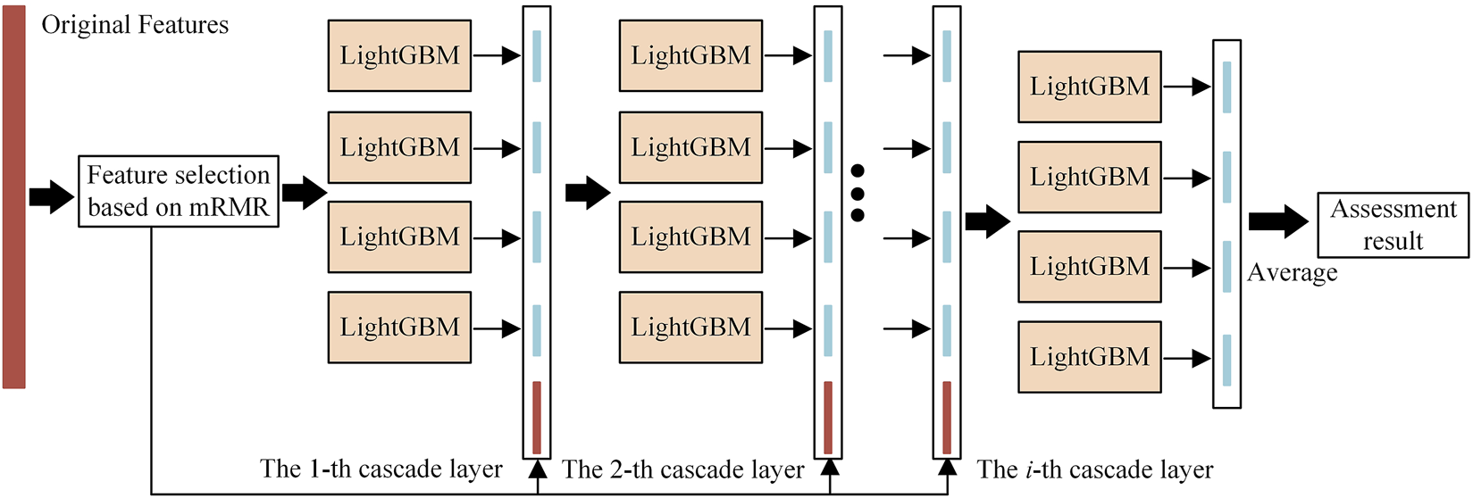
The structure of CasLightGBM.
The cascade layer of CasLightGBM is composed of four different LightGBM learners. During the establishment of CasLightGBM, the geometric mean (Gmean) is adopted as the indicator to judge whether the cascade layers need to be added, and it is given by Eq. 3:where TPR is the percentage of stable samples that are correctly classified and TNR is the percentage of unstable samples that are correctly classified.
When CasLightGBM expands a new cascade layer, it is judged whether the calculated Gmean of the current layer is greater than that of the previous layer, and the cascade layer will continue to expand if the requirement is met.
Focal Loss Function
For binary classification tasks, the loss function of the model usually chooses the cross-entropy (CE) function:where y represents the short-term voltage steady status, and p is the predicted probability corresponding to the stable sample (y = 1) or the unstable sample (y = 0). For notational convenience, pt is defined as follows:
Substituting Eq. 5 into Eq. 4 presents:
It can be seen from Eq. 6 that the closer pt is to 1, the smaller the value of CE(pt); conversely, the larger the value of CE(pt).
During the operation of the power system, the number of stable samples will be much larger than the number of unstable samples. The total loss of massive unstable samples is much larger than the stable samples, making CasLightGBM pay more attention to stable samples during the training process while ignoring the unstable samples that have important reference significance for triggering control devices. At the same time, if the voltage stability is misjudged, it is easy to induce cascade faults and even cause voltage collapse because appropriate emergency control measures cannot be taken in time. Therefore, the weight factor αt is introduced in CE to assign different weights to the two classes of samples. For notational convenience, αt is defined as follows:
The loss function with the weight factor αt is shown in Eq. 8:
Eq. 8 balances the distribution difference and importance of stable samples and unstable samples, but does not consider the difficulty of sample classification in overlapping regions. The samples that are difficult to classify are located in the overlapping area near the stable boundary in the feature vector space, and the probability of being misclassified is greater. Conversely, the samples that are easy to learn and classify are in non-overlapping regions with larger pt and smaller loss values. However, the cumulative loss value of the easily classified samples is large, which is a major contribution to the loss function and dominates the updating direction of the gradient, making the model ignore the transient voltage information contained in the difficult-to-classify samples during the iteration process and cannot reliably identify them. Therefore, a modulating factor (1-pt)γ is added to BCE(pt) to adjust the attention of the model to samples with different classification difficulties, as shown in Eq. 9:
In the iterative process, the model pays more attention to difficult-to-classify samples and learns them efficiently by adjusting the direction of the gradient optimization. It should be noted that the magnitude of the modulating factor changes dynamically. As the iteration progresses, the discrimination difficulty of the hard-to-classify samples decreases, the pt gradually increases, and the values of the modulation factor and loss value also decrease.
The introduction of FL(pt) into CasLightGBM not only resolves the negative impact of sample imbalance, but also strengthens the attention of the model to samples in overlapping regions, which is more helpful in accurately predicting the risk of short-term voltage instability.
Short-Term Voltage Stability Assessment Framework
The flowchart of the CasLightGBM-based STVS assessment method is proposed in Figure 4. The scheme consists of four stages, namely, data preparation, feature selection, offline CasLightGBM training, and online assessment and update.
FIGURE 4
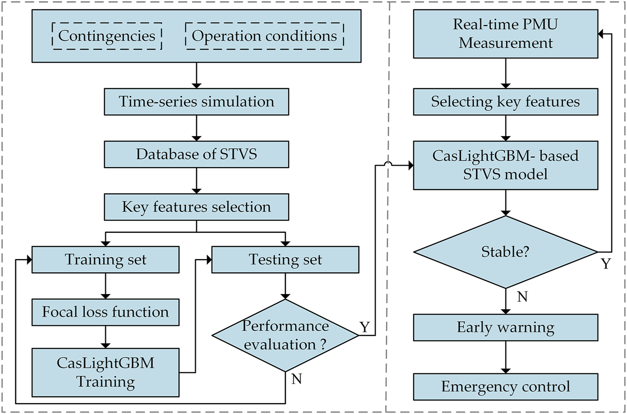
The framework of the proposed approach.
Data Preparation
To evaluate real-time voltage stability, first, a reliable and abundant database should be prepared. The database can be generated by using a time-series simulation of defined contingencies (e.g., three-phase faults) on the given power system, and some possible typical operating conditions are considered. In addition, the transient operation cases of the researched system can also be extensively collected to obtain the data required for model offline training.
Feature Selection
The operation variables that can reflect STVS are chosen to construct the input features, including node voltage amplitude, generator reactive power, generator reactive power, load active power, load reactive power, branch active power flow, and branch reactive power flow. Since the number of operation variables increases dramatically as the system scale expands, it is extremely stressful for subsequent CasLightgGBM training calculations. Therefore, it is necessary to extract key features from the initial feature set.
mRMR is a feature selection method based on mutual information, which maximizes the correlation between the input features and the result features while also considering the redundancy between the input features (Peng et al., 2005). In order to reduce the complexity of the model and accelerate the training time, mRMR is introduced to screen the strong representational features with low dimensionality from the original high-dimensional features.
The mutual information I(S; Y) between feature S and feature Y is defined as follows:where p(s) and p(y) are the marginal probability distribution function of s and y, respectively; p(s, y) represents the joint probability density function of s and y.
The objective of feature selection using mRMR is to maximize the correlation between the selected features S and the voltage steady status Y and minimize the redundancy between the selected features.where Si is the ith feature of the selected feature subset S and |S| is the dimension of feature subset S.
Combining Eq. 11 and Eq. 12, the feature selection criteria can be obtained as follows:
Based on the feature selection criteria, mRMR uses an incremental search method to find the key feature subset. Assuming that m-1 key features have been obtained, the mth feature is selected from the remaining features and satisfies the following equation:
For notational convenience, the obtained key features set is defined as follows:
Offline CasLightGBM Training
The prepared data are utilized to iteratively train CasLightGBM, and then establish the mapping relationship between the key features and transient voltage stability status in a data-driven manner. During model training, the optimal values of the weight factor α and parameter γ in the FL function are determined. To effectively evaluate the performance of CasLightGBM, the confusion matrix in Table 2 is used to define more evaluation indicators, which include accuracy (Acc), TPR, TNR, and Gmean (shown in Eq. 3).
TABLE 2
| Predicted stable | Predicted unstable | |
|---|---|---|
| Actual stable | TP | FN |
| Actual unstable | FP | TN |
Confusion matrix.
Online Assessment and Update
After meeting the performance requirements, the obtained CasLightGBM can be efficiently applied to the online SVS assessment. The real-time measurements of the corresponding key features are obtained from the PMU, and then the STVS status is immediately predicted by CasLightGBM after the fault is cleared. If the system is assessed as unstable, an early warning is given to the dispatchers immediately, so they can plan an emergency control strategy more quickly to maintain the safe and stable operation of the system.
After that, the monitoring PMU data are fed back to the original database for subsequent dynamic updates of CasLightGBM, so as to further improve the generalization ability and adaptability of the proposed method.
Case Study
The proposed CasLightGBM-based STVS assessment method is tested on the IEEE 118-bus system (shown in Figure 5), which has 118 buses, 54 thermal units, and 91 loads. The test is conducted on a computer equipped with an Intel Core i7 CPU working at 3.3-GHz and 16-GB RAM. The transient simulation is performed using commercial software PSS/E, and the machine learning methods are implemented in the Python platform.
FIGURE 5
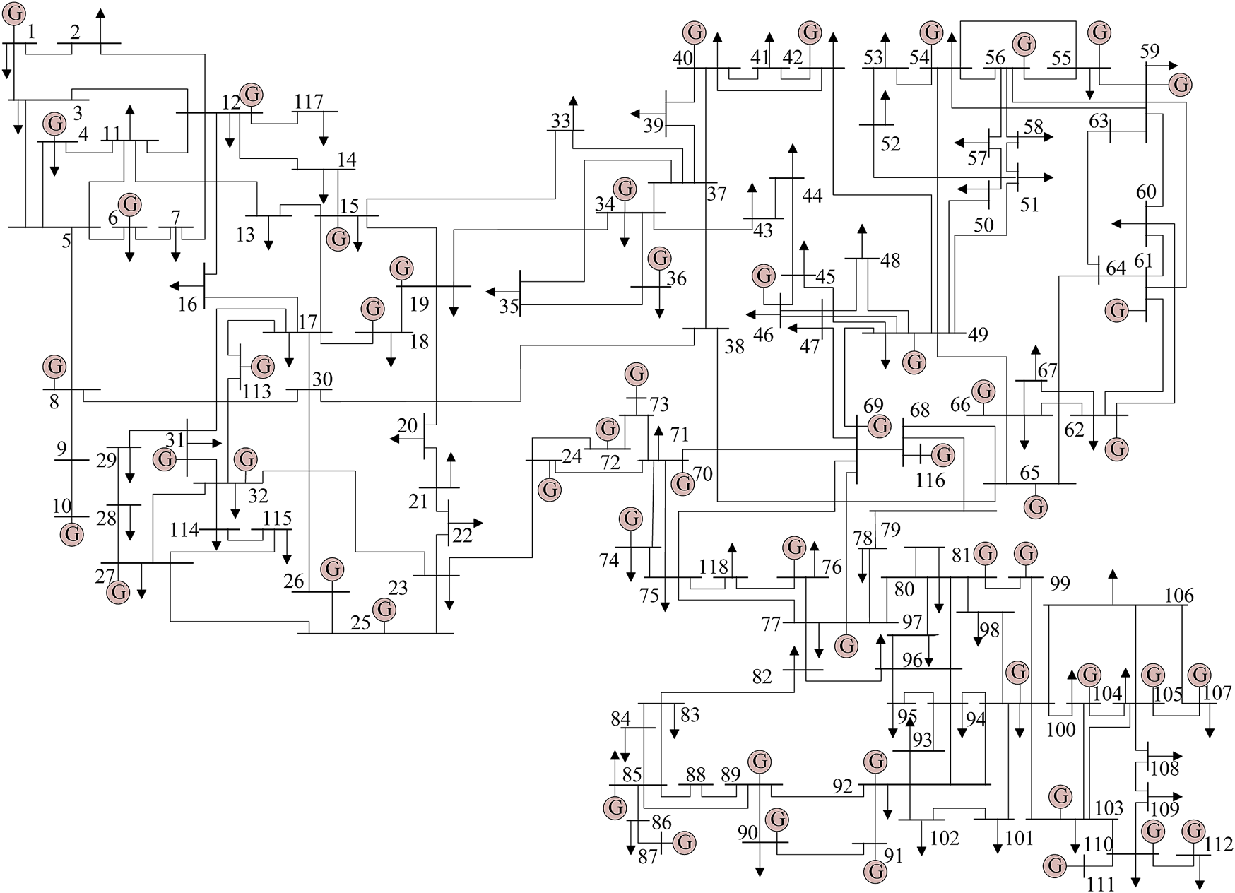
Topology of the IEEE 118-bus system.
Database Generation
To obtain a comprehensive database, a wide variety of operating conditions are considered. Considering the load level ranging from 75 to 125% of its base values, the power output of the generators was adjusted accordingly. For each load level, the three-phase grounding faults are created to occur on all buses and all transmission lines, where the faults are located at 0, 25, 50, and 70% of the length. In addition, the fault duration for each operating scenario is selected at 0.1 and 0.2 s. Each simulation is carried out for a time of 10 s. Based on the aforementioned configurations, 7,445 cases were generated via numerical simulations, with each one being carried out for 10 s to determine its STVS status. In particular, if the monitored voltages of all buses can successfully recover an acceptable equilibrium (i.e., no less than 0.90 p.u voltage levels) within the maximum simulation time, the produced case would be considered as stable, otherwise unstable.
Effect of Key Feature Number on Evaluation Performance
For the initial database, 806 operation features are extracted from the simulation results in the IEEE 118-bus system. To reduce the unnecessary computational burden, mRMR is introduced to select the important features. Figure 6 shows the impact of the selected key features on the evaluation indices. With the increase of the key features, the evaluation indices (i.e., Acc, TPR, TNR, and Gmean) of the proposed method have been significantly improved, and gradually tend to be smooth and steady. When the amount of the selected key features is 201, the highest Acc, TPR, TNR, and Gmean can be acquired. Therefore, the first 201 key features extracted by the mRMR are determined as new input features. The dimension of the important features is 24.94% of the initial features, which significantly reduces the computational burden of CaslightGBM while ensuring excellent evaluation performance.
FIGURE 6
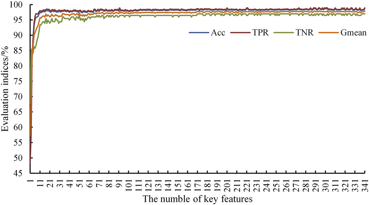
Impact of the number of key features on classification performance.
Effect of α and γ
In this section, the values of α and γ in the FL function are changed to enhance the attention distribution of CasLightGBM during the training process thereby improving the fitting degree of CasLightGBM to unstable samples and difficult-to-classify samples. The effect of different α values on the evaluation performance of CasLightGBM is shown in Figure 7.
FIGURE 7
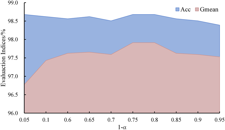
Evaluation performance of the model in different (1-α) values.
When the value of (1-α) is in the range of [0, 0.75], Gmean shows an obvious upward trend, and Acc does not decrease significantly. When the value of (1-α) is 0.75, the obtained Gmean is optimal, and the model has the best-imbalanced sample processing capability. It should be noted that too large a value of (1-α) will also destroy the balance between stable sample information and unstable sample information processed by CaslightGBM, resulting in the decline of its prediction performance.
Figure 8 shows the results of different γ values for STVS assessment using the proposed method. As shown in Figure 8, the best Gmean and Acc can be obtained when γ = 4. The modulating factor can further improve the fitting degree of the model to difficult-to-classify samples. Compared with the case of γ = 0, the Gmean increases by 1.17%.
FIGURE 8
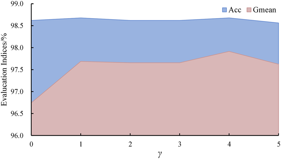
Evaluation performance of the model in different γ values.
Comparison With Other Methods
To further demonstrate the superiority of the proposed method, four other methods, including LightgGBM, LSTM (Zhang et al., 2021), 1D-CNN (Rizvi et al., 2021), DT, and ANN, are selected for comparison. Table 3 compares the classification performance of the proposed CasLightGBM with other machine learning methods. Combined with the cascaded structure and FL function, the evaluation performance of CasLightGBM is effectively improved. Leveraging CasLightGBM, the acquired TNR and Gmean are 2.04 and 0.94% more than LightgGBM, respectively. LSTM and 1D-CNN can effectively mine voltage stability information in the operation variables through the deep architecture and has better evaluation performance than DT and ANN. However, the evaluation performance of LSTM and 1D-CNN still lags behind CasLightGBM. Due to the simple structure and overfitting problem, the evaluation precision of DT and ANN is inferior.
TABLE 3
| Acc/% | TPR/% | TNR/% | Gmean/% | |
|---|---|---|---|---|
| CasLightGBM | 98.67 | 98.90 | 96.94 | 97.91 |
| LightGBM | 98.62 | 99.09 | 94.90 | 96.97 |
| 1D-CNN | 98.67 | 99.22 | 94.38 | 96.77 |
| LSTM | 98.50 | 99.09 | 93.87 | 96.44 |
| DT | 97.81 | 98.57 | 91.84 | 95.15 |
| ANN | 97.23 | 98.37 | 88.27 | 93.18 |
Comparison of different machine learning methods.
Table 4 shows the training time of different machine learning methods. The training time of LSTM and 1D-CNN is long, because the architecture of LSTM and 1D-CNN is relatively complex, deep representation of the operation features requires a lot of memory and time. Due to the fast operation speed of LightGBM, the cascade process of CasLightGBM does not take too much time. The training time of CasLightGBM is 3.58 s. After the model is trained, the STVS assessment result can be quickly acquired within 0.018 s, which can meet the rapidity requirement of real-time evaluation.
TABLE 4
| Time/s | CasLightGBM | LightGBM | 1D-CNN | LSTM | DT | ANN |
|---|---|---|---|---|---|---|
| Training time | 3.58 | 2.96 | 371.92 | 156.26 | 2.19 | 25.62 |
| Testing time | 0.018 | 0.016 | 0.071 | 0.052 | 0.023 | 0.035 |
Calculation time of different methods.
Evaluation Performance of Unbalanced Samples
In the process of power grid operation, the unstable cases are far less than the stable cases, so the proportion of the two types of samples in the dataset is unbalanced. To verify the effectiveness of the proposed method under unbalanced samples, a study was carried out here by comparing it with the generative adversarial network (GAN) (Hu et al., 2021). 5000 samples are extracted to construct new training data with four different proportions of stable samples and unstable samples, and the test results of different methods are summarized in Table 5.
TABLE 5
| CasLightGBM | GAN-LightGBM | |||||||
|---|---|---|---|---|---|---|---|---|
| Acc/% | TPR/% | TNR/% | Gmean/% | Acc/% | TPR/% | TNR/% | Gmean/% | |
| 450:4550 | 98.27 | 98.70 | 94.90 | 96.78 | 93.96 | 94.16 | 92.34 | 93.25 |
| 550:4450 | 98.33 | 98.77 | 94.90 | 96.81 | 95.11 | 95.07 | 95.40 | 95.24 |
| 650:4350 | 98.16 | 98.31 | 96.94 | 97.62 | 95.74 | 95.65 | 96.42 | 96.04 |
| 750:4250 | 98.16 | 98.25 | 97.45 | 97.85 | 95.97 | 95.85 | 96.93 | 96.39 |
Assessment results of different amounts of unstable training samples.
As shown in Table 5, although the number of unstable samples continues to increase, Acc and TPR of CasLightGBM do not decrease significantly, and the values have remained at a high level with small fluctuations. This is because the proposed model further improves the ability of LightGBM to characterize complex functions through the cascade structure, thereby effectively mining the voltage information contained in the transient data. In the unbalanced dataset, the magnitude of Acc and TPR has less influence on the safe operation of the power system, while TNR and Gmean are more worthy of attention. With the gradual reduction of unstable samples, TNR shows a downward trend as a whole, but in the case of only a few unstable samples, the obtained TNR of CasLightGBM can still be close to 95%. GAN generates a large number of unstable samples by simulating the data distribution, which can alleviate the problem of accuracy degradation caused by sample imbalance. However, when the number of unstable samples is scarce, GAN cannot simulate the real distribution of the data well, and the newly generated unstable samples may also destroy the distribution characteristics of the original data, resulting in poor TNR and Gmean.
By setting the weight for the unstable samples and introducing the modulation factor, the proposed method pays full attention to the unstable samples and difficult-to-classify samples, so Gmean can be maintained at an excellent level. It is worth noting that the obtained Gmean is still over 96.5% when there are only 450 unstable samples. Therefore, the proposed model can adapt to the data imbalance problem in STVS assessment.
Robustness Analysis
In the process of power grid operation, it is inevitable that the collected PMU data will be accompanied by noise. In order to analyze the anti-noise interference ability of the proposed method, a certain degree of white Gaussian noise is added to the original dataset, which is summarized as:where Z is the original data; Z′ is the data disturbed by noise; e is the noise matrix obeying the Gaussian distribution, and θ is the noise amplitude.
Generally, the signal-to-noise ratio (SNR) is used to measure the error between noise and truthful data:
The evaluation performance of CasLightGBM is tested on the data contaminated by white Gaussian noise, and the SNR of the data added noise was 50 dB, 40 dB, 30 dB, and 20 dB, respectively. STVS results for various levels of white Gaussian noise are presented in Figure 9. Although the intensity of noise continues to increase, CasLightGBM still has excellent evaluation precision, and the obtained evaluation indicators have not been greatly reduced (e.g., the descending range of Gmean is less than 1.2%). When the SNR is 20 dB, the average value of Acc, TPR, and Gmean obtained by CasLightGBM is still more than 97%, and the TNR is not less than 94%, reflecting the excellent anti-noise performance of CasLightGBM. Therefore, CasLightGBM can adapt to the scenarios in that the collected PMU data is disturbed by noise during the operation of the power grid.
FIGURE 9
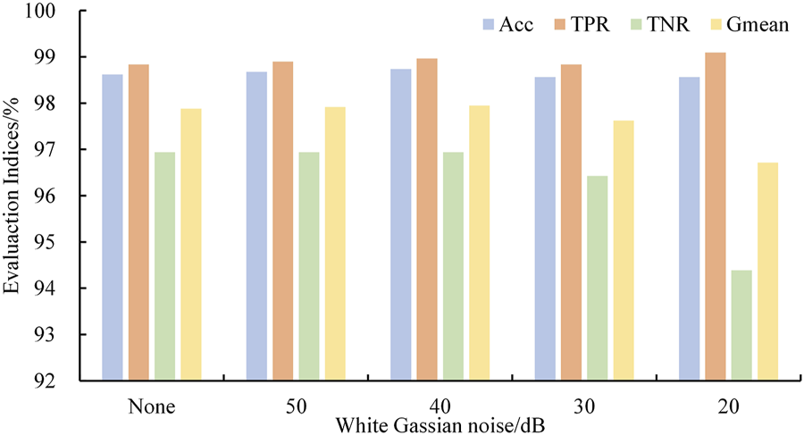
The performance of CasLightGBM considering noise interference.
Conclusion
Taking sample imbalance and overlapping into a comprehensive account, this article developed an FL function rectified CasLightGBM approach for intelligent STVS assessment. The extensive numerical tests are carried out on the IEEE 118-bus system, and the conclusions are drawn as follows:
1) Compared with the dimension of the original feature, the dimension of the key features extracted by mRMR is significantly reduced compared with the dimension of original features, which effectively avoids the problem of dimension explosion.
2) Aided by the FL function, CasLightGBM pays more attention to unstable samples and difficult-to-classify samples, and the obtained TNR and Gmean are better.
3) Compared to other machine learning methods, CasLightGBM has higher Acc, TPR, TNR, and Gmean, and the anti-noise performance is excellent. This performance enhancement contributed to executing timely emergency control measures for less load shedding amount.
In the actual operation of the power grid, factors such as equipment maintenance and natural disasters will lead to frequent changes in the power grid topology, which poses a huge challenge to the data-driven STVS assessment technology. In relevant future work, how to learn the topology of the power grid will be further analyzed and discussed to make the evaluation model more adaptable in the new topology scenarios.
Statements
Data availability statement
The raw data supporting the conclusion of this article will be made available by the authors, without undue reservation.
Author contributions
RZ is responsible for the methodology and manuscript writing, DW is responsible for the compilation of the algorithm, and ZS is responsible for data processing and supervision. All authors contributed, read, and approved the submitted version.
Funding
This work was supported by the National Natural Science Foundation of China (No. 52167015- Research on regulation of high penetration of renewable energy applied to wind/light energy rich areas in Tibet).
Conflict of interest
DW and ZS were employed by the company State Grid Tibet Electric Power Co., Ltd.
The remaining authors declare that the research was conducted in the absence of any commercial or financial relationships that could be construed as a potential conflict of interest.
Publisher’s note
All claims expressed in this article are solely those of the authors and do not necessarily represent those of their affiliated organizations, or those of the publisher, the editors, and the reviewers. Any product that may be evaluated in this article, or claim that may be made by its manufacturer, is not guaranteed or endorsed by the publisher.
References
1
Dasgupta S. Paramasivam M. Vaidya U. Ajjarapu V. (2013). Real-Time Monitoring of Short-Term Voltage Stability Using PMU Data. IEEE Trans. Power Syst.28 (4), 3702–3711. 10.1109/TPWRS.2013.2258946
2
De La Ree J. Centeno V. Thorp J. S. Phadke A. G. (2010). Synchronized Phasor Measurement Applications in Power Systems. IEEE Trans. Smart Grid1 (1), 20–27. 10.1109/TSG.2010.2044815
3
Diao R. Sun K. Vittal V. O'Keefe R. J. Richardson M. R. Bhatt N. et al (2009). Decision Tree-Based Online Voltage Security Assessment Using PMU Measurements. IEEE Trans. Power Syst.24 (2), 832–839. 10.1109/tpwrs.2009.2016528
4
Dong Y. Xie X. Zhou B. Shi W. Jiang Q. (2016). An Integrated High Side Var-Voltage Control Strategy to Improve Short-Term Voltage Stability of Receiving-End Power Systems. IEEE Trans. Power Syst.31 (3), 2105–2115. 10.1109/TPWRS.2015.2464695
5
Fernandes E. R. Ghiocel S. G. Chow J. H. Ilse D. E. Tran D. D. Zhang Q. et al (2017). Application of a Phasor-Only State Estimator to a Large Power System Using Real PMU Data. IEEE Trans. Power Syst.32 (1), 411–420. 10.1109/TPWRS.2016.2546947
6
Glavic M. Novosel D. Heredia E. Kosterev D. Salazar A. Habibi-Ashrafi F. et al (2012). See it Fast to Keep Calm: Real-Time Voltage Control under Stressed Conditions. IEEE Power Energy Mag.10 (4), 43–55. 10.1109/mpe.2012.2196332
7
He X. Ai Q. Qiu R. C. Huang W. Piao L. Liu H. (2015). A Big Data Architecture Design for Smart Grids Based on Random Matrix Theory. IEEE Trans. Smart Grid8 (2), 1. 10.1109/TSG.2015.2445828
8
Hu X. Zhang H. Ma D. Wang R. (2021). A tnGAN-Based Leak Detection Method for Pipeline Network Considering Incomplete Sensor Data. IEEE Trans. Instrum. Meas.70, 1–10. 10.1109/TIM.2020.3045843
9
Ke G. Meng Q. Finley T. Wang T. Chen W. Ma W. et al (2017). Lightgbm: A Highly Efficient Gradient Boosting Decision Tree. Proc. Adv. Neural Inf. Process. Syst.30, 3146–3154. 10.5555/3294996.3295074
10
Kundur P. Paserba J. Ajjarapu V. Andersson G. Bose A. Canizares C. et al (2004). Definition and Classification of Power System Stability IEEE/CIGRE Joint Task Force on Stability Terms and Definitions. IEEE Trans. Power Syst.19 (3), 1387–1401. 10.1109/TPWRS.2004.825981
11
Li S. Hou J. Yang A. Li J. (2021a). DNN-based Distributed Voltage Stability Online Monitoring Method for Large-Scale Power Grids. Front. Energy Res.9, 625914. 10.3389/fenrg.2021.625914
12
Li Z. Liu H. Zhao J. Bi T. Yang Q. (2021b). Fast Power System Event Identification Using Enhanced LSTM Network with Renewable Energy Integration. IEEE Trans. Power Syst.36 (5), 4492–4502. 10.1109/tpwrs.2021.3064250
13
Lin T. Y. Goyal P. Girshick R. He K. Dollar P. (2020). Focal Loss for Dense Object Detection. IEEE Trans. Pattern Anal. Mach. Intell.42 (2), 318–327. 10.1109/TPAMI.2018.2858826
14
Liu S. Shi R. Zhang T. Tang F. Zhang L. Liu L. et al (2021). An Integrated Scheme for Static Voltage Stability Assessment Based on Correlation Detection and Random Bits Forest. Int. J. Electr. Power & Energy Syst.130, 106898. 10.1016/j.ijepes.2021.106898
15
Luo Y. Lu C. Zhu L. Song J. (2021). Data-Driven Short-Term Voltage Stability Assessment Based on Spatial-Temporal Graph Convolutional Network. Int. J. Electr. Power & Energy Syst.130, 106753. 10.1016/j.ijepes.2020.106753
16
Ma D. Hu X. Zhang H. Sun Q. Xie X. (2021). A Hierarchical Event Detection Method Based on Spectral Theory of Multidimensional Matrix for Power System. IEEE Trans. Syst. Man. Cybern. Syst.51 (4), 2173–2186. 10.1109/TSMC.2019.2931316
17
Peng H. Long F. Ding C. (2005). Feature Selection Based on Mutual Information Criteria of Max-dependency, Max-relevance, and Min-Redundancy. IEEE Trans. Pattern Anal. Mach. Intell.27 (8), 1226–1238. 10.1109/TPAMI.2005.159
18
Ren C. Xu Y. Zhang Y. Zhang R. (2020). A Hybrid Randomized Learning System for Temporal-Adaptive Voltage Stability Assessment of Power Systems. IEEE Trans. Ind. Inf.16 (6), 3672–3684. 10.1109/TII.2019.2940098
19
Rizvi S. M. H. Sadanandan S. K. Srivastava A. K. (2021). Data-Driven Short-Term Voltage Stability Assessment Using Convolutional Neural Networks Considering Data Anomalies and Localization. IEEE Access9, 128345–128358. 10.1109/ACCESS.2021.3107248
20
Vanfretti L. Arava V. S. N. (2020). Decision Tree-Based Classification of Multiple Operating Conditions for Power System Voltage Stability Assessment. Int. J. Electr. Power & Energy Syst.123, 106251. 10.1016/j.ijepes.2020.106251
21
Vournas C. D. Nikolaidis V. C. Tassoulis A. A. (2006). Postmortem Analysis and Data Validation in the Wake of the 2004 Athens Blackout. IEEE Trans. Power Syst.21 (3), 1331–1339. 10.1109/TPWRS.2006.879252
22
Yan R. Masood N. A. Kumar Saha T. Bai F. Gu H. (2018). The Anatomy of the 2016 South Australia Blackout: A Catastrophic Event in a High Renewable Network. IEEE Trans. Power Syst.33 (5), 5374–5388. 10.1109/tpwrs.2018.2820150
23
Yang H. C. Qiu R. Tong H. (2020). Reconstruction Residuals Based Long-Term Voltage Stability Assessment Using Autoencoders. J. Mod. Power Syst. Clean. Energy8 (6), 1092–1103. 10.35833/MPCE.2020.000526
24
Yang H. Zhang W. Chen J. Wang L. (2018). PMU-based Voltage Stability Prediction Using Least Square Support Vector Machine with Online Learning. Electr. Power Syst. Res.160, 234–242. 10.1016/j.epsr.2018.02.018
25
Zhang M. Li J. Li Y. Xu R. (2021). Deep Learning for Short-Term Voltage Stability Assessment of Power Systems. IEEE Access9, 29711–29718. 10.1109/ACCESS.2021.3057659
26
Zhang Y. Xu Y. Dong Z. Y. Zhang P. (2019a). Real-Time Assessment of Fault-Induced Delayed Voltage Recovery: A Probabilistic Self-Adaptive Data-Driven Method. IEEE Trans. Smart Grid10 (3), 2485–2494. 10.1109/tsg.2018.2800711
27
Zhang Y. Xu Y. Dong Z. Y. Zhang R. (2019b). A Hierarchical Self-Adaptive Data-Analytics Method for Real-Time Power System Short-Term Voltage Stability Assessment. IEEE Trans. Ind. Inf.15 (1), 74–84. 10.1109/tii.2018.2829818
28
Zhang Y. Xu Y. Zhang R. Dong Z. Y. (2019c). A Missing-Data Tolerant Method for Data-Driven Short-Term Voltage Stability Assessment of Power Systems. IEEE Trans. Smart Grid10 (5), 5663–5674. 10.1109/TSG.2018.2889788
29
Zhong Z. Guan L. Su Y. Yu J. Huang J. Guo M. (2022). A Method of Multivariate Short-Term Voltage Stability Assessment Based on Heterogeneous Graph Attention Deep Network. Int. J. Electr. Power & Energy Syst.136, 107648. 10.1016/j.ijepes.2021.107648
30
Zhou Z.-H. Feng J. (2017). Deep Forest: Towards an Alternative to Deep Neural Networks. Proc. Int. Jt. Conf. Artif. Intell.2017, 3553–3559. 10.24963/ijcai.2017/497
31
Zhu L. Hill D. J. Lu C. (2021). Intelligent Short-Term Voltage Stability Assessment via Spatial Attention Rectified RNN Learning. IEEE Trans. Ind. Inf.17 (10), 7005–7016. 10.1109/TII.2020.3041300
32
Zhu L. Lu C. Kamwa I. Zeng H. (2020). Spatial-Temporal Feature Learning in Smart Grids: A Case Study on Short-Term Voltage Stability Assessment. IEEE Trans. Ind. Inf.16 (3), 1470–1482. 10.1109/tii.2018.2873605
33
Zhu L. Lu C. Liu Y. Wu W. Hong C. (2017). Wordbook‐based Light‐duty Time Series Learning Machine for Short‐term Voltage Stability Assessment. IET Gener. Transm. & Distrib.11 (18), 4492–4499. 10.1049/iet-gtd.2016.2074
Summary
Keywords
data-driven, sample imbalance, cascaded LightGBM, focal loss, short-term voltage stability assessment
Citation
Zhu R, Wang D and Su Z (2022) Data-Driven Short-Term Voltage Stability Assessment Considering Sample Imbalance and Overlapping. Front. Energy Res. 10:902861. doi: 10.3389/fenrg.2022.902861
Received
23 March 2022
Accepted
15 June 2022
Published
15 July 2022
Volume
10 - 2022
Edited by
Chengzong Pang, Wichita State University, United States
Reviewed by
Rui Wang, Northeastern University, China
Dazhong Ma, Northeastern University, China
Updates
Copyright
© 2022 Zhu, Wang and Su.
This is an open-access article distributed under the terms of the Creative Commons Attribution License (CC BY). The use, distribution or reproduction in other forums is permitted, provided the original author(s) and the copyright owner(s) are credited and that the original publication in this journal is cited, in accordance with accepted academic practice. No use, distribution or reproduction is permitted which does not comply with these terms.
*Correspondence: Ruijin Zhu, zhuruijin@xza.edu.cn
This article was submitted to Smart Grids, a section of the journal Frontiers in Energy Research
Disclaimer
All claims expressed in this article are solely those of the authors and do not necessarily represent those of their affiliated organizations, or those of the publisher, the editors and the reviewers. Any product that may be evaluated in this article or claim that may be made by its manufacturer is not guaranteed or endorsed by the publisher.