Marine Biofuels Costs and Emissions Study for the European Supply Chain Till 2030

The design and preliminary estimations of biomass supply chains are essential in matching energy supply to energy demand. This is especially true of novel/future fuels and technologies in large industries. In this paper, a Mixed Integer Linear Programming (MILP) model was formulated to represent biofuel supply chains across Europe for the production of three novel marine fuels and to allow the selection of fuel conversion technologies, biomass supply locations, and the logistics of transportation from resources to conversion and from conversion to final markets. On top of this, the total production costs and emissions were calculated and compared to current marine fuels to assess the implementation potential and feasibility of these fuels. The MILP model was used to design and analyze optimal distribution and conversion systems, using a realistic data-set covering the European member states and 15 of the largest bunkering ports in the EU. The results showed that on average, the fuels obtained a 72% greenhouse gas (GHG) reduction compared to a fossil fuel comparator and ranged from 22–36 €/GJ in total production costs. It was also discovered that forestry residues were the best-suited biomass for the production of these fuels and that Poland had the highest supply potential of all considered states. The available supply of biomass was sufficient for the demand in the foreseeable future, the largest impediment to the adoption of these fuels is the available refining potential in Europe.

1 Introduction

The maritime industry has long relied on oils and heavy fuels as main energy carriers. Though one of the most efficient modes of transport (in terms of costs and emissions per tonne mile), the shipping sector still accounts for an important 2.5% of global greenhouse gas emissions (European Commission, 2016). On top of this, current industry fuels have high levels of sulfur and release nitrogen oxides upon combustion, which both can be extremely harmful to local environments and ecosystems. The largest body in marine regulation; The International Maritime Organization (IMO) has set a goal in reducing total industry emissions to 50% relative to 2008 levels (IMO, 2019). Additionally, the European Union has passed a series of regulations and targets relating to shipping, and there are growing concerns (for ship owners) on the expansion of Emission Control Areas (ECAs) across Europe. However, most of the regulations passed are not yet binding and it is not entirely clear how these goals are to be accomplished.

One of the most promising current solutions to this problem is the use of biofuels. These sustainably-sourced combustibles can cut back total emissions by considerable amounts and are supportable in the medium to long term.

Previous studies for the maritime industry have largely focused on drop-in biofuels based on oily feedstocks. However, recent amendments to regulations (RED II) have outlined various oil-based feedstocks as posing high Indirect Land Use Change (ILUC) and therefore current studies have shifted away from these (EC, 2018). A study carried out by shipping line A.P. Moller—Maersk and classification society Lloyds Register said that based on market projections, the best positioned fuels for research and development into net zero emissions for shipping include alcohols (ethanol and methanol) and biomethane (biofuels news, 2019). This study explores the suitability in terms of production and distribution from cradle-to-gate of these three fuels. The feedstocks as well as the conversion processes considered in this report are displayed in Tables 1, 2.

TABLE 1

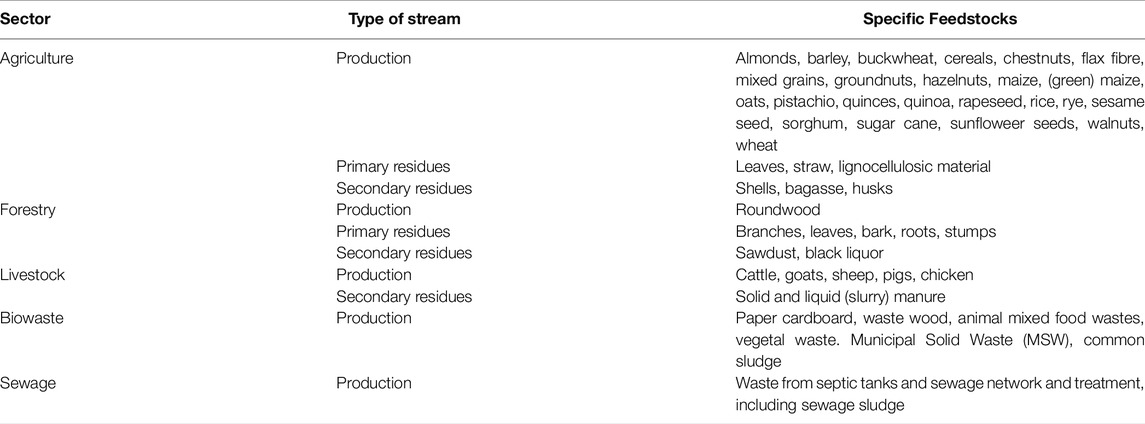
TABLE 1. Specific feedstocks considered, the production stream they fall into and the respective sector. For agriculture, forestry and livestock, only the primary and secondary residues of the product are considered as feedstocks.

TABLE 2

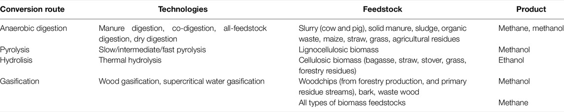
TABLE 2. Conversion type, technologies and end products from considered biomass.

Although in time new refineries can be constructed, in the short run potential supply is fixed and competes with interests from other industries. Therefore, the study is carried out or the period 2025–2030, as the greatest difficulty to cope with demand increase is expected in the early periods, when no additional capacity can be found (van der Kroft, 2020). With Europe leading the way in the shift to low impact fuels, a total of 27 countries are considered in this study; the European member states plus the United Kingdom, Norway and Switzerland. Small countries as Cyprus, Luxembourg and Malta are disregarded in the analysis for now. Additionally the ports considered for the fuel demand are the top 15 most frequented ports across the EU.

It is widely known that the EU’s energy policies head towards the development of renewable energies, seeking to reach energy sustainability by reducing international energy dependence. Though many countries are part of a global/collective effort to combat climate change, the majority of binding policies relating to energy supply and demand are set and enforced at a national level resulting in a divergence between the scope and policy ambitions of separate countries. An economically efficient development of sustainable energy cannot be achieved by Member states alone. The European Union has the necessary policies, funds, cooperation and ambitions to become one of the first areas globally to embark on the journey to the large-scale development of biofuels. Moreover, a coordinated approach avoids fragmentation of goals and is more efficient by fully exploiting economies of scale and technological cooperation.

2 Literature Review

As of today, the most widely used fuels for maritime are Heavy Fuel Oil (HFO) followed by Marine Diesel Oil (MDO) and Liquefied Natural Gas (LNG). There are also certain low-sulfur fuels such as Very Low Sulphur Oil (VLSFO) and Ultra Low Sulphur Oil (ULSFO) that comply with Emission Control Area (ECA) regulations, but these come at the cost of increased prices through extra refining and consequently, higher CO₂ emissions. Since LNG-powered engines exist on a small portion of the fleet, the change to bio-LNG would be relatively simple for these vessels as it does not require any engine retrofitting or new installments (on the ship itself). Insofar as biofuels, present use is centered around oily, drop-in fuels such as biodiesel and hydro-treated vegetable oil. However, in the European Union, the Renewable Energy Directive (RED) II has classified palm oil-based biodiesel under a high Indirect Land Use Change risk category (European Parliment and Council, 2018). As a result, biodiesel consumption in the European Union is expected to fall below current levels.

Biofuel supply chains are often compared to petroleum supply chains, especially in the downstream component (after the fuel conversion). However, the upstream components are very different. Further, the majority of literature on biofuel supply chains is usually focused around the optimization of one fuel in a small area (nationwide). For example, Moretti et al. developed a general modelling approach with a network structure comprising of two intermediate echelons (storage and conversion facilities). Their model accounted for both train and truck freight transport in the production of green methanol in Italy (Moretti et al., 2021). In another example, Ranisau et al. looked into biofuel production from corn stover in Ontario. The superstructure of their model only included three echelons, namely biomass production, conversion and the demand sites. Both of these studies failed to incorporate additional steps in the refining process such as storage and pretreatment. Further, the geographical area considered in these studies was of narrow scope and fit into the same geopolitical assumptions/conditions. Few literature exists on large-scale supply chains for multiple fuels. Therefore, an aspect that calls for more attention in future modelling is the emphasis on the upstream component. A study by van der Kroft at al. delved into the modelling of worldwide biofuel supply chains (van der Kroft, 2020). Unlike most, van der Kroft put emphasis on the down-stream component of the supply chain and included shipping as a form of energy transport between countries.

Traditionally, BSCs are represented through mathematical programming models. The majority fall into two classifications; deterministic or stochastic. In deterministic models, the input parameters are know and fixed with certainty. On the other hand, stochastic models have elements of randomness. Though stochastic models are useful in modelling inherent unknowns and future behaviors, their use implies knowing a variable’s probability distribution, which can be very time and capital consuming.

Within the modelling frameworks, the problem can be solved through both linear and non-linear formulations, though linear is more common. Usually, in literature the measure(s) to be optimized is either some type of costs or emissions, but through a multiple objective formulation can include both and/or others. When using a multi-objective optimization, however, the optimal solution is not at a single point but instead a set of Pareto-optimal solutions. In this set, it becomes impossible to improve any objective without worsening the other. Any point outside this set is either infeasible due to the constraints or sub-optimal.

Within the deterministic formulation of a biofuel supply chain, a MILP is most often used (Kim et al., 2011; Andersen et al., 2012) and MILNP (Zamboni et al., 2009). Recent studies in this field have brought novelty to the optimization process either by considering specific supply chain structures or presenting new solution methods. For example, Lopez Diaz proposed a MINLP model for the design of a bio-refining system in Mexico (Lopez-Diaz et al., 2018). Particular to his model, Lopez modelled the three segments of the supply chain, including the cultivation of the crops and linking it to water use. This is seldom done in literature, as the majority of published works only consider the products when they are ready to be harvested. In another example, Castillo-Villar developed a two stage linear stochastic programming model to minimize costs related to transportation, location, technology and quality with a case study in the state of Tennessee (Aboytes-Ojeda et al., 2019). The stochastic parameters included ash and moisture contents. This was relatively novel, as few studies focus on variability.

Although a large number of contributions are available in the field of biofuel supply chain modelling, there is still room for further investigation. Particularly for maritime fuels, mathematical models addressing the BSC are scarce. Based on the analyzed literature and the current trends in literature, the following research gaps claim for deeper attention:

• The BSC using multiple feedstocks and end products, considering the medium-to-long term supply particularities of the raw materials.

• More in depth attention and modelling of the upstream component of the processing.

• Robust optimization and a higher level of detail with regards to the input data for data modelling.

• A connection/mathematical relationship between the supply and demand. Most models make use of existing data and assumptions to consider the supply and demand aspects separately, while in reality they depend on each other and are tied together through a sort of feedback loop.

In order to address the aforementioned gaps, this study develops a Multi-Objective MILP model to design and optimize the supply chains of bio-ethanol, bio-methanol and bio-LNG from multiple feedstock sources, projecting strategic supply chain decisions in the medium term. The main contributions of the present study lie within the novel fuels being looked at, the robustness of the framework developed, the focus on the upstream supply-chain segments, the lengthy time-frame in question, and the built-in open choice of fuel production.

3 Methodology Overview

In energy systems, conversion technologies are used to transform primary energies into useful carriers. Several technologies may be used simultaneously or in competition using different feedstocks and fuels. The objective is to match the energy requirements at the minimum costs and emissions. In this work, a multi-objective optimization technique is employed to optimize the supply chains of marine biofuels in Europe and to gain insight into the preferred biomass/fuel choices under different scenarios.

The proposed problem can be formulated mathematically as a transhipment problem. In this set up, the network nodes have both input and output simultaneously, with additional supply and demand (origin and destination) points (see Figure 1).

FIGURE 1

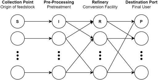
FIGURE 1. Visual representation of supply chain superstructure.

The superstructure of the model itself consists of four echelons, each with their respective nodes. The first echelon, the collection point, consists of 27 nodes (one for each considered country) which have a certain supply of each type of considered biomass for each year in question. The biomass is collected at a specific point in a country and transported in its raw state to a preprocessing facility within the same country. At the pre-treatment plant, all biomass types go through a physical conversion and are densified to remove nearly all moisture content. Once this is done, the pre-treated product is ready for transport. From the country, the biomass travels to a nearby conversion facility where it is converted into one of the three fuels. In this study, it is assumed that biofuel conversion and upgrading are conducted in the same facility. Therefore, the product that leaves the conversion plant requires no further processing. Since the conversion facilities are also the ports (demand sites), once the fuel has been produced, it can either stay at the same port (and contribute to the fuel demand quota at that same port), or be transported by a tanker vessel to another port to meet its demand quota.

Two mathematical functions are proposed in accordance with the sustainability approach; namely, an economic objective which aims for the reduction of total system costs and an environmental, in the reduction of total system emissions.

3.1 Economic Objective Function

The total system costs (C) are the sum of all costs across every time period. As expressed, the total system costs in each time period are divided into the five different costs associated at each phase (Feedstock-FS, Collection-Coll, Pretreatment-Pre, Conversion-Conv and Transport-Trans) in the supply chain plus the deficit cost (Deficit). Each cost is dependent on at least one of the four decision variables.

$C_T=\sum _{t\in T}\left(C_t^{FS}+C_t^{Coll}+C_t^{Pre}+C_t^{Conv}+C_t^{Trans}+C_t^{Deficit}\right)(1)$

Starting from the purchasing of the feedstock to the conversion and transportation.

$C_t^{FS}=\sum _{s\in S}\sum _{b\in B}\left(ub{c}_{s,b,t}\cdot B{U}_{s,b,t}\right)\forall t\in T(2)$

Total feedstock costs are measured as the sum of the total amount (UB) of each type of biomass (b) collected at each country (s) multiplied by the respective unit biomass price (ubc) (per biomass type) at each country in each time period (t).

$\begin{array}{c}{C}_t^{Coll}=\sum _{s\in S}\sum _{b\in B}\left(\frac{B{U}_{b,s,t}\cdot \left(w_{s,t}+r{c}_{s,t}+ct{f}_{s,t}\cdot f{c}^{loader}\right)\cdot 10^3}{{\rho }_b^{wet}\cdot LH{V}_b^{wet}\cdot {\beta }_s^{labor}\cdot r}\right)\\ \forall t\in T\end{array}(3)$

The collection costs can be summarized as the product of the total costs per hour (machine rental (rc), wages (w) and fuel cost (ct) times fuel consumption (fc)) multiplied by the total time needed to load all of the biomass (total biomass energy content divided by lower heating value (LHV), density (ρ) and loading rate in m³/h (r). This is all divided by the productivity of labor in each country (β).

$\begin{array}{c}{C}_t^{Pre}=\sum _{s\in S}\sum _{b\in B}B{U}_{s,b,t}\cdot c{e}_{s,t}\cdot \left(\frac{{sec}_b^{drying}}{LH{V}_b^{wet}}+\frac{{\delta }^{drying}\cdot {sec}_b^{milling}}{LH{V}_b^{dry}}\right)\\ \forall t\in T\end{array}(4)$

Costs of pretreatment consist of two parts; drying and milling. The costs associated with these treatments are mainly those relating to electricity costs (ce) times the consumption of each proces (sec) multiplied by the mass (BU) and diveded by the LHV to convert to energy. Since material is lost during both drying and milling, two constants are added to reflect this; δ^drying and δ^milling. Due to the drying being performed before the milling, the amount of biomass that reaches the mills is reduced by the factor δ^drying as can be seen on the right side of Eq. 4. As the costs are based on the mass input δ^milling does not play a role here, it is only used to calculate the final mass at the end of both processes. This is the total efficiency of the pretreatment process which is the product of both pretreatment yields (δ^drying and δ^milling), this is reflected in the constraints of the model.

$C_t^{Conv}=\sum _{i\in I}\sum _{r\in R}\sum _{p\in P}\sum _{f\in F}\left(\frac{uc{c}_{r,i,f,t}\cdot S{F}_{r,p,f,t}}{{\beta }_r^{Rlabour}}\right)\forall t\in T(5)$

Conversion costs are calculated based on the average cost of producing a unit of the product. In other words, the cost (ucc in €/GJ) associated with producing one GJ of product from the given inputs (shipped amount to the refinery (SF)). Values are pulled from literature and averaged to approximate the operational costs of production. Again, the productivity of labor (β) is factored in to account for an additional or fewer amount of work depending on the country (or refinery) in which the process occurs.

Lastly, the transportation costs are described:

$\begin{array}{ll}\hfill & C_t^{Trans}\hfill \\ \hfill & =\sum _{s\in S}\sum _{b\in B}\left(\frac{B{U}_{s,b,t}\cdot d_s^{OPre}\cdot \left(f{c}^{truck}\cdot ct{f}_{s,t}+w_{s,t}^{TD}/as\right)\cdot 10^3}{LH{V}_b^{wet}\cdot {\rho }_b^{wet}\cdot {\omega }^{truck}}\right)\hfill \\ \hfill & +\sum _{s\in S}\sum _{r\in R}\sum _{i\in I}\left(\frac{T{I}_{s,r,i,t}\cdot d_{s,r}^{SR}\cdot \left(f{c}^{truck}\cdot ct{f}_{s,t}+w_{s,t}^{TD}/as\right)\cdot 10^3}{LH{V}_i^{dry}\cdot {\rho }_b^{dry}\cdot {\omega }^{truck}}\right)\hfill \\ \hfill & +\sum _{r\in R}\sum _{p\in P}\sum _{f\in F}\left(\frac{S{F}_{r,p,f,t}\cdot cr\cdot d_{r,p}^{RP}}{LH{V}_f^{fuel}\cdot av\cdot {\omega }^{ship}}\right)\forall t\in T\hfill \end{array}(6)$

The transportation costs are divided into the three legs of transportation. In the first and second segment (the transport of biomass to the pretreatment facility and the transport of the intermediate to the refinery), the respective products (BU, TI) are carried by truck, for which the limiting carrying capacity is volume (ω). Therefore, the total energy content of the used biomass is transformed into total volume and with the carrying capacity and trip distance (d), the total amount of trips/number of trucks needed is calculated (using speed a). The costs of truck transport include the fuel costs as well as the truck driver wage, which is different in each country. The last leg of transport is calculated slightly differently. The costs are based on the daily chartering rate of tanker vessels. This includes operational costs such as crew, fuel and docking fees. In the case of a tanker vessel, the limiting factor in terms of capacity is the weight, therefore the deadweight tonnage is used in ω^ship.

Additionally, another cost term is added to the equation called “Deficit Cost”. In order for the model to allocate fuel to the respective ports and meet the demand while also minimizing costs, it should receive a penalty for failing to do so. In optimization, these variables are called slack variables, and this one serves to ensure that the model is inclined towards coming as close as possible to the demand even when there is not enough supply. This variable is also present in the constraints, and without it, in cases where the demand is greater than the supply, the model would be unsolvable and be rendered infeasible.

$C_t^{Deficit}=D{T}_{p,t}\cdot c{p}_t(7)$

The deficit cost consists of the decision variable DT_p,t which is the total amount of energy deficit at each port and time period. The cost associated with the energy deficit, cp_t, is the cost of replacing that energy with another clean fuel such as biodiesel or LNG. The value of cp_t is not fixed and will need to be altered for each demand case to a level where the model reaches full demand satisfaction. It is also important to note that although $C_t^{Deficit}$ is included in the total cost function for the optimization, it is not considered in the post-processing values of the cost.

3.2 Environmental Objective Function

The environmental impact of the supply chain is assessed on the basis of total greenhouse emissions released during the 5-year period. This includes all pollutants that can be associated under a CO₂ equivalence indicator. NO_x and SO_x emissions resulting from production and distribution activities will not be accounted for in this calculation, as they are not greenhouse gasses, and therefore cannot be associated under a common indicator.Throughout the emission calculations and for each part, an effort is made to stay within the LCA accounting rules of the RED II, though deviations sometimes have to be made from the guidelines (lack of specific data). For the considered feedstocks, annualized emissions from carbon stock changes caused by land use change are not accounted for in the calculations, as all biomass in question originate as biproducts and thus do not cause ILUC. Further, any emission savings from soil carbon accumulation, CO₂ capture and geological storage and CO₂ capture and replacement as expressed in RED II are not considered. Accounting for these emission factors is difficult and uncertain. Including them could lead to highly optimistic results, thus they have been excluded from the analysis. The effect of this decision on the final result will be a slight overestimation of total emissions (according to the RED II emission calculation rules). Further, emissions from the manufacturing of machinery are not taken into account. In other words, the focus is on operations, as they constitute the bulk of emissions over the long-term.

The total emissions (E) in the system:

$E^T=\sum _{t\in T}\left(E_t^{Coll}+E_t^{Proc}+E_t^{Trans}\right)\forall t\in T(8)$

Compared to the total cost function, there are two main differences in the calculation. First and most apparent, the lack of feedstock emissions, which was already explained. Secondly, the pretreatment and conversion phases are grouped into one stage and are called emissions from processing, E^Proc. This is done in order to be able to use the RED II values as a reference when finding/calculating the total emissions related to the pretreatment and conversion of the biomass.

The emissions related to the biomass collection are proportional to the amount of fuel burned (and the emission factor of diesel (ef)) during the loading process.

$E_t^{Coll}=\sum _{s\in S}\sum _{b\in B}\left(\frac{B{U}_{s,b,t}\cdot f{c}^{loader}\cdot eff\cdot 10^3}{LH{V}_b^{wet}\cdot {\rho }_b^{wet}\cdot r}\right)\forall t\in T(9)$

The processing emissions (upe) are specific to the type of input biomass and fuel output (f) as well as the refinery (r)

$E_t^{Proc}=\sum _{r\in R}\sum _{p\in P}\sum _{b\in B}\sum _{f\in F}S{F}_{r,p,f,t}\cdot up{e}_{b,f}\forall t\in T(10)$

Lastly, the transport emissions are set up similarly to the transportation costs. The emissions at each leg are related to the distance travelled, number of trips (or number of trucks/ships needed to transport all of the product in consideration) and the emission factor of the fuel being used.

$\begin{array}{ll}\hfill E_t^{Trans}& =\sum _{s\in S}\sum _{b\in B}\left(\frac{B{U}_{s,b,t}\cdot d_s^{OPre}\cdot f{c}^{truck}\cdot eff\cdot 10^3}{LH{V}_b^{wet}\cdot {\rho }_b^{wet}\cdot {\omega }^{truck}}\right)\hfill \\ \hfill & +\sum _{s\in S}\sum _{r\in R}\sum _{i\in I}\left(\frac{T{I}_{s,r,i,t}\cdot d_{s,r}^{SR}\cdot f{c}^{truck}\cdot eff\cdot 10^3}{LH{V}_i^{dry}\cdot {\rho }_b^{dry}\cdot {\omega }^{truck}}\right)\hfill \\ \hfill & +\sum _{r\in R}\sum _{f\in F}\sum _{p\in P}\left(\frac{S{F}_{r,p,f,t}\cdot d_{r,p}^{RP}\cdot ef{f}^{ship}}{LH{V}_f^{fuel}}\right)\forall t\in T\hfill \end{array}(11)$

4 Constraints

With the objectives defined and mathematically expressed, the solution should be constrained to reflect the constraints and limitations of reality. A series of equations will be developed to make sure this is the case.

4.1 Non-Negativity Constraints

The first constraints are the non-negativity constraints. These ensure that all decision variables take on positive values, otherwise the system would minimize the objective functions by allowing the largest negative decision variables, which would yield infinitely low emissions and costs. The lower bound on all decision variables is zero. (Φ) is a binary for the selection of which pretreated biomass (i) to convert into which fuel (f) at each refinery (r) and time (t).

$B{U}_{b,s,t}\ge 0\forall b\in B,s\in S,t\in T(12)$

$T{I}_{i,s,r,t}\ge 0\forall i\in I,s\in S,r\in R,t\in T(13)$

$S{F}_{r,p,f,t}\ge 0\forall r\in R,f\in F,p\in P,t\in T(14)$

$D{T}_{p,t}\ge 0\forall p\in P,t\in T(15)$

${\mathrm{\Phi }}_{r,i,f,t}\ge 0\forall r\in R,i\in I,f\in F,t\in T(16)$

4.2 Capacity Constraints

Each biorefinery has a certain capacity of fuel production for each type of fuel. For this to be reflected in the model, a capacity constraints should be made for each refinery (rcap is this capacity). The same goes for the ports. However, it is assumed that ports have unlimited storage capacity when it comes to these three fuels. In reality, a real representation of port LNG capacity can be obtained. Port-specific capacity data for methanol and ethanol however, is not available due to the novelty and lack of current use. Regardless, port capacities for the considered fuels are assumed to be unlimited. This way the fuels will flow to the most economic/least environmentally harmful ports without the constraints of present-day infrastructure, which will be useful for the determination of future infrastructure investments. The following constraint ensures that the maximum fuel production level for each fuel and refinery during every time period is maintained at all times.

$\sum _{p\in P}S{F}_{r,p,f,t}\le rca{p}_{r,f,t}\forall p\in P,f\in F,t\in T(17)$

4.3 Energy Balance Constraints

To ensure that the same amount of product (in terms of energy and including losses and efficiencies) flows through the nodes, energy balancing constraints should be placed at each node. To start, the amount of biomass collected should be equal to the amount of intermediate product trucked for each type of biomass and from each country.

$\begin{array}{c}\sum _{b\in B}\left(B{U}_{s,b,t}\cdot {\delta }^{drying}\cdot {\delta }^{milling}\right)-\sum _{r\in R}\sum _{i\in I}T{I}_{s,r,i,t}=0\\ \forall t\in T,s\in S\end{array}(18)$

The amount of intermediate product being transported to the refineries should also be equal to the amount of fuel leaving the refineries, accounting for the conversion yield, and efficiencies. ${\delta }_{i,f}^{con}$ represents the yield of converting the intermediate product into a biofuel.

$\begin{array}{c}\sum _{i\in I}\sum _{s\in S}\left(T{I}_{s,r,i,t}\cdot {\delta }_{i,f}^{con}\cdot {\mathrm{\Phi }}_{r,i,f,t}\right)-\sum _{p\in P}S{F}_{r,p,f,t}=0\\ \forall f\in F,t\in T,r\in R\end{array}(19)$

Since some feedstocks have multiple conversion pathways and can be converted into different fuels, a constraint is needed to allow for the selection, but also to prevent double (or triple counting).

$\sum _{f\in F}{\mathrm{\Phi }}_{r,i,f,t}=1(20)$

That is, each inflow of a certain type of biomass from any country at any refinery can only be turned into one type of fuel (otherwise the model would turn it in two all three, which would go against the laws of physics).

4.4 Supply and Demand Constraints

The demand constraint ensures that the total demand for each biofuel type at each port is met by the conversion facilities and the transport network. However, the production of a surplus in line with fuel availability is allowed. The purpose of this constraint is to ensure that at least each port is met with the suffice amount of fuel. The slack variable DT_p,t is present again here to allow for a deficit when needed.

$D{F}_{p,t}-D{T}_{p,t}\le \sum _{r\in R}\sum _{f\in F}S{F}_{r,p,f,t}\forall p\in P,t\in T(21)$

For the supply, the total amount of used biomass of type b in country s during time period t should not exceed the available supply. The following equation ensures this.

$S{B}_{s,b,t}\ge B{U}_{s,b,t}\forall s\in S,b\in B,t\in T(22)$

The model was programmed in Python and Gurobi was used to solve the MILP model.

5 Supply and Demand

Before the available and required energies can be matched, it is necessary to outline the biomass supply, energy demand, and the available facilities for refining and conversion.

5.1 Biomass Supply

For the future supply prediction of the different biomasses, three separate scenarios are developed to encapsulate the inherent uncertainty faced when modelling future conditions. Starting with a baseline scenario based on current/past data and a continuation of historical trends, the supply is also looked at from both high and low availability scenarios. The main difference in the calculation of the three schemes lies in the assumed future biomass competition and specific industry growth.

The baseline availability of each biomass type is calculated in a separate way depending on the available data. For homegenity sake, the data collected is taken primarily from Eurostat () and FAOSTAT (). The maritime industry will face direct competition from other industries for the procurement and utilization of the available biomass. In order to capture this competition, data on current industry energy use will be compiled and compared using an energy balance. The main sources of competition and final end users of renewables include the industry sector, the transport sector and commercial and public services. Current biofuel and energy production is centered around first generation biomass, and will slowly shift to second generation sources over time. Third and fourth generation biomass sources could change near future biomass competition and use depending on their rate of development and adoption. The data of the baseline (current demand and growth) was taken as the basis. In the high competition scenario, the growth of demand was doubled, while in the low competition scenario the growth was the negative of the current growth.

To start, the amount of agricultural residues potentially available for bioenergy production is calculated as the difference between the total produced residues (total amount of crop produced times the residue-to-crop ratio) and the sum of residues left on the field and those used for other purposes. In a similar way, forestry residues are the sum of the total woodchips produced from forestry activities and the recoverable wood products from wood processing. Animal wastes are calculated on the basis of total livestock heads for each animal type per country, the average daily manure production of each animal, and the manure’s moisture content. Organic and biowaste potentials are taken as the recoverable fraction of the total amount produced in the in-scope countries (see Figure 2).

FIGURE 2

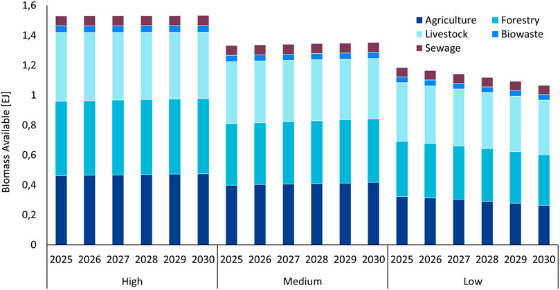
FIGURE 2. Biomass supply scenarios.

Additional to the supply of biomass, the distribution of biofuel refineries across Europe is needed. Based on data from Concawe (ESER, 2021), the locations along with the respective capacities and type of fuel produced are mapped out. These are presented in Table 3.

TABLE 3

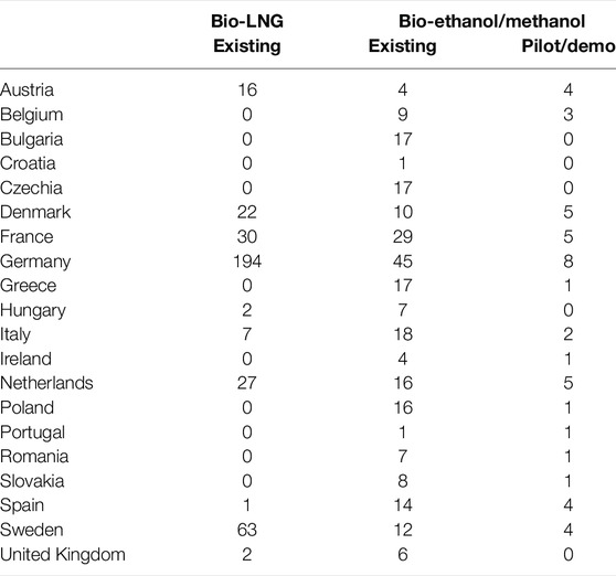
TABLE 3. Overview of currently existing biomass refineries in Europe.

The refineries are classified into two primary groups; Bio-LNG and Bio-Liquid (ethanol and methanol, but also others) facilities. The bio-LNG refineries are well documented and straightforward. Data on other bio-refineries, especially the type and outputted product, is more difficult to assess. Different sources show different numbers for different types of refineries. In order to tackle this, the total amount of bio-liquid refineries are calculated in each country and are multiplied by the proportion of output capacity of a certain bio-liquid to total bio-liquid output in Europe. This can be though of as an averaging technique. This figure is multiplied by the average output of a medium sized refinery (specific to each fuel and feedstock). Further, the pilot plants under construction are considered for expansion of capacities in the coming years. The refineries are then grouped and their capacities are assigned to the closest port. In other words, the refineries are assumed to be at the ports and the total outputting capacity of a port is proportionate to the capacities of the refineries in its vicinity.

5.2 Biomass Demand

In the case of the biofuels in general (bio-LNG, bio-ethanol, bio-methanol and others) in the marine industry, the main two initiatives for the pursuit of environmentally-friendly innovation are operational drivers in the form of cost reduction and regulatory policy (Aronietis et al., 2016). Detailed demand per fuel is not available, hence this section focusses on the general demand.

The general trend of rising oil prices in combination with the volatility of the market has created a market of new fuels to dampen the effects of crude-oil price uncertainty (Ciria and Barro, 2016). Assessing and comparing the costs of advanced biofuels is an objective of this report, however, current and future regulations are unresolved and not binding. The current imposed European mandate from RED II sets the goal of having at least 40% of the EU’s gross final energy consumption be renewable by 2030. However, the RED II also outlines a separate sub-target that relates to transport, although it does not mention the maritime sector. Within the 14% transport sub-target, there is a dedicated target for advanced biofuels produced from feedstocks listed in Part A of Annex IX. The contribution of advanced biofuels and biogas produced from the feedstock listed in Part A of Annex IX as a share of final consumption of energy in the transport sector shall be at least 0.2% in 2022, at least 1% in 2025 and at least 3.5% in 2030 (see also Table 4). As the fuels considered in this report are considered advanced, the targets used for the future demand are these.

TABLE 4

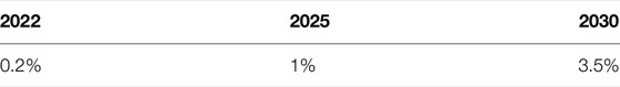
TABLE 4. Share of advanced biofuel targets as a percentage of total energy use according to RED II.

In order to convert this percentage into an amount of energy, the total current and predicted consumed energy in the maritime sector should be calculated. It is assumed that each energy sector complies with the above target and thus only the bunkering energy is relevant for the maritime industry.

Total marine bunker fuel demand is considered in the IEA’s World Energy Model, the OPEC World Energy Model and the EIA’s (Energy Information Administration) World Energy Protection Model at both the collective and regional levels. The IMO also publishes a recurrent study on fleet emissions to gain insight into GHG emissions, fleet development, fuel use and bunker demand. The most recent study, the Fourth IMO GHG study 2020 builds on past developments and uses new data to produce more reliable GHG inventories. It is also the first study to distinguish between international and domestic shipping on a voyage basis (IMO MEPC, 2021). The study identifies two main factors in the transport demand projection, namely, the long-term socio-economic scenarios. GDP and population growth are the two main indicators in this, the higher the predicted growth of these two variables, the higher the projected transport work for products that are positively correlated to them. Second, the long-term energy demand scenario. Higher consumption of fuels leads to higher transport work. To account for different recovery scenarios from corona, GDP growth, population change, etc., the latest IMO report has come up with a set of different scenarios that depict multiple future possibilities of worldwide marine energy demand. Three of those scenarios are used in this report as benchmarks for low, medium and high demand cases.

To assess maritime energy demand in Europe per port, the proportion of fuel consumed at European ports is taken as a fraction of total world consumption. As a rough estimate, the share of bunker energy demand in Europe lies between 20 and 25% of all worldwide bunker energy demand depending on the year in question (IEA, 2020). This figure might seem large, however, a small number of ports account for the majority of the worldwide sales, of which Algeciras, Rotterdam and Antwerp are significant (Lin, 2021).

The OPEC released a World Oil Outlook in 2014 outlining several supply and demand scenarios for the oil industry. In it, key figures were provided on the bunker sales of key worldwide ports (OPEC, 2014). By using a historic approximation of the share of worldwide bunker sales of the main European ports from the IEA 2021 and normalizing them with respect to the total European marine energy demand, one can estimate the percentage of bunker energy demand for each of the in-scope ports (with respect to Europe). Three scenarios are developed based on the IMO GHG scenarios and the RED II advanced biofuel targets. In the high scenario, the RED II targets are taken as twice the nominal values. These scenarios are depicted in Figure 3. For readability, only the top five ports are shown.

FIGURE 3

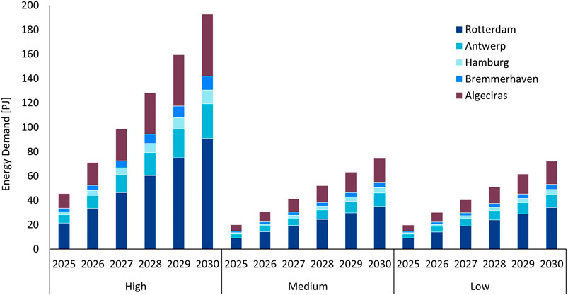
FIGURE 3. Biomass demand scenarios.

6 Results

The developed model was made to determine the optimal sourcing of biomass, the type, product flows and associated supply-chain costs and emissions. From the run scenarios, much information could be gathered.

6.1 Biomass Selection and Fuel Production

To start, one of the most apparent and clear outputs of the model in the various scenarios was the choice of biomass. Unmistakably, the model showed an overall inclination towards forestry residue biomass in every scenario. This choice was due to a balance of biomass physical properties, price and source location. The conversion and transportation advantages of this feedstock proved to outweigh the costs of the biomass and relative transport distance to conversion plants. It was also noted that the option to use forestry residues was more prevalent in scenarios with low or medium demands. When the demand was increased over a certain threshold (around 100 PJ per year, but also depending on the supply scenario), the model ran into an availability constraint with respect to forestry residues and opted for different feedstock choices. For options in which only one specific fuel was used, the choices differed. In the case of ethanol production, forestry residues still reigned supreme. For methanol, agricultural residues and livestock manure also made up a large quantity, and for LNG a significant portion of the feedstock was manure, on top of forestry residues.

The biomass suppliers were rather consistent throughout all run scenarios. The vast majority of biomass energy was supplied from Poland in the form of forestry residues. France was the runner up, followed by the Netherlands, which mainly supplied manure. Romania, Slovenia, Estonia and Spain all supplied a much lower quantity of biomass energy. The rest of the countries supplied biomass to a much lower extent. The countries with the lowest use included Czechia, Finland, Ireland, Sweden, Switzerland and United Kingdom. Factors such as biomass availability, geographical location, proximity to refinery, fuel yield, feedstock prices and available trade routes were all determinants of a specific feedstock uptake. It was discovered that physical properties bore more weight in the selection than originally believed. On top of this, since the pretreatment of biomass was assumed to take place within the country of origin, and the pretreatment cost was largely a function of electricity cost and moisture content as well as LHV, countries with lower electricity costs were more suitable for sourcing. The preferred bio-types were those with low moisture contents and high lower heating values (such as wood), or those that were located relatively close to the refineries (small countries with ports, i.e. Netherlands, Belgium).

In terms of fuel production, the choice to produce one over another turned out to be largely dictated by the available processing capacities. There was a stronger inclination towards ethanol and methanol than LNG, mainly due to the installed capacities of both.

6.2 Trade Routes

The trade routes were also very centered around a few strong ones, given that the biomass sources remained mostly constant in all scenarios. The routes between countries and ports were fairly straightforward, with a propensity towards the shortest path while still meeting refinery capacity constraints. Poland was a main exporter to the two German ports; Bremmerhaven and Hamburg, but also Antwerp and Gdansk. France mainly exported to Le Havre, but also Rotterdam and Antwerp when local capacities were used up. Insofar as the shipping routes, the majority of the product transport was centered around the northern European ports, specifically Rotterdam, Antwerp, Hamburg and Bremmerhaven (See Figure 4). Though the capacities of Bremmerhaven and Hamburg were equal, Hamburg in general had more fuel outflows, since it is located more towards the east, where the majority of biomass originates from. Most of the biofuel produced in Rotterdam remained at Rotterdam to meet the energy demand quota there. In cases where the demand was low however, Rotterdam became a major exporter to all ports (depending on the scenario).

FIGURE 4

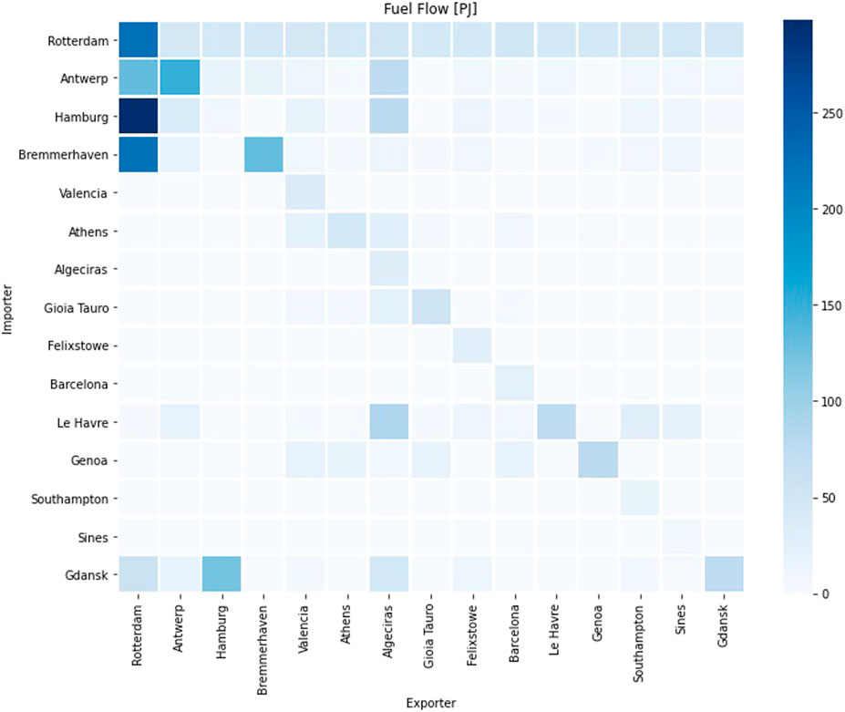
FIGURE 4. Heatmap of total fuel flows from origin port (vertical axis) to destination port (horizontal axis) for base case.

It was also noticed that in times when an energy deficit was necessary (the high demand cases, ethanol, LNG), the largest deficits would generally appear in the southern-Atlantic ports of Algeciras and Sines, as well as Barcelona. Algeciras by far had the largest deficits in terms of total energy. However, as a percentage of local demand, the deficits in Spain and Portugal were quite substantial. Moreover, a very large amount of fuel is shipped to these locations from the northern seaports. It is not the case that Spain and Portugal do not have the necessary supply of biomass, however, there is a strong absence of refining capabilities in those countries. Algeciras would greatly benefit from a larger installment of refineries, and could possibly become a large exporter to the Mediterranean ports if this was the case.

7 Costs and Emissions

Though the emission abatement range was comparably very tight (in terms of what was achievable) for all fuels and cases, the specific costs and emissions were not all that similar. It was found that emission abatement was almost entirely reliant on the conversion process, which was specific to the outputted product. Only 72.2–73.6% of an emission reduction (compared to the fossil fuel comparator; 94 kgCO₂/GJ) was achievable depending on the scenario (See Figure 5). The case of ethanol proved to have the lowest unit energy emissions albeit at the cost of some of the highest unit energy costs. The case of methanol demonstrated both the highest unit emissions and costs, although it was the only fuel out of the three that was able to satisfy the energy demand completely. For this reason, the comparison between the fuels alone is not fully comparable, as with the other two fuels, the cheapest production paths were used up first, resulting in lower specific costs/emissions.

FIGURE 5

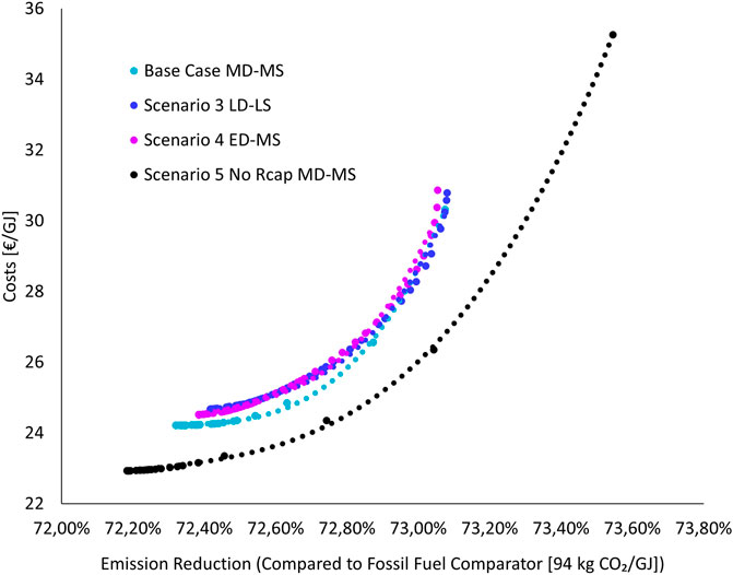
FIGURE 5. Marginal costs of emission abatement.

The average production costs ranged from 22–38 €/GJ and the average emissions from 25–37 kgCO₂/GJ. The costs were mainly distributed over the conversion, pretreatment and to a lesser extent, biomass costs and the second transport leg. The first transport leg costs, collection costs and the shipping costs were found to not be substantial in the whole analysis. To a certain extent, the emission distribution was found to be completely dominated by the conversion process. All other emission components combined did not even account for 10% of the total emissions in any scenario. This can be seen from Figures 6, 7.

FIGURE 6

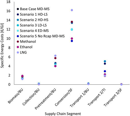
FIGURE 6. Specific energy costs per supply chain segment.

FIGURE 7

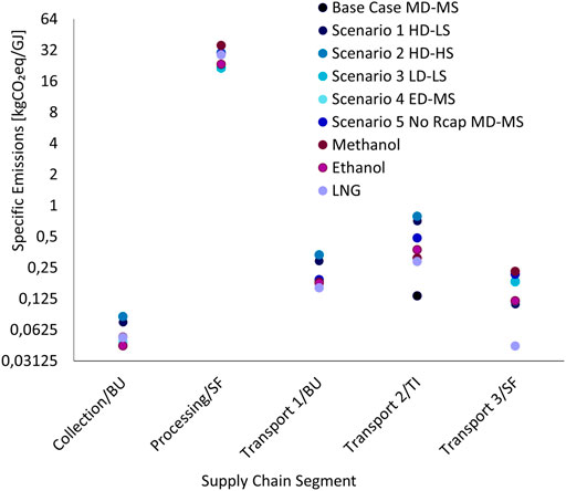
FIGURE 7. Specific emissions per supply chain segment.

8 Conclusion

This study assessed the economic and environmental potential of three new maritime biofuels as well as the feasibility of their adoption within the constraints that were looked at. A MILP model was formulated throught the use of python, GUROBI and an excel database to work out the most optimal flow of goods throughout the supply chain. On top of this, multiple scenarios pertaining to future supply and demand of these biofuels were developed and analyzed within the model to account for future uncertainty. In most scenarios, the European supply of biomass was able to supply around 4% of the top 15 European port’s energy.

With respect to the economic objectives of the model, the difference between these biofuels is still 2–3 times the price of traditional maritime fuels. On average, these clean fuel options will range from 22–25 €/GJ setting them much higher than traditional fuels such as VLSFO, MGO, MDO, LNG, and IFO. However, total supply-chain emissions are cut by around 70%. The question of whether the abatement merits the associated costs is ultimately up to legislators and the objectives of the EU with respect to carbon emissions. Regardless, it can be expected that if this is the case, shipowners would require a subsidy to account for their already tight margins.

Apart from the legislative and logistical barriers to the adoption of these fuels, the biggest obstacle lies within the production capacity (number and output of refineries). The amount of available biomass is more than sufficient to meet the RED II targets in all considered scenarios. Currently, Europe has the capacities to meet the nominal fuel energy demand under medium and low conditions. However, the high supply condition, which considers an energy target of twice the RED II mandate, is unattainable.

In terms of the sourcing and type of biomass, in all scenarios, the majority of the biomass is sourced from Poland in the form of forestry residues. Forestry residues show the highest uptake of all biomass types due to their high energy density (transport-ability), availability and price. A combination of geographical location (proximity to refineries and large ports), low wages, and cheap electricity make Poland the best candidate for the supply of these. However, there is still relatively high biomass uptake in France, Romania and the Netherlands. The countries lacking significant production capabilities include Spain and Portugal, which despite having large amounts of available biomass, rely heavily on the northern seaports for the supply of final energy products.

In conclusion, bio-methanol, bio-ethanol and bio-LNG show promising potentials (insofar as the production logistics and carbon emission reduction) in their use as maritime fuels. Their costs are still much greater than their petroleum counterparts, however, they can offset emissions by up to 73%. Though there is not enough biomass to source the entirefleet with these clean fuels, a small portion (greater than the RED II targets) can be sourced from them. The switch to advanced biofuels will not curb emissions in the maritime sector, however, it could significantly cut back emissions and noxious gasses near ports and heavily frequented European passages for a small portion of the fleet. These fuels present a favorable option for small to mid-sized, short-range vessels.

The present work considers five biomass types (see also Table 1) from public information databases. Additionally, the presented model did not allow for “jumping” over superstructure nodes. Future models should consider expanding the origin sources of the considered biomass, exploring different choices, and including the option for superstructure nodes to be skipped when not necessary (i.e., skip the pretreatment node when not strictly necessary nor beneficial).

Data Availability Statement

The original contributions presented in the study are included in the article/supplementary material, further inquiries can be directed to the corresponding author.

Author Contributions

The research was executed by NG under the Supervision of JP. Similarly the paper was drafted by NG and reviewed and improved by JP.

Funding

This project was partially funded by Nederland Maritiem Land under the MIIP arrangement (MIIIP012 2021 SUSTBIOMASS) as part of the MIIP arrangement for pre-investigations. The publication was made possible by the open access agreement with the TU Delft Library 2021-NN-0007.

Conflict of Interest

The authors declare that the research was conducted in the absence of any commercial or financial relationships that could be construed as a potential conflict of interest.

Publisher’s Note

All claims expressed in this article are solely those of the authors and do not necessarily represent those of their affiliated organizations, or those of the publisher, the editors and the reviewers. Any product that may be evaluated in this article, or claim that may be made by its manufacturer, is not guaranteed or endorsed by the publisher.

References

Aboytes-Ojeda, M., Castillo-Villar, K. K., and Eksioglu, S. D. (2019). Modeling and Optimization of Biomass Quality Variability for Decision Support Systems in Biomass Supply Chains. Ann. Oper. Res. 314 (12). doi:10.1007/s10479-019-03477-8

CrossRef Full Text | Google Scholar

Andersen, F., Iturmendi, F., Espinosa, S., and Diaz, M. S. (2012). Optimal Design and Planning of Biodiesel Supply Chain with Land Competition. Comput. Chem. Eng. 47, 170–182. doi:10.1016/j.compchemeng.2012.06.044

CrossRef Full Text | Google Scholar

Aronietis, R., Sys, C., van Hassel, E., and Vanelslander, T. (2016). Forecasting Port-Level Demand for LNG as a Ship Fuel: the Case of the Port of Antwerp. J. Shipp. Trd. 1, 1–22. doi:10.1186/s41072-016-0007-1

CrossRef Full Text | Google Scholar

biofuels news (2019). Maersk, Lloyds Register Promote Ethanol, Biomethane as Net Zero Fuels for Shipping. Biofuels Int. Mag. Available at: https://biofuels-news.com/news/maersk-lloyds-register-promote-ethanol-biomethane-as-net-zero-fuels-for-shipping/visited 30-06-2022.

Google Scholar

Ciria, P., and Barro, R. (2016). Biomass Resource Assessment. Elsevier, 53–83. doi:10.1016/B978-1-78242-366-9.00003-4

CrossRef Full Text | Google Scholar

EC (2018). Directive (EU) 2018/2001 of the European Parliament and of the Council of 11 December 2018 on the Promotion of the Use of Energy from Renewable Sources. Official J. Eur. Union, 82–328.

Google Scholar

ESER (2021). Refineries Map - Concawe. Available at: https://www.concawe.eu/refineries-map/.

Google Scholar

European Commission (2016). Reducing Emissions from the Shipping Sector - European Commission. Available at: https://ec.europa.eu/clima/policies/transport/shipping_en.

Google Scholar

European Parliment and Council, (2018). EUR-lex - 32018L2001 - EN - EUR-Lex.

Google Scholar

IEA (2021). Oil - Fuels & Technologies - IEA. Available at: https://www.iea.org/fuels-and-technologies/oil.

Google Scholar

IEA (2020). World Energy Outlook 2020 Summary (IEA).

Google Scholar

IMO (2019). IMO’s Work to Cut GHG Emissions from Ships.

Google Scholar

Imo Mepc, (2021). Fourth IMO Greenhouse Gas Study. International Maritime Organization.

Google Scholar

Kim, J., Realff, M. J., Lee, J. H., Whittaker, C., and Furtner, L. (2011). Design of Biomass Processing Network for Biofuel Production Using an MILP Model. Biomass Bioenergy 35, 853–871. doi:10.1016/j.biombioe.2010.11.008

CrossRef Full Text | Google Scholar

Lin, M. (2021). TradeWinds Survey: Main Bunkering Hubs Well Prepared for IMO 2020. TradeWinds.

Google Scholar

López-Díaz, D. C., Lira-Barragán, L. F., Rubio-Castro, E., You, F., and Ponce-Ortega, J. M. (2018). Optimal Design of Water Networks for Shale Gas Hydraulic Fracturing Including Economic and Environmental Criteria. Clean. Techn Environ. Policy 20, 2311–2332. doi:10.1007/s10098-018-1611-6

CrossRef Full Text | Google Scholar

Moretti, L., Milani, M., Lozza, G. G., and Manzolini, G. (2021). A Detailed MILP Formulation for the Optimal Design of Advanced Biofuel Supply Chains. Renew. Energy 171, 159–175. doi:10.1016/j.renene.2021.02.043

CrossRef Full Text | Google Scholar

OPEC (2014). World Oil Outlook 2014.

Google Scholar

van der Kroft, D. (2020). The Potential of Drop-In Biofuels for the Maritime Industry: A MILP Optimization Approach to Explore Future Scenarios. TU Delft.

Google Scholar

Zamboni, A., Bezzo, F., and Shah, N. (2009). Spatially Explicit Static Model for the Strategic Design of Future Bioethanol Production Systems. 2. Multi-Objective Environmental Optimization. Energy fuels. 23, 5134–5143. doi:10.1021/ef9004779

CrossRef Full Text | Google Scholar

Nomenclature

${\mathit{\rho }}_{\mathit{b}}^{\mathit{b}}$ density biomass type b [kg/m³]

${\mathit{\rho }}_{\mathit{i}}^{\mathit{i}}$ density intermediate product type i [kg/m³]

A_s area of country s [km²]

as average speed truck [km/h]

B the five biomass types: MSW, Sewage, Manure, Wood residues, Agricultural Residues

BU_s, b, t amount of biomass b ∈ B from country s ∈ S used during time period t ∈ T

C^Coll total collection costs [€]

C^Conv total conversion costs [€]

ce_s, t cost of electricity in country s during period t [€/GJ]

C^FS total feedstock costs [€]

C^Pre total pretreatment costs [€]

cr chartering rate for specific ship [/h]

ctf_s, t cost of diesel in country s during time period t [€/l]

C^Trans total transportation costs [€]

DF_f, p, t total energy demand in port p during period t [GJ]

d^OPre_s road distance from biomass collection point in country s to pre-treatment in country s [km]

d^RP_r, p navigational distance from refinery r to port p [nm]

d^SR_s, r road distance from country s center to refinery r [km]

DT_p, t fuel energy deficit for port p ∈ P during period t ∈ T

E^Coll total emissions from the collection of raw materials [gCO₂eq]

efbf emission factor of bunker fuel [CO₂eq/l]

eff emission factor diesel [CO₂eq/l]

E^Proc total emissions from processing [gCO₂eq]

E^Trans total emissions from transportation [gCO₂eq]

F fuels: Bio-ethanol, bio-methanol, bio-LNG

fc^loader fuel consumption front loader [l/h]

fc^truck fuel consumption truck [l/h]

I pretreated biomass (same as biomass types but with different physical properties)

LVH^dry_b lower heating value dry biomass b [MJ/kg]

LVH_f lower heating value fuel f [MJ/kg]

LVH^wet_b lower heating value wet biomass b [MJ/kg]

mc_b moisture content for biomass b [%]

P the 15 considered ports for fuel refining and final distribution

R the 15 available integrated refineries across the EU

r volumetric rate of loading for front loader [m³/h]

rcap_r, f refinery production capacity for fuel f at refinery r [GJ]

rc_s, t hourly rental cost of a front loader in country s during period t [/GJ]

S the 27 considered countries of origin for the feedstock

SB_b, s, t supply of biomass b in country s during period t [GJ]

sec^drying_b specific energy consumption of biomass drying [MJ/kg]

sec^milling_b specific energy consumption of biomass milling [MJ/kg]

SF_r, p, f, t shipped amount of biofuel f ∈ F from refinery r ∈ R to port p ∈ P in time period t ∈ T

TI_s, r, i, t transported amount of intermediate product i ∈ B from country s ∈ S to biorefinery r ∈ R in time period t ∈ T

ubc_s, b, t unit biomass cost for biomass b in country s during period t [/GJ]

ucc_r, i, f, t unit conversion costs of producing fuel f from intermediate i in port p during time period t [/GJ]

upe_b, f unit processing emissions for production of fuel f from biomass b [gCO₂eq/GJ]

w_s, t hourly average wage in country s during period t [/h]

w^TD_s, t hourly average truck driver wage in country s during period t [/h]

β^bio_b factor to account for productivity of labor in preprocessing per biomass b [-]

β^labor_s factor to account for productivity of labor per country s [-]

β^Rlabor_r factor to account for productivity of labor in refinery r [-]

δ^con_i, f conversion yield of converting intermediate i into fuel f [%]

δ^drying mass efficiency of drying biomass [%]

δ^milling mass efficiency of milling biomass [%]

Φ_r, i, f, t binary decision variable that selects the conversion of biomass b ∈ B into fuel f ∈ F at refinery r ∈ R during period t ∈ T

ω^ship ship weight fuel capacity [DWT]

ω^truck truck volumetric capacity [m³]