Cation Mixing and Capacity Loss in Li||Ni0.6Mn0.2Co0.2O2 Cells: Experimental Investigation and Application of the Multi-Site, Multi-Reaction Model

We clarify the degradation phenomena in a pouch cell that contains an insertion electrode (Li_zNi_0.6Mn_0.2Co_0.2O₂ or lithated NMC622) and a Li counter electrode. Greater than 500 cycles have been achieved in these cells employing 4 mAh/cm² for both the initial Li metal negative and the NMC622 positive, and we find that cation mixing within the NMC622 is prevalent. That is, transition metals (Ni, and to a lesser extent, Mn and Co) in the transition-metal layer of NMC622 irreversibly exchange places with Li in the Li layer of NMC622, corresponding to a loss of Li sites and a concomitant loss of Coulombic capacity. The use of 1) a perturbation procedure of a recent publication employing the multi-site, multi-reaction model for the porous positive electrode and 2) a procedure to average the degradation phenomena over each cycle, which is shown to be consistent with slow degradation, simplifies the analysis of the experimental data and enables straightforward parameter regression. The resulting agreement between the model calculations and the experimental data is quite good, with the differences being similar to experiment-to-experiment variation.

Introduction

Cells made with Li metal-negative electrodes and lithiated transition metal oxide-positive electrodes are of interest for many applications, including traction batteries. Lithium is the lightest element that is a solid at room temperature, and its high electropositivity (propensity to release its valence electron) yields large cell potentials. In addition, solid Li electrodes have no electrode porosity, binders, conductive diluents, or other characteristics of porous electrodes, making them relatively mass and volume efficient. These considerations help to explain why very high specific energy (Wh/kg) and energy density (Wh/L) can result when Li metal-negative electrodes are employed. The recent perspective article by Liu et al. (2018) underscores these attributes of Li metal batteries, along with a review of continuing challenges. The article by Meibuhr (1970) reviews the early work on Li metal electrodes and non-aqueous electrolytes. In the work of Verbrugge and Koch (1994), electroanalytical studies of the Li-electrolyte interface from the 1970s to the early 1990s are reviewed, with an emphasis on microelectrode investigations, which yield a high signal-to-noise ratio with respect to clarifying interfacial phenomena. Cheng et al. (2017) presented a recent overview of the lithium metal electrode, including working principles and technical challenges. Specific attention is paid to the mechanistic understanding and quantitative models for solid electrolyte interphase [SEI (Peled, 1979; Peled and Menkin, 2017)] formation, and lithium dendrite nucleation and growth. The recent articles by Eijima et al. (2019) and Hobold et al. (2021) provide a review of Li metal electrodes and the influence of various solvents and salts on the formation of the protective SEI and Coulombic efficiency. Chen (2018) provided a rational description of recent work leading to the class of electrolytes we use in this work. Closer to this work in terms of the active materials for the negative and positive electrodes, Xue (2020) investigated Li|| ${\text{Ni}}_{0.6}{\text{Mn}}_{0.2}{\text{Co}}_{0.2}{\text{O}}_2$ cells. They employed a dimethylsulfamoyl fluoride solvent and a lithium bis(fluorosulfonyl)imide salt, which they referred to as a ‘‘full fluorosulfonyl’’ (FFS) electrolyte. Xue (2020) achieved 200 cycles, but it should be noted that their negative/positive ratio was about 8. Niu (2021) also investigated Li|| ${\text{Ni}}_{0.6}{\text{Mn}}_{0.2}{\text{Co}}_{0.2}{\text{O}}_2$ cells. The authors examined the interplay between the negative to positive ratio (n/p) and the initial Li thickness. They employed a lithium bis(fluorosulfonyl)imide salt along with the co-solvents: 1,2-dimethoxyethane and 1,1,2,2-tetrafluoroethyl-2,2,3,3-tetrafluoropropyl ether. They found an n/p ratio of 1 and an initial Li thickness of 20  $\mu$ m to work well, and we take a similar approach in this work.

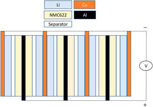
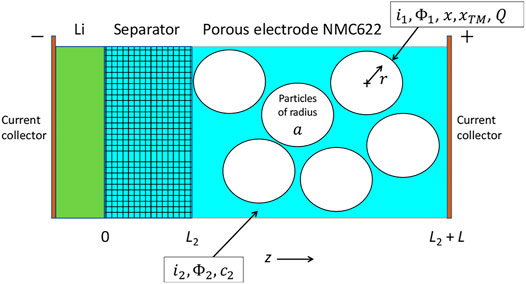
A schematic of the pouch cell employed in this work is provided in Figure 1. Our focus in this work is to model the slow charge of the cell and clarify capacity degradation. We use C/10 charging, where the 1C rate corresponds to the current required to charge a cell from the completely discharged state to the fully, as in fully charged state in 1 h. Because the charge rates are low, as will be shown in the scaling analysis, we can use the perturbation approach recently described in (Baker and Verbrugge, 2021) to treat the data, extract the open-circuit potential of the cell, and clarify degradation, which we find is consistent with cation mixing in the lithiated NMC622 ( ${\text{Li}}_z{\text{Ni}}_{0.6}{\text{Mn}}_{0.2}{\text{Co}}_{0.2}{\text{O}}_2$ , where $0\le z\le 1$ ) positive electrode material (Kim et al., 2016a; Li et al., 2018a; Liao et al., 2005). References to early work on cation mixing in metal oxides can be found in the work of Rossen et al. (1993b), particularly for ${\text{LiCoO}}_2$ , Rossen et al. (1993a) and Ohzuku et al. (1993) for ${\text{LiCoO}}_2$ and ${\text{LiCo}}_{0.5}{\text{Ni}}_{0.5}{\text{O}}_2$ , and Y-Choi et al. (1996) for ${\text{Li}}_{1-\text{δ}}{\text{Co}}_{\text{y}}{\text{Ni}}_{1-\text{y}}{\text{O}}_2$ . The article by Zheng (2019) is focused on cation mixing in ${\text{LiNiO}}_2$ , which is helpful insofar as of the NMC transition metals, it is Ni²⁺ that is most prone to exchanging with Li⁺ irreversibly, although other transition metals do exchange to a lesser degree. In their comprehensive review of Ni-rich NMC, Schipper et al. (2017) consolidated prior literature and stress that in addition to Ni filling Li sites, Mn and Co do as well. In this work, we draw heavily on the review article by Julien et al. (2016) for the model equations we develop in this work for cation mixing (see Eqs 10, 12). In addition to reviewing prior theoretical work on cation mixing in lithiated and layered metal oxides ( ${\text{LiMO}}_2$ , with M referring to a transition metal), Abdellahi et al. (2016) proposed a lattice model based on first principles to understand cation mixing in ${\text{LiMO}}_2$ compounds. Kim et al. (2016b) specifically addressed cation mixing in NMC622, as did Usubelli (2020) in the context of over-lithiation used to recover capacity, and Li et al. (2018b) showed minimal cation mixing (about 2–3%) in their synthesized single-crystal NMC622 investigation. Kim et al. (2016b), in their work, mention “This phenomenon, cation mixing, increases the irreversible capacity and deteriorates the cycleability … it can be considered as the primary factor of capacity fade and voltage decay in lithium ion batteries.”

FIGURE 1

FIGURE 1. Schematic of the pouch cell used to acquire data.

In this work, we show that because the degradation associated with cation mixing is slow, we can average the degradation reaction over each cycle. The perturbation procedure presented in (Baker and Verbrugge, 2021) is used to derive model equations that are simple to implement, which facilitates parameter regression. The remainder of this publication is organized as follows. Following the Experimental section, the mathematical model employed is detailed and the section ends with the perturbation solution, Eq. 69, used to simulate the experimental data. After the Discussion section, a Summary section and Conclusion section is provided.

Experimental

Chemicals and Materials

The electrode fabrication process, including mixing and coating, was carried out in our laboratory. The cathode was fabricated using NMC622 (BASF) with a stable areal capacity of 4.0 mAh/cm² (charge to 4.3 V vs. Li at a 0.1C charge rate). The lithium anode was purchased from Kisco, Japan, with double-side coated 20-μm-thick Li on an 8-μm-thick Cu substrate.

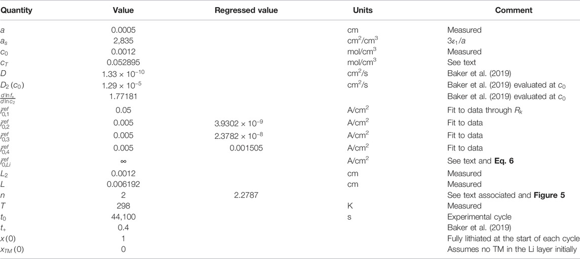
Pouch cells were constructed using a 5.0 cm by 5.0 cm punched NMC622 cathode electrode and a 5.2 cm by 5.2 cm punched lithium anode, and a 6-cm wide ENTEK HTDS1204 separator. The anode was larger than the cathode to insure full cathode coverage. The total mass loading was 23 mg/cm², which includes 96% active material, 2% carbon black, and 2% PVDF binder. The slurry was coated onto a 12- $\mu$  m thick Al foil (Battery Grade from Targray) using the doctor-blade method. Three pieces of the cathode and four pieces of the anode were stacked to assemble the pouch cell in a dry room with humidity level consistent with a −40°C dew point. The dry cell was vacuum sealed in a dry room before being taken out for electrolyte filling. The electrolyte was prepared in-house containing 1.2 M lithium bis(fluorosulfonyl) imide (LiFSI) in dimethoxyethane/bis (2,2,2-trifluoroethyl) ether 2:3 (v/v). The lithium salt was heat-treated under vacuum at 110°C for >24 h. All the solvents were dried with activated molecular sieves for >48 h before use. The moisture of the as-prepared solvent and electrolyte was below 20 ppm (determined by Karl Fischer titration). Cells were filled with 1.6 g of electrolyte and vacuum re-sealed in an Ar-filled glove box and rested for 12 h before testing. The relevant physical dimensions and material properties are provided in Table 1.

TABLE 1

TABLE 1. Parameters and properties used in the simulations. For parameters that were regressed to fit the data (cf. Figure 7), the regressed values are provided.

Electrochemical experiments were conducted on Land cycler (model# CT3001A) at 25°C. 10 PSI of pressure was applied uniformly on each cell during testing. Fang et al. (Fang, 2021) provide an extensive investigation on the impact of uniform uniaxial pressure on the performance of Li-metal-based cells. The cells were first formed for two cycles at C/10 rate (60 mA) for both charge and discharge between 4.3–2.5 V, followed by cycling from 0 to approximately 80% SOC using capacity cut-off during charge at about 0.08 C (50 mA) for 10 h and voltage cut-off during discharge at about 0.4 C (250 mA) to 2.5 V.

A schematic of the pouch cell used to acquire data is shown in Figure 1. The Li electrodes were about 20  $\mu$ m in thickness, and each electrode layer had about 4 mAh/cm²:

$Q_{Li}=\left(\frac{20\text{μ}\text{m}}{10000\text{μ}\text{m}/\text{cm}}\right)\left(0.534\frac{\text{g}}{\text{c}{\text{m}}^3}\right)\left(\frac{\text{mol}}{6.997\text{g}}\right)\left(\frac{96487\text{C}}{3.6\text{C}/\mathrm{mAh}}\right)=4.09\text{m}\text{A}\text{h}/\text{c}{\text{m}}^2.$

The theoretical capacity of the NMC622 [with molecular mass of 89.99 g/mol and a density of 4.76 g/cm³ (Zhu et al., 2019)], is 276 mAh/g; typically, about 180 mAh/g is measured (NohNoh et al., 2013). Hence, the fraction of the active materials in an NMC622 particle can be estimated as 180/276 = 0.65, close to the ${\epsilon }_{1,F}$ used in this work of 0.63 (cf. Table 1). The initial capacity of the NMC622 electrode in this work is about, per Eq. 23, $Q_{\text{NMC}622}=FL{\epsilon }_1{\epsilon }_{1F}{c}_T=4{\text{ mAh/cm}}^2$ . The approach we have used to adjust the negative to positive capacity (n/p = 1) and a 20 μm-thick Li electrode is consistent with the detailed study by Niu et al. (Niu, 2021) of different Li thicknesses and n/p ratios.

Results

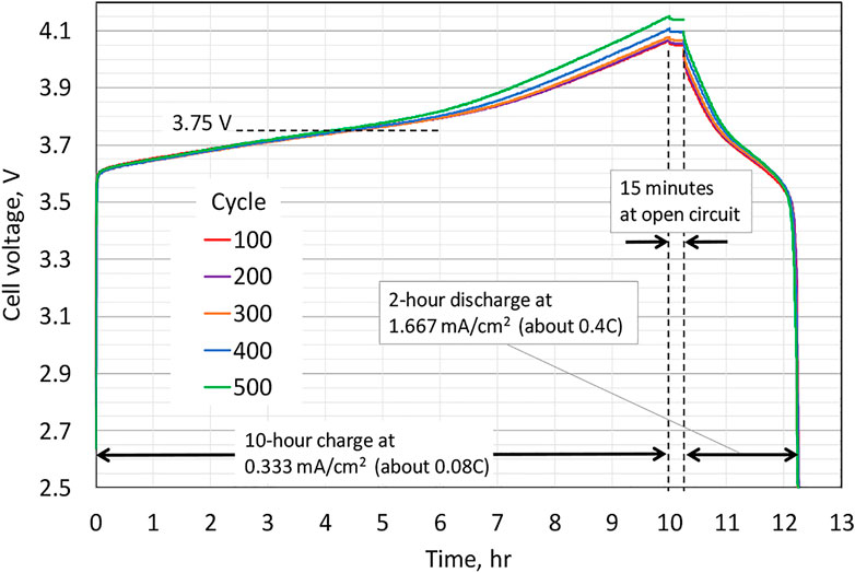
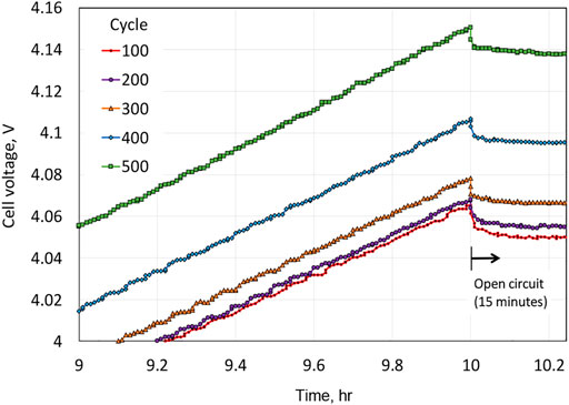
The experimental results are provided in Figure 2, along with a description of the protocol within the figure, which corresponds to, for each cycle, cell charging at a current density per electrode foil of 0.333 mA/cm² for 10 h (3.33 mAh/cm²), followed by a 15-min hold at the open circuit, and then subsequent discharge at 1.667 mA/cm² for 2 h (3.33 mAh/cm²).

FIGURE 2

FIGURE 2. Cell voltage vs. time for various cycles. The current density schedule is the same for each cycle. A horizontal line is shown for $V_{cell}=$ 3.75 V, corresponding to the $dq/d{V}_{cell}$ peaks shown in Figure 3.

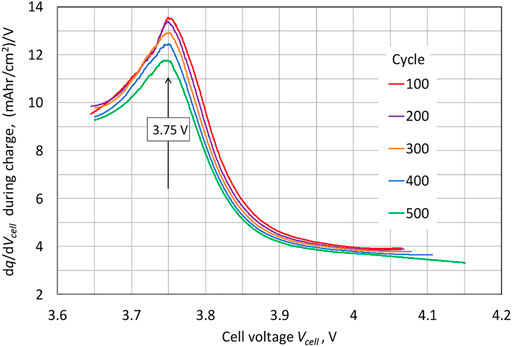
An important observation is that the potential continues to increase near the end of the charge for the Li||NMC622 cell. The differential voltage plot shown in Figure 3 indicates an approximate standard electrode potential for the NMC622 electrode of 3.75 V, the potential for the peak in the plot of $dq/d{V}_{cell}$ vs. $V_{cell}$ , which can be viewed as an approximate half-wave potential for the NMC622 electrode. Upon cycling, the peak magnitude diminishes continuously. A blow-up of the potential increase near the end of the charge and including the 15 min of open circuit stand after the charge is depicted in Figure 4. The sharp drop in potential upon transitioning from charge to open circuit is consistent with Ohmic-like resistance. The monotonic increase in the magnitude of the potential plateau at open circuit from cycle to cycle is consistent with the capacity loss of the NMC622 electrode, and this motivates our incorporating capacity degradation in our modeling of the NMC622 electrode (cation mixing). Lastly, we note that while the data plotted in Figure 2 through Figure 5 show a consistent trend, corresponding to increases in the cell potential during charge upon cycling, for cycles before cycle 100, the cell potential vs. time traces were similar to that of cycle 100 but did not show a consistent trend reflective of cell aging; hence, it took about 100 cycles to form the cell (i.e., for the cell to show a consistent aging trend during cycling). For this reason, in the Modeling section to follow, time $t = 0$ corresponds to the beginning of cycle 100.

FIGURE 3

FIGURE 3. The $dq/d{V}_{cell}$ vs. $V_{cell}$ curves were generated from the data shown in Figure 2.

FIGURE 4

FIGURE 4. The abscissa of Figure 2 is expanded about the transition from lithiation to open circuit.

FIGURE 5

FIGURE 5. Estimated open-circuit potential U for various cycles N. Symbols represent the potential after 15-min of open circuit for the data of Figure 2.

Mathematical Model

In this section, we present the equations used to model the cell shown schematically in Figure 6; i.e., a Li metal electrode at $z=0$ and a porous NMC622 electrode for $L_2\le z\le L_2+L$ .

FIGURE 6

FIGURE 6. Cell schematic. See the Nomenclature Index for the meaning of the variables shown.

Thermodynamics

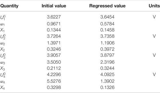
The thermodynamics for the lithium counter electrode at $z=0$ is simply $U_{Li}=0$ . We model the thermodynamics of the intercalation electrode with the multi-site, multi-reaction (MSMR) model (Verbrugge et al., 2017; Baker and Verbrugge, 2018; Baker et al., 2019; Baker and Verbrugge, 2021). The mole fraction of sites occupied by lithium in an NMC622 gallery j is x _j . Each species j is involved in an insertion reaction at the interface between the host particles and the electrolyte of the form

${\text{Li}}_{\text{liquid}}^{+}{+\text{ e}}_{\text{solid}}^{-}{+\text{ H}}_{j\text{,solid}}\rightleftarrows {\left(\text{Li}-\text{H}\right)}_{j\text{, solid}}.(1)$

Thus, for each species $j$ , a vacant host site ${\text{H}}_j$ can accommodate one Li leading to a filled host site ${\left(\text{Li}-\text{H}\right)}_j$ . The OCV (open-circuit voltage) for this reaction relative to a Li reference electrode is written as

$U_j=U_j^0+\frac{{\omega }_j}{f}\ln \left(\frac{X_j-x_j}{x_j}\right)\text{, }{x}_j=\frac{X_j}{1+\exp \left[f\left(U-U_j^0\right)/{\omega }_j\right]}\text{, and }x={\displaystyle \sum _j{x}_j},(2)$

where $f=\frac{F}{RT}$ , $X_j$ represents the total fraction of available host sites that can be occupied by species $j$ , ${\displaystyle \sum _j{X}_j}=1$ , $U_j^0$ can be viewed as a standard electrode potential for reaction j, and ${\omega }_j$ is a measure of the material’s disorder (Verbrugge et al., 2017) (larger ${\omega }_j$ yields broader peaks for reaction j in differential voltage spectroscopy plots). Local equilibrium is assumed, and

$U_1=U_2=U_j=U\left(x\right),(3)$

where the common potential $U\left(x\right)$ is the OCV of the NMC622 electrode with respect to a lithium reference.

Electrochemical Kinetics

Using the MSMR model (Verbrugge et al., 2017; Baker and Verbrugge, 2018; Baker et al., 2019), we express the kinetics of the insertion reaction are given as ¹

$\begin{array}{l}{i}_{s,j}=i_{0,j}[e^{\left(1-{\beta }_j\right)f{\eta }_s}-e^{-{\beta }_{j}f{\eta }_s}]\text{,}j={\displaystyle \sum i_{s,j}}\text{,}\\ {\eta }_s={\text{Φ}}_1-{\text{Φ}}_2-U\left(x\right)-j{R}_f\text{and }{i}_{0,j}=i_{0,j}^{ref}{\left(x_j\right)}^{{\omega }_j{\beta }_j}{(X_j-x_j)}^{{\omega }_j(1-{\beta }_j)},\end{array}(4)$

where ${\beta }_j$ are the symmetry factors for each reaction, ${\Phi }_1$ is the potential in the solid phase, and ${\Phi }_2$ is the potential in the electrolyte phase with respect to a lithium reference electrode. $R_f$ is a film resistance due to a surface layer on the electrode and $c_2$ is the salt concentration in the electrolyte. For the lithium counter electrode at $z=0$ (cf. Figure 6), the current density corresponds to the specified cell current density $i\left(t\right)$ :

$\begin{array}{l}i\left(t\right)=i_{0,Li}[e^{\left(1-{\beta }_{Li}\right)f{\eta }_{s,Li}}-e^{-{\beta }_{Li}f{\eta }_{s,Li}}]\text{,}\\ {\eta }_{s,Li}=-{\text{Φ}}_2-i\left(t\right)R_{f,Li}\left(t\right)\text{and }{i}_{0,Li}=i_{0,Li}^{ref}.\end{array}(5)$

We have referenced the potential at the current collector at $z=0$ ( ${{\Phi }_1|}_{z=0}=0$ ) which means that the cell potential will be ${\Phi }_1$ at the positive electrode’s current collector. In the microelectrode study of (Verbrugge and Koch, 1994), it was found that the Li/Li⁺ reaction is facile prior to Li degradation, after which the interfacial resistance was much larger and the current varied linearly with potential, consistent with an interfacial film resistance. Hence, we shall assume that the lithium charge–transfer reaction is facile, $i_{0,Li}^{ref}=\infty$ , and

${\eta }_{s,Li}=-{\text{Φ}}_2-i\left(t\right)R_{f,Li}\left(t\right)=0.(6)$

To approximate $R_{f,Li}\left(t\right)$ , we consider the irreversible degradation reaction

${2\text{Li}}_{solid}+\text{ Solvent }\stackrel{k}{\to }{\text{Li}}_2-\text{Solvent}\downarrow (7)$

and we express the rate of Li consumption as

$r_f=k{a}_{Li}^2{a}_{\text{Solvent}}.(8)$

We treat $a_{Li}\text{ and }{a}_{\text{Solvent}}$ as constants, as the metallic (bulk) Li electrodes remain at unit activity and we expect little variation in the solvent concentration. We shall treat $r_f$ as a constant, but it is likely that variations in this quantity arise due to changes with time, including changes in the film porosity, tortuosity, and interfacial contact area with the Li metal electrode. The resistance rise is modest in this work over several hundred cycles, so we deem this approximation to be appropriate. Hence, we assume the film thickness growth with time is linear, and that the film concentration $c_f$ and film resistivity ${\rho }_f$ are constants:

$\begin{array}{l}{c}_f\frac{d{L}_f}{dt}=r_f,L_f\left(t\right)=L_f\left(0\right)+\frac{r_f}{c_f}t,\text{and }\\ R_{f,Li}\left(t\right)=L_f\left(t\right){\rho }_f={\rho }_f\left[L_f\left(0\right)+\frac{r_f}{c_f}t\right].\end{array}(9)$

Also, the overall film sheet resistance $R_{f,Li}\left(t\right)$ that appears in the surface overpotential expression, Eq. 6, grows linearly with time.

Cation Mixing

As presented in the Introduction section, it is well known that the (irreversible) degradation of NMCs is caused in large part by transition metals (TMs) exchanging place with Li, often referred to as cation-mixing. For Ni in the TM layer exchanging with Li in the Li layer, the following formula is consistent with the x-ray diffraction results: ${{(\text{Li}}_{1-\text{δ}}{\text{Ni}}_{\text{δ}})}_{3\text{b}}{{(\text{Li}}_{\text{δ}}{\text{Ni}}_{\text{x}-\text{δ}}{\text{Mn}}_{\text{y}}{\text{Co}}_{1-\text{x}-\text{y}})}_{3\text{a}}{\text{O}}_2$ where $x+y+z=1$ and x, y, and z range between 0 and 1. To quote Julien et al. (2016), “The cation mixing corresponds to an antisite defect noted Ni_Li, which means that Ni²⁺ occupies a Li⁺ site that is compensated by the opposite, i.e., Li’_Ni, corresponding to a Li⁺ ion on a Ni²⁺ site preferentially close to it, to result in a neutral Ni_Li + Li’_Ni pair, with one Ni²⁺ ion on a 3b site plus one Li⁺ on a 3a site.”

For $\delta =0$ , there is no cation-mixing, there are no TMs in 3b sites, and there is no Li in 3a sites. For $\delta =1$ , cation-mixing is complete, and the material is inactive insofar as all Li sites are occupied by TMs.

We express the irreversible cation-mixing reaction as

${\text{M}}_{TM}{+\text{ Li}}_{Li}\stackrel{k_f}{\to }{\text{Li}}_{TM}{+\text{ M}}_{Li}.(10)$

The subscript TM refers to a transition metal (3a) site, and the subscript Li refers to a Li (3b) site. M refers to a TM. As mentioned in the Introduction section, of the three TMs—Ni, Mn, and Co—Ni is most prone to exchange with Li, although Mn and Co can as well. The fact that NMC622 has much more Ni than Mn or Co lends support to the use of a single equation, Eq. 10, instead of, for example, three separate equations for cation exchange involving Ni, Mn, or Co; a more sophisticated model would consider the individual rate expressions, as in expressions for Ni, Mn, and Co.

For NMC622, stoichiometry is given by LiMO₂, where the transition metal M is taken to represent Ni_0.6Mn_0.2Co_0.2. We assume that the total number of transition metal atoms in a particle is equal to the total number of transition metal sites in the same particle. By stoichiometry, $c_{TM}=c_T$ . The theoretical capacity of NMC622 is 276 mAh/(g Ni_0.6Mn_0.2Co_0.2), but the actual capacity is typically about 180 mAh/g (NohNoh et al., 2013). Hence, the moles of active Li sites to the total Li sites is typically about ${\epsilon }_{1F}\approx 180/276=0.65$ . For cation exchange, we consider only those Li sites that are active, and, consequently, only those TMs near an active Li site. To be explicit, the following concentrations are of interest:

$\begin{array}{l}\underset{{\epsilon }_{1,F}}{\underbrace{\left(\frac{\text{mol active Li sites}}{\text{mol total Li sites}}\right)}}\underset{c_T}{\underbrace{\left(\frac{\text{mol total Li sites}}{{\text{cm}}^3}\right)}}\underset{x}{\underbrace{\left(\frac{\text{mol Li in active Li sites}}{\text{mol active Li sites}}\right)}}=\frac{\text{mol Li in active Li sites}}{{\text{cm}}^3},\\ \underset{{\epsilon }_{1,F}}{\underbrace{\left(\frac{\text{mol active Li sites}}{\text{mol total Li sites}}\right)}}\underset{c_T}{\underbrace{\left(\frac{\text{mol total Li sites}}{{\text{cm}}^3}\right)}}\underset{x_{TM}}{\underbrace{\left(\frac{\text{mol TM in active Li sites}}{\text{mol active Li sites}}\right)}}=\frac{\text{mol TM in active Li sites}}{{\text{cm}}^3},\\ \underset{{\epsilon }_{1,F}}{\underbrace{\left(\frac{\text{mol active TM sites}}{\text{mol total TM sites}}\right)}}\underset{c_{TM}=c_T}{\underbrace{\left(\frac{\text{mol total TM sites}}{{\text{cm}}^3}\right)}}\underset{X_{TM}}{\underbrace{\left(\frac{\text{mol TM in active TM sites}}{\text{mol active TM sites}}\right)}}=\frac{\text{mol TM in active TM sites}}{{\text{cm}}^3}.\end{array}$

Conservation of transition metals yields

${\epsilon }_{1F}{c}_{TM}(1-X_{TM})={\epsilon }_{1F}{c}_T{x}_{TM}\text{ and }{X}_{TM}=1-x_{TM},(11)$

and we construct our rate expression for the cation-mixing reaction (10) as

$r_{CM}=k_f\left({\epsilon }_{1F}{c}_T{X}_{TM}\right)\left({\epsilon }_{1F}{c}_{T}x\right)=k_f{\left({\epsilon }_{1F}{c}_T\right)}^2{X}_{TM}x=k_f{\left({\epsilon }_{1F}{c}_T\right)}^2(1-x_{TM})x,(12)$

where $r_{CM}$ has units of, for example, mol/cm³-s.

Material Balance in the Porous-Electrode Particles

The cation species is assumed to be immobile and cannot diffuse within the host material. Volumetric expansion is neglected, so that $c_T$ is assumed to be constant, and we treat primary particles, i.e., we do not consider any porosity or tortuosity within a particle. A material balance on all sites yields

$\begin{array}{l}x+x_H+x_{TM}=1,\\ c_T\frac{\partial x}{\partial \tau }=-\nabla \cdot N-r_{CM},\\ c_T\frac{\partial x_H}{\partial \tau }=-\nabla \cdot N_H,\\ c_T\frac{\partial x_{TM}}{\partial \tau }=r_{CM},\\ -\nabla \cdot \left(N+N_H\right)=0,\end{array}(13)$

where $N$ and $N_H$ are the fluxes of lithium occupied and vacant sites, respectively.

By symmetry, $N+N_H=0$ at the particle center and it follows that $N+N_H=0$ everywhere.

The Gibbs–Duhem relation (Guggenheim, 1977; Lasdon et al., 1978; Fylstra et al., 1998; Bizeray et al., 2016) states that at constant temperature and pressure the chemical potentials of the individual species satisfy

$x\nabla \mu +\left(1-x_{TM}-x\right)\nabla {\mu }_H+x_{TM}\nabla {\mu }_{TM}=0.(14)$

We shall assume that other than blocking Li sites in the Li layer, the transition metals do not interact with Li in the Li layer and that $\nabla {\mu }_{TM}=0$ . This assumption can be invalid if the transition metal concentrations get large in the Li layer and the mixing reaction is facile, unlike the data we treat in this work. Eq. 14 becomes

$\begin{array}{l}x\nabla \mu +\left(1-x_{TM}-x\right)\nabla {\mu }_H=0,\\ \nabla {\mu }_H=-\frac{x}{\left(1-x_{TM}-x\right)}\nabla \mu .\end{array}(15)$

Substitutional diffusion in a lithium host material consisting of two species, the Li-occupied and unoccupied sites, then satisfies (Baker and Verbrugge, 2012)

$F\nabla U=\nabla \mu -\nabla {\mu }_H=\frac{1-x_{TM}}{1-x_{TM}-x}\nabla \mu (16)$

and

$\begin{array}{l}N=-c_{T}x\frac{D}{RT}\nabla \mu +x\left(N+N_H\right)=-c_{T}x\frac{D}{RT}\nabla \mu ,\\ N=-c_{T}x\frac{F}{RT}D\frac{\left(1-x-x_{TM}\right)}{\left(1-x_{TM}\right)}\nabla U,\end{array}(17)$

where $D$ is a diffusion coefficient, which we will assume to be constant, and $c_T$ is the total concentration of sites occupied by either lithium, transition metals, or vacant sites. We note that in principle, the chemical potential $\mu$ has a dependence on $x_{TM}$ , but this dependence can be subsumed in the reference state as long as $x_{TM}$ is constant. (See also the aforementioned assumption concerning the Gibbs–Duhem equation).

At this point, it is convenient to introduce the mole fraction

$\tilde{x}=\frac{x}{\left(1-x_{TM}\right)}(18)$

of sites in the Li layer unoccupied by the transition metal but occupied by Li. Eq. 17 then becomes

$\text{N}=-c_T\left(1-x_{TM}\right)\frac{F}{RT}D\tilde{x}\left(1-\tilde{x}\right)\nabla U.(19)$

The material balance of lithium in the solid phase, including loss of Li due to cation mixing, is given by

$\begin{array}{c}\frac{\partial }{\partial t}\left(\left(1-x_{TM}\right)\tilde{x}\right)=-\nabla \cdot \text{N}-r_{CM}=-\nabla \cdot \left[\left(1-x_{TM}\right)\tilde{x}\left(1-\tilde{x}\right)fD\nabla U\right]-r_{CM},\\ =-\frac{1}{r^2}\frac{\partial }{\partial r}\left[r^2\left(1-x_{TM}\right)x\left(1-x\right)fD\frac{\partial U}{\partial r}\right]-k_f{\epsilon }_{1F}^2{c}_T{(1-x_{TM})}^2\tilde{x},\end{array}(20)$

where we have assumed that the NMC particles are spherical. In this work, we do not consider the potential for changes in material properties that may result from cation mixing.

Boundary conditions for Eq. 20 are

$\begin{array}{l}\frac{\partial \tilde{x}}{\partial r}=0\text{ at }r=0,\\ c_T\left(1-x_{TM}\right)\tilde{x}\left(1-\tilde{x}\right)fD\frac{\partial U}{\partial r}=\frac{j}{F}\text{ at }r=a,\end{array}(21)$

where a is the particle radius and $j$ is defined in Eq. 4.

We also require a material balance for the immobile transition metal ions in the lithium layer of the particles:

$c_T\frac{\partial x_{TM}}{\partial t}=r_{CM}=k_f{\left({\epsilon }_{1F}{c}_T\right)}^2(1-x_{TM})x=k_f{\left({\epsilon }_{1F}{c}_T\right)}^2{(1-x_{TM})}^2\tilde{x}.(22)$

We close this subsection by noting that the maximum equilibrium (areal) capacity Q of the electrode diminishes due to cation mixing:

$Q\left(t\right)=Q_0\left(1-x_{TM}\left(t\right)\right),Q_0=FL{\epsilon }_1{\epsilon }_{1F}{c}_T.(23)$

Porous Electrode and Separator Equations

The following equations apply (Baker and Verbrugge, 2021):

$i_1=-\frac{{\epsilon }_1{\kappa }_1}{{\text{Γ}}_1}\frac{\partial {\text{Φ}}_1}{\partial z},(24)$

$\frac{\partial i_1}{\partial z}=-{\epsilon }_{1,F}{a}_{s}j,(25)$

$\begin{array}{l}{i}_2=\frac{{\epsilon }_{2,E}{\kappa }_2\left(c_2\right)}{{\text{Γ}}_{2,E}}\left[-\frac{\partial {\text{Φ}}_2}{\partial z}+\frac{2RT}{F}\left(1+\frac{d\ln f_{\pm }}{d\ln c_2}\right)\left(1-t_{+}^0\right)\frac{\partial }{\partial z}\ln \left(c_2\right)\right]\left(\text{electrode}\right)\text{,}\\ i_2=\frac{{\epsilon }_{2,S}{\kappa }_2\left(c_2\right)}{{\text{Γ}}_{2,S}}\left[-\frac{\partial {\text{Φ}}_2}{\partial z}+\frac{2RT}{F}\left(1+\frac{d\ln f_{\pm }}{d\ln c_2}\right)\left(1-t_{+}^0\right)\frac{\partial }{\partial z}\ln \left(c_2\right)\right]\left(\text{separator}\right)\text{,}\end{array}(26)$

$\begin{array}{l}\frac{\partial i_2}{\partial z}={\epsilon }_{1,F}{a}_{s}j\left(\text{electrode}\right)\text{,}\\ i_2=i\left(t\right)\left(\text{separator}\right)\text{,}\end{array}(27)$

$\begin{array}{l}\frac{\partial c_2}{\partial t}=\frac{\partial }{\partial z}\left[\frac{D_2\left(c_2\right)}{{\text{Γ}}_{2,E}}\frac{\partial c_2}{\partial z}+\left(1-t_{+}^0\right)\frac{i_2}{{\epsilon }_{2,E}F}\right]\left(\text{electrode}\right)\text{,}\\ \frac{\partial c_2}{\partial t}=\frac{\partial }{\partial z}\left[\frac{D_2\left(c_2\right)}{{\text{Γ}}_{2,S}}\frac{\partial c_2}{\partial z}+\left(1-t_{+}^0\right)\frac{i_2}{{\epsilon }_{2,S}F}\right]\left(\text{separator}\right)\text{.}\end{array}(28)$

The superficial current density in the solid phase of the porous electrode is given as $i_1$ and in the electrolyte phase as $i_2$ . Note that the porosity and tortuosity can (and usually do) differ in the separator and the electrode. The meaning of the remaining parameters can be found in the Nomenclature listing.

At $z=0$ , the flux of the anion $N_2$ vanishes,

$N_2=-\frac{{\epsilon }_2{D}_2\left(c_2\right)}{{\text{Γ}}_2}\frac{\partial c_2}{\partial z}-\left(1-t_{+}^0\right)\frac{i_2}{F}=0,(29)$

and Eq. 6 can also be used to determine ${\Phi }_2\left(z=0\right)$ .

At $z=L_2$ , the separator interface with the porous electrode,

$i_1=0.(30)$

In addition, the variables ${\Phi }_2,\text{ and }{c}_2$ , the liquid phase current $i_2$ , and the salt flux $N_2$ are continuous at this interface.

At $z=L_2+L$ , the current collector, the current density $i\left(t\right)$ is specified, and

$\begin{array}{l}{N}_2=i_2=0,\\ i_1=i\left(t\right).\end{array}(31)$

Because we are interested in solutions at low current densities, we write the current density as

$i\left(t\right)=\frac{I\left(\frac{t}{t_0}\right)}{t_0},(32)$

where $t_0$ is the time taken for a single cycle. In this way, we can use the perturbation analysis to determine approximate solutions for current density in the limit as $t_0\to \infty$ and $i\left(t\right)$ is small. Note that $I$ has the units of capacity $Q$ per unit geometric area.

Non-dimensionalization and Scaling

Please refer to the Notation listing for definitions. To put these equations in a dimensionless form, we introduce the following resistances:

$\begin{array}{l}{R}_e=\frac{{\text{Γ}}_{2,E}L}{{\epsilon }_{2,E}{\kappa }_2\left(c_0\right)},R_{sep}=\frac{{\text{Γ}}_{2,S}{L}_2}{{\epsilon }_{2,S}{\kappa }_2\left(c_0\right)},R_f=\frac{1}{f{i}_s}{\overline{R}}_f,\\ R_d=\frac{a}{fFL{a}_s{\epsilon }_{1,F}D{c}_T}=\frac{a^2}{3fFL{\epsilon }_1{\epsilon }_{1,F}D{c}_T},R_s=\frac{{\text{Γ}}_{1}L}{{\epsilon }_1{\kappa }_1},\\ R_{e,diff}=\frac{{\text{Γ}}_{2,E}L}{{\epsilon }_{2,E}fF{D}_2\left(c_0\right)c_0},R_k=\frac{1}{fL{a}_s{\epsilon }_{1,F}{i}_s}=\frac{a}{3fL{\epsilon }_1{\epsilon }_{1,F}{i}_s},\\ R_{k,Li}=\frac{1}{f{i}_{0,Li}^{ref}},{\widehat{R}}_{Li,f,init}={\rho }_f{L}_f\left(0\right),{\widehat{R}}_{Li,f}={\rho }_f\frac{r_f}{c_f}{t}_0.\end{array}(33)$

We will use the following dimensionless quantities:

$\begin{array}{l}z=\{\begin{array}{c}{L}_2\overline{z}\\ L\left(\overline{z}-1\right)+L_2\end{array}\begin{array}{c}\text{for}\overline{z}\le 1\text{in}\text{the}\text{separator}\\ \text{for}1\le \overline{z}\le 2\text{in}\text{the}\text{electrode}\end{array},\\ c_2=c_0{\overline{c}}_2,{\overline{D}}_2=\frac{D_2\left(c_2\right)}{D_2\left(c_0\right)},\alpha =\frac{t_0}{t_1},t_1=\frac{1}{k_f{\epsilon }_{1F}^2{c}_T},{\overline{\kappa }}_2=\frac{{\kappa }_2\left(c_2\right)}{{\kappa }_2\left(c_0\right)},\\ r=a\overline{r},\tau =\frac{t}{t_0},\gamma =\frac{a^2}{D{t}_0},\tilde{\gamma }=\frac{{\text{Γ}}_{2,E}{L}^2}{D_2\left(c_0\right)t_0},N_2=\frac{1}{f{R}_{e,diff}}{\overline{N}}_2,\\ i_2=\frac{1}{f{R}_e}{\overline{i}}_2,i_1=\frac{1}{f{R}_s}{\overline{i}}_1,i=\frac{1}{f{R}_s}\overline{i},{\text{Φ}}_k=\frac{{\overline{\text{Φ}}}_k}{f},U=\frac{\overline{U}}{f},\\ i_{s,k}=i_s{\overline{i}}_{s,k},i_{0,k}=i_s{\overline{i}}_{0,k},j=i_s\overline{j},i_{0,Li}=i_s{\overline{i}}_{0,Li},\overline{I}=\frac{I}{Q_0},\\ \widehat{\kappa }=\frac{1}{1+2\frac{R_{e,diff}}{R_e}{\left(1+\frac{d\ln f_{\pm }}{d\ln c_2}\right)|}_{c_2=c_0}{\left(1-t_{+}^0\right)}^2}.\end{array}(34)$

The scaling parameter $i_s$ should be chosen to appropriately scale the interfacial current $j$ . We use $i_s=i_{\mathrm{0,1}}^{ref}$ . We will be interested in two different time scales. To calculate the fluctuations in mole fraction $x$ over the course of a single cycle, we are primarily interested in diffusion, and the material balance Eq. 22 for the cation only varies on a much larger time scale. It follows that, in the course of a single cycle, $x_{TM}$ can be regarded as constant. This is realized mathematically by assuming that $\alpha <<1$ , where $\alpha =t_0/t_1$ is the ratio of single cycle time to the cation reaction time scale. Thus, over the course of a single cycle, we are justified in dropping terms of order $\alpha$ and the mole fraction $\tilde{x}$ becomes the preferred variable, because $x_{TM}$ is constant to order $\alpha$ . In contrast, the material balance (22) for the cation changes on time scales $\tau =O\left(1/\alpha \right)$ , where O refers to order, and it is no longer acceptable to drop terms of order $\alpha$ . On this time scale, the variable $x$ is the preferred choice, and $x_{TM}$ can no longer be viewed as a constant.

The resulting dimensionless equations in the electrode and separator are

${\overline{i}}_1=\frac{\partial {\overline{\text{Φ}}}_1}{\partial \overline{z}},(35)$

$\frac{\partial {\overline{i}}_1}{\partial \overline{z}}=-\frac{R_s}{R_k}\overline{j},(36)$

$\begin{array}{l}{\overline{i}}_2={\overline{\kappa }}_2\left[-\frac{\partial {\overline{\text{Φ}}}_2}{\partial \overline{z}}+\left(1+\frac{d\ln f_{\pm }}{d\ln c_2}\right)\left(1-t_{+}^0\right)\frac{\partial }{\partial \overline{z}}\ln \left({\overline{c}}_2\right)\right]\left(\text{electrode}\right)\text{,}\\ {\overline{i}}_2=\frac{R_e}{R_{sep}}{\overline{\kappa }}_2\left[-\frac{\partial {\overline{\text{Φ}}}_2}{\partial \overline{z}}+\left(1+\frac{d\ln f_{\pm }}{d\ln c_2}\right)\left(1-t_{+}^0\right)\frac{\partial }{\partial \overline{z}}\ln \left({\overline{c}}_2\right)\right]\left(\text{separator}\right)\text{,}\end{array}(37)$

$\begin{array}{l}\frac{\partial {\overline{i}}_2}{\partial \overline{z}}=\frac{R_e}{R_k}\overline{j}\left(\text{electrode}\right)\text{,}\\ {\overline{i}}_2=\frac{R_{sep}}{R_s}\overline{i}\left(\text{separator}\right)\text{,}\end{array}(38)$

$\begin{array}{l}\tilde{\gamma }\frac{\partial {\overline{c}}_2}{\partial \tau }=\frac{\partial }{\partial \overline{z}}\left[{\overline{D}}_2\frac{\partial {\overline{c}}_2}{\partial \overline{z}}+\frac{\left(1-t_{+}^0\right)R_{e,diff}}{R_e}{\overline{i}}_2\right]\left(\text{electrode}\right)\text{,}\\ \frac{{\epsilon }_{2S}}{{\epsilon }_{2E}}\frac{L_2}{L}\tilde{\gamma }\frac{\partial {\overline{c}}_2}{\partial \tau }=\frac{R_e}{R_{sep}}\frac{\partial }{\partial \overline{z}}\left({\overline{D}}_2\frac{\partial {\overline{c}}_2}{\partial \overline{z}}\right)\left(\text{separator}\right)\text{.}\end{array}(39)$

The dimensionless equations for the material balances within the solid particles are

$\begin{array}{l}\frac{\partial \tilde{x}}{\partial \tau }=-\frac{1}{\gamma }\frac{1}{{\overline{r}}^2}\frac{\partial }{\partial \overline{r}}\left[{\overline{r}}^2\tilde{x}\left(1-\tilde{x}\right)\frac{d\overline{U}}{d\tilde{x}}\frac{\partial \tilde{x}}{\partial \overline{r}}\right]+O\left(\alpha \right),\\ \frac{\partial x_{TM}}{\partial \tau }=0+O\left(\alpha \right),\end{array}(40)$

where we will drop terms of order $\alpha$ . Boundary conditions are given as

$\begin{array}{ll}\tilde{x}=\tilde{x}\left(N\right)\text{ and }{x}_{TM}=x_{TM}\left(N\right)\hfill & \tau =N\hfill \\ \left(1-x_{TM}\right)\tilde{x}\left(1-\tilde{x}\right)\frac{d\overline{U}}{d\tilde{x}}\frac{\partial x}{\partial \overline{r}}=\frac{R_d}{R_k}\overline{j}\hfill & \overline{r}=1\hfill \\ \frac{\partial x}{\partial \overline{r}}=0\hfill & \overline{r}=0\hfill \end{array},(41)$

where $\tau =N$ , an integer, denotes the start of a cycle. In the aforementioned equations, it is assumed that the OCV $\overline{U}$ is a function of $\tilde{x}$ , which does not change, even as $x_{TM}$ changes.

The dimensionless equations for the electrochemical reactions within the porous electrode are

$\begin{array}{l}{\overline{i}}_{s,j}={\overline{i}}_{0,j}[e^{\left(1-{\beta }_j\right){\overline{\eta }}_s}-e^{-{\beta }_j{\overline{\eta }}_s}]\text{,}\overline{j}={\displaystyle \sum _{j=1}^J{\overline{i}}_{s,j}},\\ {\overline{i}}_{0,j}={\overline{i}}_{0,j}^{ref}{\left(x_j\right)}^{{\omega }_j{\beta }_j}{(X_j-x_j)}^{{\omega }_j(1-{\beta }_j)}\text{ and }{\overline{\eta }}_s={\overline{\text{Φ}}}_1-{\overline{\text{Φ}}}_2-\overline{U}-\overline{j}{\overline{R}}_f.\end{array}(42)$

Also, at the Li electrode are

$\begin{array}{l}\overline{i}=\frac{R_s}{R_{k,Li}}{\overline{i}}_{0,Li}[e^{\left(1-{\beta }_{Li}\right){\overline{\eta }}_{s,Li}}-e^{-{\beta }_{Li}{\overline{\eta }}_{s,Li}}]\text{,}\\ {\overline{i}}_{0,Li}={\overline{i}}_{0,Li}^{ref}\text{ and }{\overline{\eta }}_{s,Li}=-{\overline{\text{Φ}}}_2-\overline{i}\left(\frac{{\widehat{R}}_{Li,f,init}}{R_s}+\frac{{\widehat{R}}_{Li,f}}{R_s}\tau \right).\end{array}(43)$

The following relationship is used in deriving Eq. 45 and will be used elsewhere as well.

$\frac{Q_0}{t_0}=\frac{\gamma }{3f{R}_d}.(44)$

At the current collector, the current is specified, and using Eq. 32, we can write

$\begin{array}{l}\overline{i}={\overline{i}}_1\left(\overline{z}=2\right)=\frac{\gamma }{3}\frac{R_s}{R_d}\overline{I}\left(\tau \right),\\ \overline{i}={\overline{i}}_1+\frac{R_s}{R_e}{\overline{i}}_2.\end{array}(45)$

The cell voltage becomes

${\overline{V}}_{cell}={\overline{\text{Φ}}}_1\left(\overline{z}=2\right)-\frac{R_c}{R_s}{\overline{i}}_1\left(\overline{z}=2\right).(46)$

In addition,

${\overline{i}}_2\left(\overline{z}=2\right)={\overline{N}}_2\left(\overline{z}=2\right)=0,(47)$

where

${\overline{N}}_2=\{\begin{array}{c}-\left[{\overline{D}}_2\frac{\partial {\overline{c}}_2}{\partial \overline{z}}+\frac{R_{e,diff}}{R_e}\left(1-t_{+}^0\right){\overline{i}}_2\right]\text{ in the electrode}\\ -\left[\frac{R_e}{R_{sep}}{\overline{D}}_2\frac{\partial {\overline{c}}_2}{\partial \overline{z}}+\frac{R_{e,diff}}{R_{sep}}\left(1-t_{+}^0\right){\overline{i}}_2\right]\text{ in the separator}\end{array}.(48)$

At the interface between the separator and the working electrode,

${\overline{i}}_1\left(\overline{z}=1\right)=0,(49)$

and the variables ${\overline{\Phi }}_2,\text{ and }{\overline{c}}_2$ , the liquid phase current ${\overline{i}}_2$ , and the salt flux ${\overline{N}}_2$ are continuous at this interface.

In addition,

${\overline{N}}_2\left(\overline{z}=0\right)=0.(50)$

Integration Formulas That Simplify the Modeling of Cation Mixing

This section is concerned with the changes in $x_{TM}$ over time spans of many cycles, so that $\tau =O\left(1/\alpha \right)$ . As such, the mole fraction $x$ , instead of $\tilde{x}$ , is used, and the terms of order $\alpha$ can no longer be ignored. However, terms of order ${\alpha }^2$ will be ignored. With these changes, Eq. 40 can be rewritten as

$\begin{array}{l}\frac{\partial x}{\partial \tau }=-\frac{1}{\gamma }\frac{1}{{\overline{r}}^2}\frac{\partial }{\partial \overline{r}}\left[{\overline{r}}^{2}x\left(1-x\right)\frac{d\overline{U}}{dx}\frac{\partial x}{\partial \overline{r}}\right]-\alpha x\left(1-x_{TM}\right),\\ \frac{\partial x_{TM}}{\partial \tau }=\alpha x\left(1-x_{TM}\right).\end{array}(51)$

If one integrates the first of Eq. 51 over the spherical particle, one obtains:

$\gamma {\displaystyle \underset{0}{\overset{1}{\int }}\left(\frac{\partial x}{\partial \tau }+\alpha \left(1-x_{TM}\right)x\right){\overline{r}}^{2}d\overline{r}}=-{\overline{N}}_1\left(\overline{r}=1\right)={-x\left(1-x\right)\frac{d\overline{U}}{dx}\frac{\partial x}{\partial \overline{r}}|}_{\overline{r}=1}=-\frac{R_d}{R_k}\overline{j}.(52)$

If one then integrates Eq. 52 over the porous electrode and uses Eqs 36, 45, one obtains

$\gamma {\displaystyle \underset{1}{\overset{2}{\int }}{\displaystyle \underset{0}{\overset{1}{\int }}\left(\frac{\partial x}{\partial \tau }+\alpha \left(1-x_{TM}\right)x\right){\overline{r}}^{2}d\overline{r}d\overline{z}}}=-\frac{R_d}{R_k}{\displaystyle \underset{1}{\overset{2}{\int }}\overline{j}}d\overline{z}=\frac{R_d}{R_s}{\overline{i}}_1(\overline{z}=2)=\frac{R_d}{R_s}\overline{i}=\frac{\gamma }{3}\overline{I}.(53)$

A time integrated form of Eq. 53 yields

$\begin{array}{l}{\displaystyle \underset{1}{\overset{2}{\int }}{\displaystyle \underset{0}{\overset{1}{\int }}x\left(\overline{r},\overline{z},\tau +1\right){\overline{r}}^{2}d\overline{r}d\overline{z}}}+\alpha {\displaystyle \underset{\tau }{\overset{\tau +1}{\int }}{\displaystyle \underset{1}{\overset{2}{\int }}{\displaystyle \underset{0}{\overset{1}{\int }}\left(1-x_{TM}\right)x{\overline{r}}^{2}d\overline{r}}d\overline{z}}d\tau }\\ =\frac{1}{3}{\displaystyle \underset{\tau }{\overset{\tau +s}{\int }}\overline{I}\left(\tau \right)d\tau }+{\displaystyle \underset{1}{\overset{2}{\int }}{\displaystyle \underset{0}{\overset{1}{\int }}x\left(\overline{r},\overline{z},\tau \right){\overline{r}}^{2}d\overline{r}d\overline{z}.}}\end{array}(54)$

For any function $f\left(\overline{r},\overline{z},\tau \right)$ , we will write

$\overline{f}\left(\tau \right)={\displaystyle \underset{\tau }{\overset{\tau +1}{\int }}{\displaystyle \underset{0}{\overset{1}{\int }}{\displaystyle \underset{0}{\overset{1}{\int }}f\left(\overline{r},\overline{z},s\right){\overline{r}}^{2}d\overline{r}}d\overline{z}}}ds.(55)$

This is the average value of $f$ in the entire cell over one cycle. We now integrate the various pieces of Eq. 53, starting with

$\overline{\frac{\partial x}{\partial \tau }}={\displaystyle \underset{\tau }{\overset{\tau +1}{\int }}{\displaystyle \underset{0}{\overset{1}{\int }}{\displaystyle \underset{0}{\overset{1}{\int }}\frac{\partial x}{\partial s}{\overline{r}}^{2}d\overline{r}d\overline{z}}}}ds={\displaystyle \underset{0}{\overset{1}{\int }}{\displaystyle \underset{0}{\overset{1}{\int }}x\left(\tau +1\right){\overline{r}}^{2}d\overline{r}d\overline{z}}}-{\displaystyle \underset{0}{\overset{1}{\int }}{\displaystyle \underset{0}{\overset{1}{\int }}x\left(\tau \right){\overline{r}}^{2}d\overline{r}d\overline{z}}}.(56)$

However,

$\frac{\partial \overline{x}}{\partial \tau }=\frac{\partial }{\partial \tau }{\displaystyle \underset{\tau }{\overset{\tau +1}{\int }}{\displaystyle \underset{0}{\overset{1}{\int }}{\displaystyle \underset{0}{\overset{1}{\int }}x{\overline{r}}^{2}d\overline{r}d\overline{z}}}}ds={\displaystyle \underset{0}{\overset{1}{\int }}{\displaystyle \underset{0}{\overset{1}{\int }}x\left(\tau +1\right){\overline{r}}^{2}d\overline{r}d\overline{z}}}-{\displaystyle \underset{0}{\overset{1}{\int }}{\displaystyle \underset{0}{\overset{1}{\int }}x\left(\tau \right){\overline{r}}^{2}d\overline{r}d\overline{z}}}=\overline{\frac{\partial x}{\partial \tau }}.(57)$

If one assumes that the total current passed in each cycle is zero,

${\displaystyle \underset{\tau }{\overset{\tau +1}{\int }}\overline{I}\left(\tau \right)d\tau }=0(58)$

then Eq. 54 becomes

${\displaystyle \underset{1}{\overset{2}{\int }}{\displaystyle \underset{0}{\overset{1}{\int }}x\left(\overline{r},\overline{z},\tau +1\right){\overline{r}}^{2}d\overline{r}d\overline{z}}}+\alpha {\displaystyle \underset{\tau }{\overset{\tau +1}{\int }}{\displaystyle \underset{1}{\overset{2}{\int }}{\displaystyle \underset{0}{\overset{1}{\int }}\left(1-x_{TM}\right)x{\overline{r}}^{2}d\overline{r}}d\overline{z}}d\tau }={\displaystyle \underset{1}{\overset{2}{\int }}{\displaystyle \underset{0}{\overset{1}{\int }}x\left(\overline{r},\overline{z},\tau \right){\overline{r}}^{2}d\overline{r}d\overline{z}}},(59)$

and using Eq. 57,

$\frac{\partial \overline{x}}{\partial \tau }=-\alpha \overline{\left(1-x_{TM}\right)x}.(60)$

Eqs 51, 60 now imply that, to the leading order in $\alpha$ , both $\overline{x}$ and $x_{TM}$ are constant over a single cycle so that

$\frac{\partial \overline{x}}{\partial \tau }=-\alpha \left(1-{\overline{x}}_{TM}\right)\overline{x}+O\left({\alpha }^2\right),(61)$

and similarly,

$\frac{\partial {\overline{x}}_{TM}}{\partial \tau }=\alpha \left(1-{\overline{x}}_{TM}\right)\overline{x}+O\left({\alpha }^2\right).(62)$

More precise statements that are valid over many cycles can be made by summing Eq. 51 and then averaging over the entire cell and over time:

$\begin{array}{l}\frac{\partial }{\partial \tau }\left(\overline{x}+{\overline{x}}_{TM}\right)=0,\\ \overline{x}\left(\tau \right)+{\overline{x}}_{TM}\left(\tau \right)=\overline{x}\left(0\right)+{\overline{x}}_{TM}\left(0\right),\end{array}(63)$

where $\overline{x}\left(0\right)\text{ and }{\overline{x}}_{TM}\left(0\right)$ are the initial values for $\overline{x}\text{ and }{\overline{x}}_{TM}$ . It now follows from Eq. 61 that

$\frac{d\overline{x}}{d\tau }=-\alpha \left(\chi +\overline{x}\right)\overline{x}+O\left({\alpha }^2\right),\chi =1-{\overline{x}}_{TM}\left(0\right)-\overline{x}\left(0\right),(64)$

which can be integrated to yield

$\overline{x}\left(\tau \right)=\frac{\overline{x}\left(0\right)\chi e^{-\alpha \chi \tau }}{1-{\overline{x}}_{TM}\left(0\right)-\overline{x}\left(0\right)e^{-\alpha \chi \tau }}+O\left({\alpha }^2\tau \right).(65)$

The approximation (65) is valid, even when $\tau >>1$ , which means that it can be used to approximate capacity loss over many cycles. In particular, the error in the approximation (65) is formally much smaller than the one in the limit of $\alpha <<1$ and for $\tau <<1/{\alpha }^2$ . Both assumptions are valid in this work. The initial condition $\overline{x}\left(0\right)$ in the aforementioned equation is the average SOC in the initial cycle.

Last, we can now express the areal Coulombic capacity. Substituting Eq. 65 into Eq. 23, we obtain

$\begin{array}{c}Q\left(\tau \right)=Q_0(1-{\overline{x}}_{TM})=FL{\epsilon }_1{\epsilon }_{1F}{c}_T\left(1-{\overline{x}}_{TM}\right),\\ =FL{\epsilon }_1{\epsilon }_{1F}{c}_T\chi \left(\frac{1-{\overline{x}}_{TM}\left(0\right)}{1-{\overline{x}}_{TM}\left(0\right)-\overline{x}\left(0\right)e^{-\alpha \chi \tau }}\right)+O\left({\alpha }^2\tau \right).\end{array}(66)$

Low-Current Perturbation Solution

In this section, we return to the problem of approximating cell voltage over the period of one cycle. Thus, we again return to the mole fraction $\tilde{x}$ , instead of $x$ , we consider $x_{TM}$ to be constant over a cycle, and we will drop terms of order $\alpha$ . Our main tool is the perturbation analysis developed in (Baker and Verbrugge, 2021). This starts with the assumption ² that $t_0$ is sufficiently large that both $\gamma ,\tilde{\gamma }<<1$ . In addition, we assume that $\alpha <<1$ and derive leading order expressions in the limit of small $\alpha$ as well. Our goal is to derive a perturbation approximation for the cell voltage during the course of a single cycle, and the dimensionless time $\tau =t/t_0$ changes by only one in the course of a cycle. Thus, for treating a cycle, we can drop the order $\alpha$ term in Eq. 40, obtaining

$\frac{\partial \tilde{x}}{\partial \tau }=-\frac{1}{\gamma }\frac{1}{{\overline{r}}^2}\frac{\partial }{\partial \overline{r}}\left[{\overline{r}}^2\tilde{x}\left(1-\tilde{x}\right)\frac{d\overline{U}}{d\tilde{x}}\frac{\partial \tilde{x}}{\partial \overline{r}}\right]+O\left(\alpha \right)\text{ and }\frac{\partial x_{TM}}{\partial \tau }=O\left(\alpha \right).(67)$

Also, we assume that $x_{TM}$ is constant to leading order in $\alpha$ . As was done in (Baker and Verbrugge, 2021), we can expand each dependent variable in, for example, the total mole fraction $x$ of filled Li sites in the NMC622 Li layer expressed as

$\tilde{x}={\tilde{x}}_0+\gamma {\tilde{x}}_1+{\gamma }^2{\tilde{x}}_2+\mathrm{...}(68)$

where … represents higher order terms in the expansion. The leading order term ${\tilde{x}}_0$ in Eq. 68 is the equilibrium state which arises when the current in Eq. 32 is tending to zero as $t_0$ tends to infinity, and it thus varies with time $\tau =t/t_0$ but has no position dependence, unlike the higher order terms.

We now present the perturbation solution derived using the procedures described in the work of Baker and Verbrugge (2021).

$\begin{array}{l}{\overline{V}}_{cell}=\overline{U}\left({\tilde{x}}_0\right)-\frac{\gamma }{3}\frac{R_{cell}\left(\tau \right)}{R_d}\overline{I}\left(\tau \right)+O\left({\gamma }^2\right),\\ V_{cell}=U\left({\tilde{x}}_0\right)-i\left(t\right)R_{cell}\left(t\right)+\mathrm{...},\end{array}(69)$

$\begin{array}{c}{R}_{cell}\left(\tau \right)=R_{k,Li}+{\widehat{R}}_{Li,f,init}+{\widehat{R}}_{Li,f}\tau \\ +\left(\frac{1}{3}{R}_s+R_c\right)+\frac{1}{\widehat{\kappa }}\left(\frac{1}{3}{R}_e+R_{sep}\right)+\frac{R_d}{5{\tilde{x}}_0\left(1-{\tilde{x}}_0\right)\left(1-{\overline{x}}_{TM}\right)}\\ +R_k\left[\frac{1}{{\displaystyle \sum _{j=1}^J{\overline{i}}_{0,j}^{ref}{\left({\tilde{x}}_{j,0}\right)}^{{\omega }_j{\beta }_j}{(X_j-{\tilde{x}}_{j,0})}^{{\omega }_j(1-{\beta }_j)}}}+{\overline{R}}_f\right],\end{array}(70)$

${\tilde{x}}_0\left(\theta \right)=\tilde{x}\left(0\right)+\frac{{\displaystyle \underset{s=0}{\overset{s=\theta }{\int }}I\left(s\right)ds}}{Q\left(\tau \right)},\tilde{x}\left(0\right)=1,(71)$

$\theta =t-t_0(N-1),t_0(N-1)\le t\le t_{0}N,\text{ and }0\le \theta \le t_0,(72)$

where $\theta$ is the time within cycle N. Eqs 69, 70 correspond to Eqs 73–75 of Reference 12, but additional resistances $R_{k,Li}+{\widehat{R}}_{Li,f,init}+{\widehat{R}}_{Li,f}\tau$ were added to $R_{cell}$ to account for the voltage losses at the lithium counter electrode. We emphasize that $Q\left(\tau \right)$ and $x_{TM}\left(\tau \right)$ are constant to leading order in $\alpha$ over the course of a single cycle.

In the next section, Eq. 69 will be used to fit parameters to cycling data, and it helps in this regard to rewrite the resistance $R_{cell}$ as

$\begin{array}{l}{R}_{cell}\left(\tau \right)=R_{ohmic}+{\widehat{R}}_{Li,f}\tau +\frac{R_d}{5{\tilde{x}}_0\left(1-{\tilde{x}}_0\right)\left(1-{\overline{x}}_{TM}\right)}+\frac{R_k}{{\displaystyle \sum _{j=1}^J{\overline{i}}_{0,j}^{ref}{\left({\tilde{x}}_{j,0}\right)}^{{\omega }_j{\beta }_j}{(X_j-{\tilde{x}}_{j,0})}^{{\omega }_j(1-{\beta }_j)}}},\\ R_{ohmic}=R_{k,Li}+{\widehat{R}}_{Li,f,init}+\left(\frac{1}{3}{R}_s+R_c\right)+\frac{1}{\widehat{\kappa }}\left(\frac{1}{3}{R}_e+R_{sep}\right)+R_k{\overline{R}}_f,\end{array}(73)$

where $R_k{\overline{R}}_f=\frac{R_f}{L{a}_s{\epsilon }_{1,F}}$ . Since each of the component resistances in $R_{ohmic}$ impacts the cell voltage in Eq. 69 in the same way, it is not possible to determine their separate values by fitting to the data; instead, only their sum $R_{ohmic}$ can be fit.

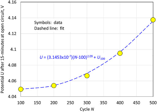
We close this section with an empirical modification of Eqs 65, 66. Above 3.75 V is where the influence of cation-mixing on the voltage trace is most evident and the voltage traces for the different cycles diverge. This is the region that is most sensitive to the value of $\alpha \chi \tau$ as it appears in Eq. 66. It can be seen in Figure 2 and Figure 4 that the rate of increase in the potential at the end of charge in non-linear; i.e., there is less change in the potential at the end of the charge in going from cycle 100 to 200 then in going from cycle 400 to 500. We can estimate the open-circuit potential at the end of charge by plotting the potential after 15 min of open circuit for the data of Figure 2, corresponding to the plot in Figure 5. From Figure 2, we see that after the initiation of charge, the potential immediately jumps to about 3.6 V, after which it transitions smoothly to the end of charge potential; because the charge currents are low (about C/10), the measured cell potential during charge is close to that of the open-circuit potential $U$ . If we approximate the smooth transition to represent a linear potential vs. capacity $U\left(Q\right)$ relation, then we would expect the capacity $Q$ to vary in a quadratic manner with cycle life, reflecting the behavior of $U$ in Figure 5. For small values of $\alpha \chi \tau$ , we can obtain the following from Eq. 66:

${\lim }_{\alpha \chi \tau \to 0}Q\left(\tau \right)=Q_0\left[1-{\overline{x}}_{TM}\left(0\right)\right]\left[1-\alpha \tau \overline{x}\left(0\right)\right],(74)$

which shows that $Q$ declines linearly with time for small values of $\alpha \chi \tau$ . To make $Q$ vary nonlinearly in time for small $\alpha \chi \tau$ , we replace $\alpha$ in Eq. 64 with $\alpha n{t}^{n-1}$ , with $n$ being an additional parameter to be fit to the data, which is equivalent to replacing $\alpha \chi \tau$ in Eq. 66 with $\alpha \chi {\tau }^n$ :

$\begin{array}{c}Q\left(\tau \right)=Q_0\chi \left(\frac{1-{\overline{x}}_{TM}\left(0\right)}{1-{\overline{x}}_{TM}\left(0\right)-\overline{x}\left(0\right)e^{-\alpha \chi {\tau }^n}}\right)+O\left({\alpha }^2{\tau }^n\right)\text{ ,}\\ =FL{\epsilon }_1{\epsilon }_{1F}{c}_T\chi \left(\frac{1-{\overline{x}}_{TM}\left(0\right)}{1-{\overline{x}}_{TM}\left(0\right)-\overline{x}\left(0\right)e^{-\alpha \chi {\tau }^n}}\right)+O\left({\alpha }^2{\tau }^n\right).\end{array}(75)$

In addition, Eq. 65 is replaced by

$\overline{x}\left(\tau \right)=\frac{\overline{x}\left(0\right)\chi e^{-\alpha \chi {\tau }^n}}{1-{\overline{x}}_{TM}\left(0\right)-\overline{x}\left(0\right)e^{-\alpha \chi {\tau }^n}}+O\left({\alpha }^2\tau \right)\text{ and }{\overline{x}}_{TM}\left(\tau \right)=\overline{x}\left(0\right)+{\overline{x}}_{TM}\left(0\right)-\overline{x}\left(\tau \right).(76)$

Consistent with the plot shown in Figure 5, we take $n=2$ as an initial guess for the data fitting process (cf. Table 1).

A more detailed model of the cation-mixing reaction rate (12) would require forward and backward rate constants, reactions between all four galleries (J = 4 for the MSRM as applied to NMC622, cf. Table 2) with all of the transition metals (Ni, Mn, and Co), and the use of activities instead of concentrations for all reactants and products, but this is beyond the scope of this work, and the more detailed approach would require many more unknown parameters. Hence, for this work, the semi-empirical relations (75) and (76) are employed.

TABLE 2

TABLE 2. Thermodynamic parameters and properties used in the simulations. The initial values are from the work of Verbrugge et al. (2017). Note that $X_4=1-X_1-X_2-X_3$ .

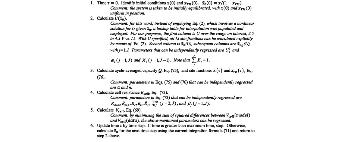
The algorithm used to simulate the data is presented in Table 3.

TABLE 3

TABLE 3. Summary of the algorithm used for the model calculations.

Discussion

For modeling the experimental data, we use the 10-h charge data except for the first 10 min of charge, as the perturbation solution is valid only when the concentration profiles have reached their fully developed state. For the same reason, immediately after the charge current is set to zero for the open-circuit hold, the perturbation solution is not valid; hence, for this work, we used only the last five data points of the open-circuit hold, which are called out in Figure 7, for parameter regression. The sum of the squared differences between the data and the model cell voltages, often termed the sum of squared residuals (Eubank, 1999), was minimized by regressing the parameters as mentioned in the algorithm in Table 3. ³ The sum of squared residuals for the last five data points were multiplied by a factor such that, at the beginning of the regression, the sum of the weighted squared residuals for the last five data points was the same as the sum of squared residuals for the charge portion of the data used in the regression. Initial guesses and regressed values for the parameters are provided in Tables 1, 2, 4, and Table 5. Many of the parameters in Table 1 and Table 4 were used to calculate the resistances showing in Table 5; such parameters show no entry in the column titled “Regressed Value,” as the resistances of Table 5 were used in the regression, consistent with the cell resistance expression, Eq. 73. The first seven resistances listed in Table 5 cannot be regressed separately, as they are all housed in $R_{ohmic}$ (see Eq. 73) and are constants. Initial guesses were employed for all of the first seven resistances, using the values provided in Table 1 and Table 4, and then Eq. 73 was used to calculate the initial guess for $R_{ohmic}$ . For the regression, only $R_{ohmic}$ , $R_k$ , $R_d$ , and ${\widehat{R}}_{Li,f}$ were regressed, with the latter two resistances regressed to zero, implying no measurable Li diffusion resistance within the NMC622 and no measurable resistance growth with time at the Li electrode surface for the low-rate charge operation. Lastly, we only fit the data for cycles 100 and 500. The agreement with all of the data, with exception of the duration immediately after the step to open-circuit where the perturbation solution is not valid, is quantitative insofar as the differences between the data and the calculations are similar to experiment-to-experiment variation.

FIGURE 7

FIGURE 7. Experimental results (symbols) and calculations. The inset plot in the lower right shows only the calculations.

TABLE 4

TABLE 4. Parameters and properties used in the simulations and which are represented by a Greek letter.

TABLE 5

TABLE 5. Initial and regressed sheet resistances. See Eq. 73 for the cell resistance expression.

A comparison of the experimental results with the model calculations using regressed parameters is shown in Figure 7. It is difficult as plotted to see the model calculations, as they are under the symbols for the experimental data as plotted. The inset graphic shows the model calculations during charge. As mentioned previously and discussed in (Baker and Verbrugge, 2021), the perturbation solution assumes diffusion profiles in the solid state that are fully developed, which in turn requires the current to change smoothly (on a time scale of $\tau =t/t_0$ ), and the discontinuities in current that occur at the start of charge and 10 h later, at the start of open circuit, do not satisfy this assumption. As a result, Eq. 69 is inaccurate for a certain period of time after each discontinuity. This is particularly noticeable at the start of the open circuit, when Eq. 69 predicts that the cell voltage is equal to the open-circuit voltage. Instead, a period of time is needed for the diffusion profiles to relax to a steady state (See the data just after 10 h in Figure 4.). The original value for the characteristic diffusion time in the particles is $a^2/D$ = 31 min, longer than the entire 15 min at the open circuit. However, $R_d$ is regressed to zero, implying no measurable diffusion resistance and that $a^2/D$ is less than 31 min; hence, it is likely appropriate to retain the last five data points of the open circuit in the model–experiment comparison.

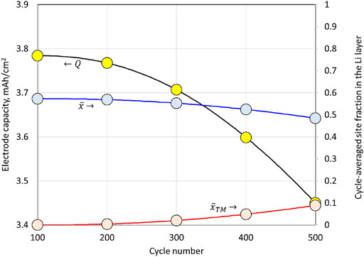
The decline in the calculated cell capacity, which is set by the NMC622 electrode capacity, from cycle $N_0=100$ to cycle 500, is depicted in Figure 8. The decline is slow on a per cycle basis because ${\alpha }^2{\tau }^n<<1$ , consistent with the derivation of Eq. 75, and it is nearly quadratic. The decline in capacity is directly related to the increase in transition metal species in the Li layer. Cycle-averaged site fractions within the Li layer of Li-filled sites $\overline{x}\left(\tau \right)$ and of transition metal filled sites ${\overline{x}}_{TM}\left(\tau \right)$ are also plotted in Figure 8 (cf. Eq. 76).

FIGURE 8

FIGURE 8. Calculated electrode capacity, Eq. 75, and cycle-average site fractions, cf. Eq. 76. The symbols refer to the calculations presented in Figure 7.

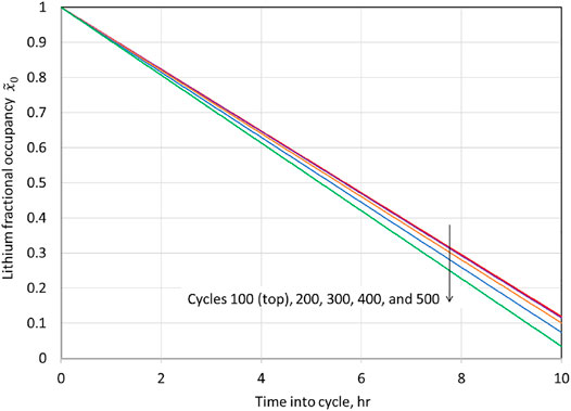
While the perturbation solution (69) is accurate to $O\left({\gamma }^2\right)$ , the resistance Formula (70) needs only the leading order term in $\tilde{x}$ , referred to as ${\tilde{x}}_0$ , for the resistance terms involving $R_k$ and $R_d$ ; ${\tilde{x}}_0$ is the leading order term for the fractional site occupancy of Li in the Li layer of NMC622, and it is uniform throughout the electrode and particles (time dependent but no position dependence). Hence, ${\tilde{x}}_0$ can be deduced once the cell current and Coulombic capacity are known per Eq. 71, in addition to the initial condition ${\tilde{x}}_0\left(0\right)$ . A plot of ${\tilde{x}}_0$ during cell charging is provided in Figure 9. The charge begins with a fully lithiated NMC622, and, with each cycle, the end of the charge value for ${\tilde{x}}_0$ declines due to a loss of capacity. 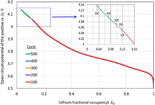Once ${\tilde{x}}_0$ is known, $U\left({\tilde{x}}_0\right)$ is uniquely determined from Eq. 2, with ${\tilde{x}}_0$ replacing $x$ ; i.e., ${\tilde{x}}_0={\displaystyle \sum _j\frac{X_j}{1+\exp \left[f\left(U-U_j^0\right)/{\omega }_j\right]}}$ . A plot of $U\left({\tilde{x}}_0\right)$ for charge during various cycles is shown in Figure 10. The reduced capacity due to cation-mixing leads to higher voltages at the end of the charge, and the nonlinear increase in the end-of-charge open-circuit potential is clear.

FIGURE 9

FIGURE 9. Calculated leading-order term ${\tilde{x}}_0\left(t\right)$ , see Eq. 68, for the fractional occupancy of Li in the Li layer of the NMC622 during various cycles.

FIGURE 10

FIGURE 10. Calculated open-circuit potential vs. the fractional occupancy of Li in the Li layer for various cycles. A blow-up of the potential at the end of de-lithiation is shown in the upper right inset plot.

While one can draw some insight from the regressed parameters, we did not use the perturbation solution and the parameter regression scheme to measure parameters displayed in Table 1 and Table 4 other than those parameters necessary to model the cation-mixing reaction of Eqs 10, 75, 76 for calculations. By using the perturbation solution (69) and the parameter regression scheme, we 1) obtain the open-circuit parameters (Table 2) and 2) we remove an irreversible phenomena associated with the transport and kinetics from the measured cell voltage, enabling us to focus on the degradation of NMC622 via cation-mixing. If we were to seek an accurate measurement of the parameters governing irreversible transport phenomena and kinetics, higher current densities would be needed. As an example of this, in (Baker and Verbrugge, 2018; Baker et al., 2019) low-frequency voltammetry was employed to deduce thermodynamic parameters, and complementary high-frequency voltammetry to gain sensitivity for the measurement of parameters governing irreversible transport phenomena and kinetics. The increase in $R_{Ohmic}$ from the initial estimate of 10 Ω-cm² to the regressed value of 27 Ω-cm² is likely due to a resistive layer over the Li counter electrode surface that remains constant over cycles 100 to 500, corresponding to ${\widehat{R}}_{Li,f,init}$ . ${\widehat{R}}_{Li,f,init}$ was initially set to zero (cf. Table 5) and ${\widehat{R}}_{Li,f,init}$ would correspond to 17 Ω-cm² if ${\widehat{R}}_{Li,f,init}$ were the cause of the increase in $R_{Ohmic}$ .

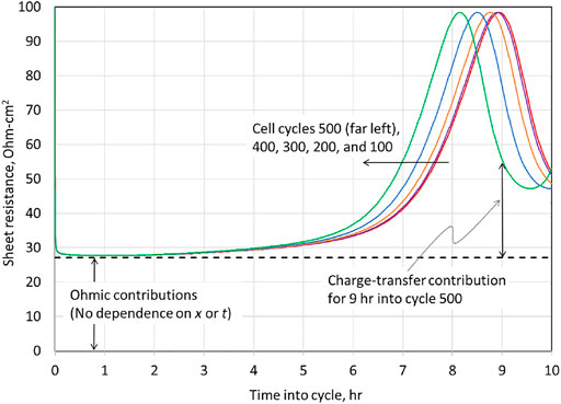
The total cell resistance $R_{cell}$ , Eq. 73, is plotted for various charge cycles in Figure 11. For all cycles, throughout the first half of the charge, $R_{Ohmic}$ dominates the cell resistance. While we incorporated the time-dependent resistance ${\widehat{R}}_{Li,f}\tau$ in Eq. 73 for the growth of a resistive film over the Li surface, cf. Eq. 9, the regressed value for ${\widehat{R}}_{Li,f}$ was zero. Similarly, the resistance to Li diffusion $R_d$ in the NMC622 was regressed to zero. Hence, for the slow (10-h) charges and the ensuing open-circuit stand, we can only detect Ohmic and charge-transfer resistance at the NMC electrode. All resistance above the dashed line in Figure 11 is associated with charge–transfer resistance, $\frac{R_k}{{\displaystyle \sum _{j=1}^J{\overline{i}}_{0,j}^{ref}{\left({\tilde{x}}_{j,0}\right)}^{{\omega }_j{\beta }_j}{(X_j-{\tilde{x}}_{j,0})}^{{\omega }_j(1-{\beta }_j)}}}$ (see Eq. 70), which dominates the total cell resistance for the second half of charge. As mentioned previously, if a more accurate measurement of charge–transfer resistance were desired, higher currents should be investigated.

FIGURE 11

FIGURE 11. Regressed cell resistance (cf. Eq. 73). Ohmic contributions (see $R_{ohmic}$ defined in Eq. 73) dominate for the first half of the charge (0–5 h), after which the charge–transfer resistance $\frac{R_k}{{\displaystyle \sum _{j=1}^J{\overline{i}}_{0,j}^{ref}{\left({\tilde{x}}_{j,0}\right)}^{{\omega }_j{\beta }_j}{(X_j-{\tilde{x}}_{j,0})}^{{\omega }_j(1-{\beta }_j)}}}$ plays an important role.

Summary and Conclusion

We begin this publication with a brief review of the Li metal electrode in non-aqueous solvents and cation-mixing in layered transition metal oxides. Mathematical equations describing these phenomena are then presented as an addition to the equations describing a porous insertion electrode and an adjacent separator (Baker and Verbrugge, 2021). We show that because the degradation associated with cation-mixing is slow, we can average the degradation reaction over each cycle, leading to Eq. 75. The perturbation procedure presented in (Baker and Verbrugge, 2021) is used to derive Eqs 69–72, which constitute our perturbation solution. Equations 66,69–72 simplify significantly the regression of model parameters through the minimization of the sum of squared differences between experimental data and model calculations, as compared to the full numerical solution of Eqs 35–50 embedded within the parameter regression scheme. The good agreement between the perturbation solution and the experimental data (cf. Figure 7) supports the conclusion that cation-mixing is the dominant mechanism for capacity loss in these Li||Ni_0.6Mn_0.2Co_0.2O₂ cells. In summary, the overall procedure of using the low-rate perturbation solution of (Baker and Verbrugge, 2021), along with low-rate data, and averaging degradation reactions over cycles for low rates of degradation, analogous to Eq. 75, can be employed to examine other electrode systems and degradation mechanisms when both are governed by low rates.

Data Availability Statement

The original contributions presented in the study are included in the article/Supplementary Materials; further inquiries can be directed to the corresponding author.

Author Contributions

All authors listed have made a substantial, direct, and intellectual contribution to the work and approved it for publication.

Conflict of Interest

MV, DB, SC, MH, and MC were employed by the company General Motors Research and Development.

Publisher’s Note

All claims expressed in this article are solely those of the authors and do not necessarily represent those of their affiliated organizations, or those of the publisher, the editors, and the reviewers. Any product that may be evaluated in this article, or claim that may be made by its manufacturer, is not guaranteed or endorsed by the publisher.

Footnotes

¹ Because a Li reference electrode is used to determine the potential Φ₂, the salt concentration does not show in the exchange current density in Eq. 4. The discussion in Bizeray et al. [35] in the section “Thermodynamics of reference electrodes” provides helpful commentary on this topic.

² Our interest is the limiting case when $t_0$ tends to infinity. In this limit, the dimensionless parameters $\gamma ,\tilde{\gamma }$ tend to zero, and a perturbation analysis is done for $\gamma ,\tilde{\gamma }<<1$ . However, as $t_0\to \infty$ the ratio $\tilde{\gamma }/\gamma$ remains fixed. Generally speaking, $\tilde{\gamma }/\gamma$ is a very small number, so that terms involving $\tilde{\gamma }$ will also be small if $\gamma$ is small.

³ The Generalized Reduced Gradient (GRG2) Algorithm as implemented in Microsoft Excel was employed to regress the parameters. For history on this Solver, see References [37] and [38].

References

Abdellahi, A., Urban, A., Dacek, S., and Ceder, G. (2016). Understanding the Effect of Cation Disorder on the Voltage Profile of Lithium Transition-Metal Oxides. Chem. Mat. 28, 5373–5383. doi:10.1021/acs.chemmater.6b01438

CrossRef Full Text | Google Scholar

Baker, D. R., and Verbrugge, M. W. (2018). J. Electrochem. Soc. 165, A3952.

CrossRef Full Text

Baker, D. R., Verbrugge, M. W., and Gu, W. (2019). Multi-Species, Multi-Reaction Model for Porous Intercalation Electrodes: Part II. Model-Experiment Comparisons for Linear-Sweep Voltammetry of Spinel Lithium Manganese Oxide Electrodes. J. Electrochem. Soc. 166, A521–A531. doi:10.1149/2.0091904jes

CrossRef Full Text | Google Scholar

Baker, D. R., and Verbrugge, M. W. (2012). Intercalate Diffusion in Multiphase Electrode Materials and Application to Lithiated Graphite. J. Electrochem. Soc. 159, A1341–A1350. doi:10.1149/2.002208jes

CrossRef Full Text | Google Scholar

Baker, D. R., and Verbrugge, M. W. (2021). Slow Current or Potential Scanning of Battery Porous Electrodes: Generalized Perturbation Solution and the Merits of Sinusoidal Current Cycling. J. Electrochem. Soc. 168, 050526. doi:10.1149/1945-7111/abf5f5

CrossRef Full Text | Google Scholar

Bizeray, A. M., Howey, D. A., and Monroe, C. W. (2016). Resolving a Discrepancy in Diffusion Potentials, with a Case Study for Li-Ion Batteries. J. Electrochem. Soc. 163, E223–E229. doi:10.1149/2.0451608jes

CrossRef Full Text | Google Scholar

Chen, S. (2018). Adv. Mat. 30, 1706102. doi:10.1002/adma.201706102)

CrossRef Full Text

Cheng, X.-B., Zhang, R., Zhao, C.-Z., and Zhang, Q. (2017). Toward Safe Lithium Metal Anode in Rechargeable Batteries: A Review. Chem. Rev. 117, 10403–10473. doi:10.1021/acs.chemrev.7b00115

PubMed Abstract | CrossRef Full Text | Google Scholar

Eijima, S., Sonoki, H., Matsumoto, M., Taminato, S., Mori, D., and Imanishi, N. (2019). Solid Electrolyte Interphase Film on Lithium Metal Anode in Mixed-Salt System. J. Electrochem. Soc. 166, A5421–A5429. doi:10.1149/2.0611903jes

CrossRef Full Text | Google Scholar

Eubank, R. L. (1999). Nonparametric Regression and Spline Smoothing. 2nd edition. Boca Raton, FL: CRC Press.

Google Scholar

Fang, C. (2021). Nat. Energy 6, 987.

Fylstra, D., Lasdon, L., Watson, J., and Waren, A. (1998). Design and Use of the Microsoft Excel Solver. Interfaces 28, 29–55. doi:10.1287/inte.28.5.29

CrossRef Full Text | Google Scholar

Guggenheim, E. A. (1977). Thermodynamics. 6th ed. Amsterdam: North-Holland.

Google Scholar

Hobold, G. M., Lopez, J., Guo, R., Minafra, N., Banerjee, A., Shirley Meng, Y., et al. (2021). Moving beyond 99.9% Coulombic Efficiency for Lithium Anodes in Liquid Electrolytes. Nat. Energy 6, 951–960. doi:10.1038/s41560-021-00910-w

CrossRef Full Text | Google Scholar

Julien, C., Mauger, A., Zaghib, K., and Groult, H. (2016). Optimization of Layered Cathode Materials for Lithium-Ion Batteries. Materials 9, 595. doi:10.3390/ma9070595

PubMed Abstract | CrossRef Full Text | Google Scholar

Kim, N. Y., Yim, T., Song, J. H., Yu, J.-S., and Lee, Z. (2016). Microstructural Study on Degradation Mechanism of Layered LiNi0.6Co0.2Mn0.2O2 Cathode Materials by Analytical Transmission Electron Microscopy. J. Power Sources 307, 641–648. doi:10.1016/j.jpowsour.2016.01.023

CrossRef Full Text | Google Scholar

Kim, N. Y., Yim, T., Song, J. H., Yu, J.-S., and Lee, Z. (2016). Microstructural Study on Degradation Mechanism of Layered LiNi0.6Co0.2Mn0.2O2 Cathode Materials by Analytical Transmission Electron Microscopy. J. Power Sources 307, 641–648. doi:10.1016/j.jpowsour.2016.01.023

CrossRef Full Text | Google Scholar

Lasdon, L. S., Waren, A. D., Jain, A., and Ratner, M. (1978). “Design and Testing of a Generalized Reduced Gradient Code for Nonlinear Programming,”. ACM Trans. Math. Softw. 4 (No. 1), 34–49. doi:10.1145/355769.355773

CrossRef Full Text | Google Scholar

Li, H., Li, J., Ma, X., and Dahn, J. R. (2018). J. Electrochem. Soc. 165, A1038. doi:10.1149/2.0861805jes

CrossRef Full Text

Li, H., Li, J., Ma, X., and Dahn, J. R. (2018). J. Electrochem. Soc. 165, A1038. doi:10.1149/2.0861805jes

CrossRef Full Text

Liao, P. Y., Duh, J. G., and Sheen, S. R. (2005). Effect of Mn Content on the Microstructure and Electrochemical Performance of LiNi[sub 0.75−x]Co[sub 0.25]Mn[sub x]O[sub 2] Cathode Materials. J. Electrochem. Soc. 152, A1695. doi:10.1149/1.1952687

CrossRef Full Text | Google Scholar

Liu, B., 1 J-Zhang, G., and Xu, W. (2018). Advancing Lithium Metal Batteries. Joule. doi:10.1016/j.joule.2018.03.008

CrossRef Full Text | Google Scholar

Meibuhr, S. G. (1970). Electrode Studies in Nonaqueous Electrolytes. J. Electrochem. Soc. 117, 56. doi:10.1149/1.2407438

CrossRef Full Text | Google Scholar

Niu, C. (2021). Nat. Energy 6, 723.

NohNoh, H.-J., Youn, S., Yoon, C. S., and Sun, Y.-K. (2013). Comparison of the Structural and Electrochemical Properties of Layered Li[NixCoyMnz]O2 (X = 1/3, 0.5, 0.6, 0.7, 0.8 and 0.85) Cathode Material for Lithium-Ion Batteries. J. Power Sources 233, 121–130. doi:10.1016/j.jpowsour.2013.01.063

CrossRef Full Text | Google Scholar

Ohzuku, T., Ueda, A., Nagayama, M., Iwakoshi, Y., and Komori, H. (1993). Comparative Study of LiCoO2, LiNi12Co12O2 and LiNiO2 for 4 Volt Secondary Lithium Cells. Electrochimica Acta 38, 1159–1167. doi:10.1016/0013-4686(93)80046-3

CrossRef Full Text | Google Scholar

Peled, E. (1979). J. Electrochem. Soc. 126, 2047.

CrossRef Full Text

Peled, E., and Menkin, S. (2017). Review-SEI: Past, Present and Future. J. Electrochem. Soc. 164, A1703–A1719. doi:10.1149/2.1441707jes

CrossRef Full Text | Google Scholar

Rossen, E., Reimers, J., and Dahn, J. (1993). Synthesis and Electrochemistry of Spinel LT-LiCoO2. Solid State Ionics 62, 53–60. doi:10.1016/0167-2738(93)90251-w

CrossRef Full Text | Google Scholar

Rossen, E., Reimers, J., and Dahn, J. (1993). Synthesis and Electrochemistry of Spinel LT-LiCoO2. Solid State Ionics 62, 53–60. doi:10.1016/0167-2738(93)90251-w

CrossRef Full Text | Google Scholar

Schipper, F., Erickson, E. M., Erk, C., ShinShin, J.-Y., Chesneau, F. F., and Aurbach, D. (2017). Review-Recent Advances and Remaining Challenges for Lithium Ion Battery Cathodes. J. Electrochem. Soc. 164, A6220–A6228. doi:10.1149/2.0351701jes

CrossRef Full Text | Google Scholar

Usubelli, C. (2020). J. Electrochem. Soc. 167, 080514.

CrossRef Full Text

Verbrugge, M., Baker, D., Koch, B., Xiao, X., and Gu, W. (2017). Thermodynamic Model for Substitutional Materials: Application to Lithiated Graphite, Spinel Manganese Oxide, Iron Phosphate, and Layered Nickel-Manganese-Cobalt Oxide. J. Electrochem. Soc. 164, E3243–E3253. doi:10.1149/2.0341708jes

CrossRef Full Text | Google Scholar

Verbrugge, M. W., and Koch, B. J. (1994). J. Electrochem. Soc. 141, 3053.

CrossRef Full Text

Xue, W. (2020). Energy Environ. Sci. 13, 212.

Google Scholar

Y-Choi, M., S-Pyun, I., and S-Moon, I. (1996). Solid State Ionics 89, 43.

Zheng, J. (2019). Acc. Chem. Res. 52, 2201. doi:10.1021/acs.accounts.9b00033

PubMed Abstract | CrossRef Full Text

Zhu, P., Seifert, H. J., and Pfleging, W. (2019). The Ultrafast Laser Ablation of Li(Ni0.6Mn0.2Co0.2)O2 Electrodes with High Mass Loading. Appl. Sci. 9, 4067. doi:10.3390/app9194067

CrossRef Full Text | Google Scholar

Nomenclature

$a$ Spherical particle radius in a porous electrode, cm

$a_s=\frac{3{\epsilon }_1}{a}$ Surface to volume ratio of a porous electrode, 1/cm

$c_0$ Value of $c_2$ at equilibrium, mol/cm³

$c_2$ Salt concentration in the liquid phase, mol/cm³

$c_f$ Film concentration, Eq. 9, mol/cm³

$c_T$ Total Li site concentration in the Li layer of the NMC622, mol/cm³

$D$ Diffusion coefficient of Li-filled sites in the Li layer, cm²/s

$D_2$ Salt diffusion coefficient in the liquid phase, cm²/s

$f=\frac{F}{RT}$ V^-1

$f_{\pm }$ Activity coefficient of electrolyte salt

$F$ Faraday’s constant, C/mol

$i,i_j$ Total current density, current density of species j, A/cm²

$i_{0,j}$ Exchange current densities, A/cm²

$j$ Current density of lithium insertion into the NMC622 phase

$L,L_2$ Width of porous electrode or separator, cm

$n$ See Eq. 75

$N,N_H$ Flux of the occupied sites or vacancies in lithium host, mol/cm²-s

$Q_0$ Total capacity per geometric area of electrode, C/cm²

$Q$ $Q_0(1-{\overline{x}}_{TM})$ , C/cm²

$r$ Radial coordinate in spherical particles, cm (See Figure 6)

$r_{CM}$ Rate of cation mixing, Eq. 12 mol/cm³-s

$r_f$ Rate of Li consumption for film formation, Eq. 9, mol/cm³

$R$ Gas constant, J/cm³-K

$\begin{array}{l}{R}_c,R_e,R_s,R_{e,diff},\\ R_{sep},R_d,R_k,R_f,\\ R_{k,Li},{\widehat{R}}_{Li,f,init},{\widehat{R}}_{Li,f}\end{array}$ Sheet resistances, Eq. 33, Ohm-cm²

$t$ Time, s

$t_0$ Total cycle time, s

$t_{+}^0$ Lithium ion transference number

$T$ Temperature, K

$U$ Open circuit voltage, V

$U_j,U_j^0$ See Eq. 2, V

$V_{cell}$ Cell voltage, V

$x$ Total mole fraction of Li in the Li layer of NMC622

$\tilde{x}$ $=\frac{x}{\left(1-x_{TM}\right)}$

$x_j,x_{H,j},X_j$ See Eq. 2

$x_{TM}$ Fraction of Li sites in the NMC622 filled with transition metals, Eq. 11

$X_{TM}$ Fraction of TM sites filled with a transition metal

$z$ Coordinate in the porous electrode, cm (See Figure 6)

$\alpha$ See Eq. 34

${\beta }_j$ Symmetry factor

$\gamma ,\tilde{\gamma }$ See Eq. 34

${\Gamma }_1,{\Gamma }_{2,E},{\Gamma }_{2,S}$ Tortuosity for the solid and liquid phases in the electrode or separator

${\epsilon }_1,{\epsilon }_2$ Porosity of the solid or liquid phase

${\epsilon }_{1,F}$ Fraction of the solid phase that is active material

${\eta }_s$ Surface overpotential

${\kappa }_1,{\kappa }_2$ Conductivity in the solid or liquid phase, S/cm

$\widehat{\kappa }$ See Eq. 34

$\mu$ Chemical potential of Li filled sites in the Li layer of NMC622, Eq. 17

${\Phi }_1,{\Phi }_2$ Potential in the solid (1) or liquid (2) phase, V

$\tau =\frac{t}{t_0}$ Dimensionless time

${\tau }_1,{\tau }_{2,E},{\tau }_{2,S}$ Tortuosity, solid (1), electrode liquid phase $\left(2,E\right)$ , separator $\left(2,S\right)$

${\omega }_j$ See Eq. 2