 Fangze Wu
 Mao Yang
 Chaoyu Shi
- Key Laboratory of Modern Power System Simulation and Control & Renewable Energy Technology, Ministry of Education, Northeast Electric Power University, Jilin, China
As the wind power penetration increases, the short-term prediction accuracy of wind power is of great importance for the safe and cost-effective operation of the power grid in which the wind power is integrated. Traditional wind farm power prediction uses numerical weather prediction (NWP) information as an important input but does not consider the correlation characteristics of NWP information from different wind farms. In this study, a convolutional neural network–long short-term memory based short-term prediction model for wind farm clusters is proposed. Additionally, a feature map is established for multiposition NWP information, the spatial correlation of NWP information from different wind farms is fully explored, and the feature map is trained using the spatiotemporal model to obtain the short-term prediction results of wind farm clusters. Finally, as a case study, the operational data of a wind farm cluster in China are analyzed, and the proposed model outperforms traditional short-term prediction methods in terms of prediction accuracy.
1 Introduction
In recent years, as its installed capacity continuously increases, the fluctuation and randomness of wind power have made the scheduling and reliability control of power systems more difficult. Accurate day-ahead wind-power forecasts can help to reduce the impact of wind-power integration on power systems, as well as facilitate the scheduling department to formulate efficient, feasible daily power generation plans and adjust the reserve capacity of systems (Wang et al., 2018a). Thus, accurate wind-power forecasts are important for determining reasonable scheduling plans and ensuring the safe, economic operation of power grids (Yang and Huang, 2018).
Currently, the main wind-power forecasting methods include physical, statistical, learning, and combination methods. Physical methods forecast wind speeds using numerical weather prediction (NWP) models based on the information (e.g., contour lines, roughness, obstacles, pressure, and temperature) about the surroundings of wind farms (WFs). Generally, results produced by physical methods are used as the input for other statistical models or to forecast the power of newly constructed WFs. Statistical and learning methods generally do not consider the physical process of wind-speed changes but instead forecast the output power of WFs by mapping it to historical statistical data. As their forecasting accuracies decrease as the length of the forecasting period increases, these methods are predominantly employed in short-term forecasting. Common statistical and learning methods include the Kalman filter, artificial neural networks (Wu and Feng, 2018), wavelet decomposition (Safari et al., 2018), support-vector machines (SVMs) (Zendehboudi et al., 2018), probabilistic forecasting (Xu et al., 2019), and chaotic forecasting (Hong et al., 2019). By using the information provided by different models and exploiting their respective advantages, a combination method combines these models into one forecasting model based on a suitable weighted averaging scheme (Vluymans et al., 2019). Common combinations include those of physical and statistical methods, those of short- and mid-term forecasting models, and those of statistical models. Compared to those produced by single models, wind-power forecasts produced by combined models have fewer relatively large errors and, as a result, higher accuracies (Zhou et al., 2019).
Yang et al. (Yang et al., 2021) proposed A day ahead wind power prediction model based on equivalent power curve clustering is proposed. Turbines with similar power output characteristics are divided into several categories by using the improved FCM method, and the power curve with representative examples is selected as the equivalent curve of the wind farm, to capture the performance of the wind turbine and effectively improve the prediction accuracy. The power fluctuation between the wind farm and wind farm cluster have been analyzed (Yang et al., 2020). In view of the changes in the status of WFs, Daniel and Fang (Tabas et al., 2019) evaluated the operating conditions of wind turbines using random matrix theory while considering wind-resource data and, on this basis, constructed a dynamic forecasting model to further improve the forecasting accuracy. Zhang (Zhang et al., 2020) clustered wind power into different groups based on the fluctuation process, extracted the characteristic curves of different fluctuations, comprehensively considered wind-power fluctuations, and, on this basis, put forward an error correction model. Wang et al. (Wang et al., 2018b) performed a multi-classification operation on time-series power sample sets with similar features based on distance and form trend using the multi- and hierarchical clustering methods to determine the time-series features of the data, to improve the forecasting accuracy.
Owing to the emergence of artificial intelligence (AI) and big data technology, current research on short-term wind-power forecasting is focused on AI-based forecasting. Fan et al. (Fan et al., 2020) proposed a new spatiotemporal neural network composed of a convolutional neural network (CNN) and a bidirectional gated recurrent unit (GRU) to extract the respective spatiotemporal features of historical data (e.g., wind speeds and directions) and NWPs. By integrating the features, they produced wind-speed forecasts. Wu et al. (Wu et al., 2021) put forward a CNN–LSTM-based ultra-short-term wind-power forecasting model to analyze and model some NWP data and historical observation data.
Castellani et al. (Castellani et al., 2016)]compared a pure ANN power forecast with a hybrid method. A new framework for forecasting one-day-ahead wind power generation based on information amalgamation from multiple sources is proposed by Vaccaro et al. (Vaccaro et al., 2011) Zhao et al. (Zhao et al., 2012) presents the performance evaluation and accuracy improvement of a novel day-ahead wind power forecasting system in China. Qin et al. (Qin et al., 2011) established a hybrid optimization algorithm to improve the accuracy of the forecast. Mana et al. (Mana et al., 2020) discussed the different forecast configurations for predicting the future day production of a wind farm located in moderately complex terrain. Miettinen et al. (Miettinen and Holttinen, 2017) studied the day-ahead forecast errors in four Nordic countries as well as the effect of wind farm dispersion on forecast errors in areas of different sizes. Bochenek et al. (Bochenek et al., 2021) investigated the possibility of predicting day-ahead wind power based on different machine learning methods not for specific wind farms but at the national level.
For wind power day-ahead prediction, current studies have constructed suitable models based on the current main research methods for wind power prediction, and the prediction accuracy is improved with the help of artificial intelligence and big data technology.
This paper presents a short-term power forecasting method for WF clusters (WFCs) based on a spatiotemporal neural network. First, a feature map matrix is generated through permutation and combination of the NWP data for all the WFs within a cluster for each moment. Then, features are extracted using the spatiotemporal model. Finally, a short-term power forecast is produced for the WFC. Compared to a cumulative sum of the separate short-term forecasts for all the WFs within a cluster, the proposed method treats the overall power of the WFC as the input, which, to a certain extent, reduces the forecasting error. The method in this paper constructs a feature map based on the NWP information of multiple moments and WFs and builds a dynamic model based on CNN-LSTM architecture on this basis. The method can extract spatio-temporal features and fully consider the correlation among WFs within the WFC.
2 Comparative Analysis of Forecasting for Single Wind Farms and Wind Farm Clusters
Conventional spatiotemporal correlation analysis decomposes spatiotemporal correlations into spatial and temporal correlations. Spatial correlations refer to the certain correlations between wind-power forecasts for different locations at the same time section. Temporal correlations refer to the periodic or aperiodic variations of some attributes of the wind-power forecast for the same spatial point with time.
A WFC located in a large area, consists of many wind farms. The power of the WFC is collectively integrated into the power system. Although the power of a WFC is the sum of the power from all WFs in the cluster, the power fluctuations of a WFC would be different from those of individual WFs.
For a single WF, the values of the meteorological factors (e.g., wind speed and direction) at different heights are relatively strongly correlated due to the action of atmospheric motion within the region. This means that the value of the current variable at a certain forecasting moment is related to both its historical values and the historical values of the factors (e.g., wind speed and direction) at other heights. In comparison, with respect to power forecasting for a WFC, to reduce the accumulation of the forecasting errors for individual WFs generated during the forecasting process, we, in this study, consider the WFC as a whole and put forward a new spatiotemporal correlation analysis method. The information for multiple WFs at different locations is represented by feature maps in the form of time sections. Multi-location, multi-factor time slices are thus formed and subsequently arranged in chronological order.
When analyzing the spatiotemporal correlations of a single WF, a two-dimensional (2D) model is constructed based on the WF data and analyzed using various methods. The extracted correlations are always on a 2D plane. As a result, the spatial correlations of the WF cannot be expressed in their entirety. In contrast, when it comes to the spatiotemporal correlations of a WFC proposed in this study for forecasting, a three-dimensional structure is constructed based on the WFC data, thereby enhancing the spatial structure between the data. In addition, the time-series relations are closely combined at different spatial locations to further explain the meaning of multi-WF, multi-location spatiotemporal correlations. Figure 1 explains the meaning of spatiotemporal correlations for single WFs and WFCs with graph structures.
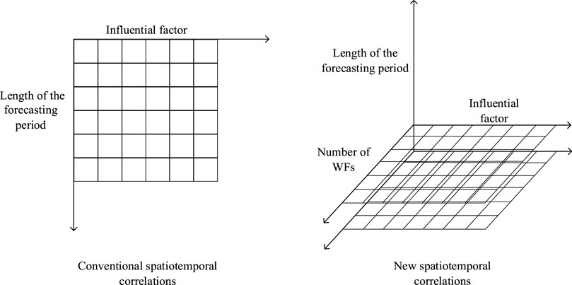
FIGURE 1. Traditional and new spatiotemporal correlation principles.
3 Deep Convolutional Neural Network Modeling Method
3.1 Convolutional Neural Networks
CNNs are a type of typical deep-learning model capable of efficiently identifying features that have emerged in recent years and have become a topical area of research in the image processing field. A CNN has a convolutional deep structure. Weight sharing can suppress overfitting. The local receptive-field design in a CNN is invariant to scaling, translation, and other forms of deformation.
A standard CNN consists generally of an input layer, convolutional layers, pooling layers, fully-connected layers, and an output layer, as shown in Figure 2. A convolutional layer may contain multiple feature maps, each of which is correlated with a convolution kernel. A convolutional layer performs a convolution operation on the local receptive field of the input signal and the convolution kernel and subsequently extracts local features through the activation layer. The input data for a convolutional layer from its preceding layer are a matrix, which, in this study, is composed of the NWP data for multiple units for a period of time. A group of convolution-kernel functions can be defined in a convolutional layer. The feature maps of a convolutional layer are formed by processing the result of the convolution operation on each convolution kernel and the input data plus the bias through the activation function. The convolution process is described as follows:
where
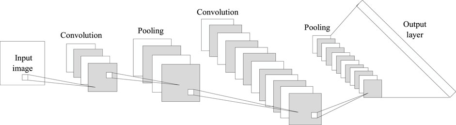
FIGURE 2. Structure of standard convolutional neural network.
Generally, a large number of convolution kernels are used in the convolutional layers to more effectively extract features. As a result, the features obtained by the convolutional layers have a very large number of dimensions, which increases both the computational cost and the likelihood of overfitting. The pooling function in a pooling layer substitutes the overall statistical feature of the output adjacent to a certain location for the output of the network at this location. For example, the max-pooling function gives the maximum value within the adjacent rectangular region. When the input slightly translates, pooling can help to approximately keep the representation of the input unchanged, thereby reducing the feature dimensionality and improving the statistical efficiency of the network.
A pooling layer is usually added after a convolutional layer. This, in fact, is a downsampling operation. Using the overall statistical feature of the region adjacent to a certain location as the output of the network at this location can reduce the dimensionality of the feature maps and the number of parameters of the network while effectively preventing the network from overfitting. The max-pooling equation is as follows:
where
A fully-connected layer classifies, regresses, and identifies signals from which features have been extracted, as well as linearly transforms the input through the activation function and bias, which can be expressed as follows:
where
3.2 Long Short-Term Memory Neural Networks
LSTM is a variant of the recurrent neural network (RNN) architecture. LSTM can effectively address the gradient vanishing and exploding problems encountered during the training of RNNs. As shown in Figure 3, the cell units in an LSTM network comprise gate-control units (including input, output, and forget gates) and memory units.
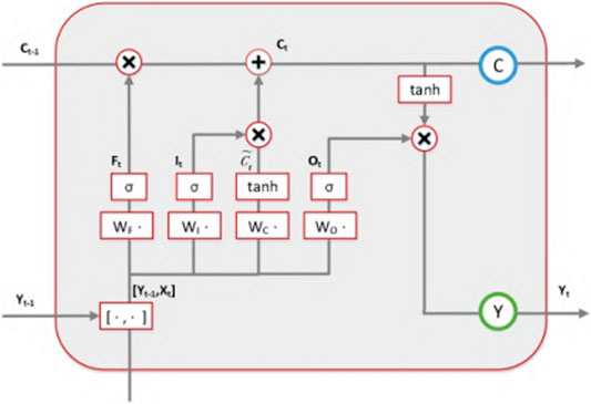
FIGURE 3. Network structure of LSTM unit.
The expression of the forget-gate structure is as follows:
where
In Eqs 5–7,
4 Numerical Weather Prediction and Short-Term Output Forecasting Model for Wind Farms
4.1 Construction of Feature Maps
Extensive research finds that the forecasting accuracy for wind power can be effectively improved by considering the spatiotemporal correlations during the forecasting process. The CNN–LSTM architecture displays certain advantages in processing the time-series relations of high-dimensional data and memory. Figure 4 shows the time-series feature map proposed in this study for the spatial and time-series relations of WFs in a WFC.
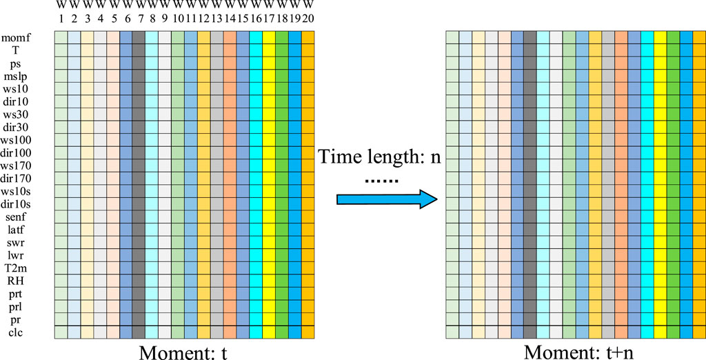
FIGURE 4. Time sequence characteristic diagram.
The NWP data are from the NWP product provided by a Meteorological Centre. The numerical data-set has been validated by comparingthe NWP results with the measured data under the same hub height, the agreement for the whole year is close to 90%.
A spatial feature map is generated by arranging the NWP data for 20 WFs for each moment. Let t and n be the initial moment and the length of the training period, respectively. A feature map rich in spatial structure is formed for each moment. The n number of spatial feature maps forms a time-series feature map. Thus, the rich spatiotemporal correlation information between the WFs is included in the time-series feature map. The NWP data used in this study contain 24 parametric variables. Table 1 summarizes the meaning and name of each parameter. Table 2 summarizes the parameter names of the WFs.
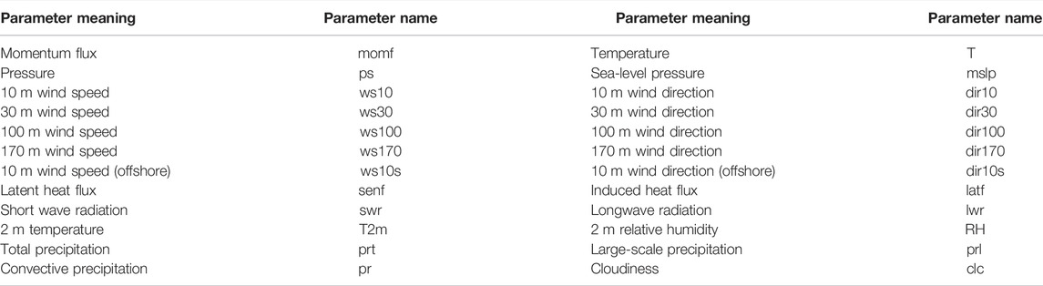
TABLE 1. NWP parameter meaning and name for one wind farm.
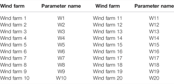
TABLE 2. Parameter names of wind farms.
4.2 Overall Framework/Strategy for Short-Term Wind-Power Forecasting
This study presents a day-ahead power forecasting method for WFCs based on a CNN–LSTM spatiotemporal network model. First, the available WF data are preprocessed. Considering the NWP information for multiple WFs, multi-moment, multi-location NWP information is integrated by constructing feature maps. This way, both the spatial structure and time-series features of the data are preserved. The CNN comprises a feature extraction stage and a classification stage. Multiple filters are constructed to extract the effective features of the input data. The input data are subjected to convolution and pooling operations through the filters. Through continuous extraction and training, output data with space-invariant features are ultimately obtained. The LSTM network continues to preserve the time-series features of the data with spatial features. The CNN–LSTM model is then employed to produce a short-term power forecast for the WFC. Figure 5 shows the short-term WFC power forecasting architecture based on the CNN–LSTM model.
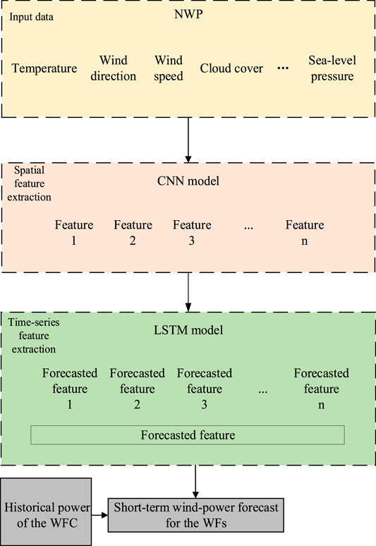
FIGURE 5. Short term prediction flow chart of wind power cluster output based on CNN-LSTM model.
4.3 Convolutional Neural Network–Long Short-Term Memory Model Structure
According to Section 3.1, each feature map is a 24 × 20 order matrix. Each feature map is input into an independent CNN unit. Each network unit consists of two convolutional layers, two pooling layers, and one fully-connected layer. In addition, 3 × 3 convolution kernels are selected for the convolutional layers, and the max-pooling strategy is adopted for the pooling layers. The sampling-pool size is set to 2 × 2. The first layer is a convolution layer, C1, with 50 3 × 3 convolution kernels. The second layer is a pooling layer, C2, with 100 2 × 2 convolution kernels. The third layer is a convolutional layer, C3, with 50 3 × 3 convolution kernels. The fourth layer is a pooling layer, C4, with 200 2 × 2 convolution kernels. The fifth layer is a fully-connected layer, F5, which reconstructs the 2D feature map output by C4 into a 1D vector. By extracting the spatial features between the WFs and reducing dimensionality using the CNN, the feature maps are transformed to a 1D dataset, which is then input into the LSTM model to extract the temporal correlations. Based on the results obtained on multiple simulation training sets, the main parameters of the LSTM model are set as follows: The LSTM model is composed of three network layers with a maximum number of iterations of 180, namely, an LSTM layer that contains one neuron, a dropout layer that contains 17 neurons, and one hidden layer that contains one neuron. The output data corresponding to each moment is input into the subsequent fully-connected layer. Figure 6 shows the CNN–LSTM model structure.
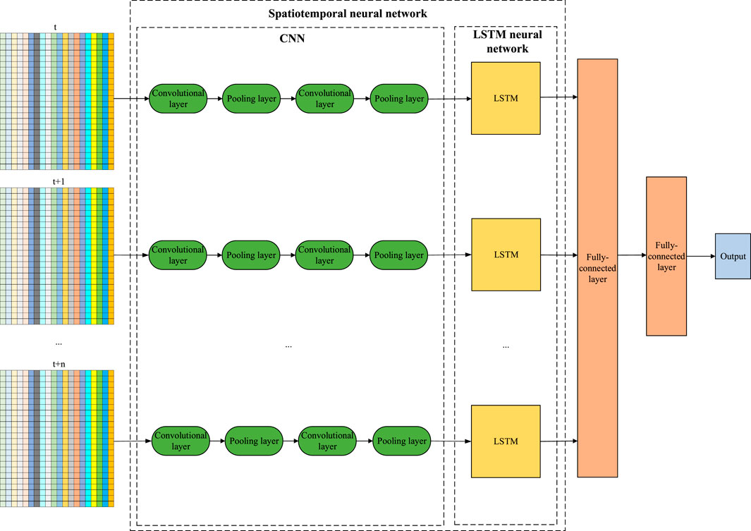
FIGURE 6. CNN-LSTM model structure.
5 Case Study
5.1 Description of the Dataset and Data Preprocessing
The data for a WFC in northeastern China were selected to conduct a case study. The WFC consists of a total of 20 WFs. The geographical span of this WFC is ∼235 km × 330 km. Figure 7 shows the distribution of the WFs. The data for the first 2 months in the dataset for each season of 2018 were selected to form a training set, while the data for the last month were used to form a test set. The time length for each forecast was set to 24 h. The number of times of rolling was set to 30. The data-sampling interval was set to 15 min. All the experiments were performed under the Keras deep-learning framework in Python 3.7. The parameters of the CNN–LSTM model need to be adjusted according to the WF conditions in practice.
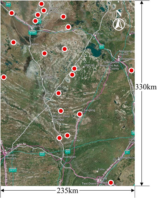
FIGURE 7. Geographic location map of the wind farm cluster.
The NWP-derived features differ in dimension. Therefore, to ensure that the extent of the correlation between each variable and power is equally considered, the NWP data and power need to be subjected to a min-max normalization operation to normalize them to the interval of [0, 1], i.e.,
where
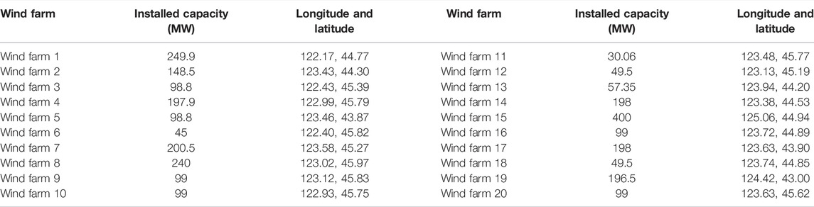
TABLE 3. The installed capacity of wind farms in the case study.
5.2 Evaluation Indices
To accurately evaluate the effectiveness of the proposed forecasting method, two error evaluation indices, namely, fitted mean absolute error (MAE) and root-mean-square error (RMSE), were chosen in this study. They can be calculated using the following equations:
where
5.3 Description of the Comparison Models
The backpropagation (BP) neural network is a common method used to forecast wind power. This method is a multilayered feedforward network capable of learning and storing input-output mapping relations. The radial basis function (RBF) method generates a training model by constructing an RBF. Forecasts can then be produced by inputting relevant future information into the training model. Similarly, the SVM method is a time-series forecasting method capable of reflecting the features of statistical data.
5.4 Results and Analysis
Figure 8 shows the forecasts for the WFC for the 10th day obtained on the test set of each season (i.e., the 10th day obtained on the third month of each season), and compares the actual power of the WFC and the power forecasted by each method. The power forecasted by the proposed method is closer to the actual power. Wind energy fluctuates and is random at different times and in different seasons, making the capture of its pattern of change difficult. The BP, RBF, and SVM methods are unable to satisfactorily track the changes in the wind-power output when it fluctuates significantly. The spatiotemporal model accounts for each meteorological factor affecting the WFC and extracts its features on the same temporal plane, thereby preserving the spatial structure of the data as well as ensuring their time-series features. For the periods with wind-power fluctuations, the forecasts produced by the spatiotemporal model by nonlinear fitting are slightly closer to the actual values than those produced by the other methods. The proposed method yields relatively good forecasts.
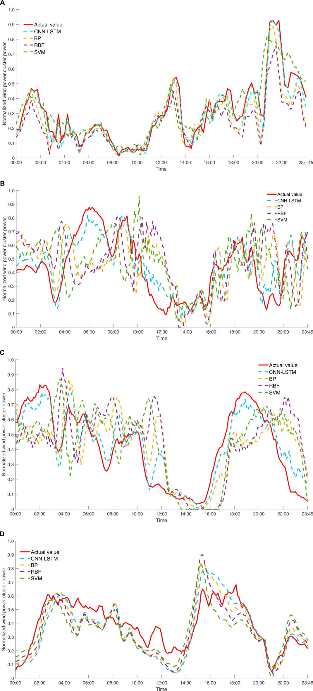
FIGURE 8. Forecast effect of the 10th day of each season in 2018. (A) Spring (B) Summer (C) Fall (D) Winter.
The data in Table 4 show that both the RMSE and MAE of the forecasts produced by the spatiotemporal network model proposed in this study for each season are lower than those of the forecasts produced by the other forecasting models. The forecasting accuracy of each model varies from season to season. The forecasts produced by the spatiotemporal neural network model for the four seasons are relatively stable, with RMSEs of 16.28, 16.17, 17.01, and 16.93% and MAEs of 11.34, 11.81, 12.56, and 12.27%, respectively. The forecasting accuracy of each of the other models varies considerably from season to season, with a difference of approximately 1–5% in both the RMSE and MAE between seasons. Overall, each model exhibits a higher forecasting accuracy for spring and summer than for fall and winter.
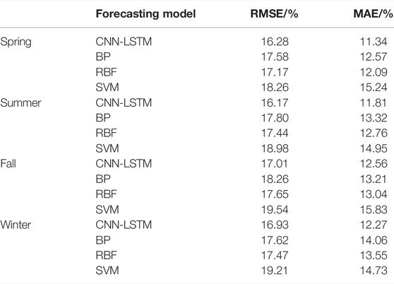
TABLE 4. Comparison of evaluation indexes of the prediction model.
Persistence is a benchmark comparison method that can be used to compare with other methods. It is commonly applied to ultra-short-term forecasting or medium and long-term forecasting. In this paper, for day-ahead forecasting, the wind power fluctuates more rapidly in such a time scale, and the prediction error of the persistence method is significant.
To adequately analyze and examine the reasonableness of the proposed method, the overall power forecasting method for WFCs proposed earlier is denoted by method 1, while a cumulative sum of the individual short-term forecasts for the 20 WFs is denoted by method 2. According to the data in Table 5, for each season, both the RMSE and MAE of the forecast produced by method 1 are lower than those of the forecast produced by method 2. This suggests that the forecasting accuracy of the method that treats the WFC as a whole (i.e., method 1) is higher than that of the method that cumulatively adds the separate forecasts for the WFs (i.e., method 2) and, further, that method 1 effectively avoids an accumulation of errors in the forecasting process.
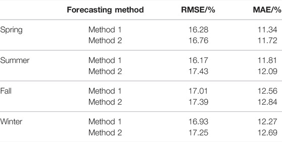
TABLE 5. Accuracy comparison of prediction methods.
6 Conclusion
This paper presents a short-term power foresting method for WFCs that deeply mines the spatiotemporal features. This method constructs feature maps based on multi-moment, multi-WF NWP information and, on this basis, establishes a dynamic model based on the CNN–LSTM architecture. In addition, this method is capable of extracting spatiotemporal features and sufficiently accounts for the correlations between the WFs within a WFC. The following conclusions are obtained from the case study conducted based on the actual operating data for a WFC in northeastern China:
1) Based on the overall trend of the forecasts and the evaluation indices (i.e., RMSE and MSE), the proposed method outperforms the classical methods in forecasting the power of the WFC and has the potential for a wider range of applications.
2) Compared to the cumulative sum of the separate forecasts for single WFs, forecasting the power of the WFC as a whole can effectively avoid an accumulation of forecasting errors.
With the continual increase in the dataset size, a larger number of iterations and a longer time are needed to compute the similarities between data. The linear increase in time complexity poses a challenge to the processing of large datasets.
Data Availability Statement
The original contributions presented in the study are included in the article/Supplementary Material, further inquiries can be directed to the corresponding author.
Author Contributions
FW: Formal analysis, and Writing-Original Draft. MY: Methodology, Writing-Review and Editing and Funding acquisition. CS: Conceptualization, and Writing-Review and Editing.
Funding
This work was financially supported by the National Nature Science Foundation of China (No. 61873091).
Conflict of Interest
The authors declare that the research was conducted in the absence of any commercial or financial relationships that could be construed as a potential conflict of interest.
Publisher’s Note
All claims expressed in this article are solely those of the authors and do not necessarily represent those of their affiliated organizations, or those of the publisher, the editors and the reviewers. Any product that may be evaluated in this article, or claim that may be made by its manufacturer, is not guaranteed or endorsed by the publisher.
References
Bochenek, B., Jurasz, J., Jaczewski, A., Stachura, G., Sekuła, P., Strzyżewski, T., et al. (2021). Day-Ahead Wind Power Forecasting in Poland Based on Numerical Weather Prediction. Energies, 14. 8, 2164. doi:10.3390/en14082164
Castellani, F., Astolfi, D., Mana, M., Burlando, M., Meißner, C., and Piccioni, E. (2016). Wind Power Forecasting Techniques in Complex Terrain: ANN vs. ANN-CFD Hybrid Approach. J. Phys. Conf. Ser. 753 (8), 082002. doi:10.1088/1742-6596/753/8/082002
Fan, H., Zhang, X., Mei, S., Chen, K., and Chen, X. (2020). M2GSNet: Multi-Modal Multi-Task Graph Spatiotemporal Network for Ultra-short-term Wind Farm Cluster Power Prediction. Appl. Sci. 10 (21), 7915. doi:10.3390/app10217915
Hong, W.-C., Li, M.-W., Geng, J., and Zhang, Y. (2019). Novel Chaotic Bat Algorithm for Forecasting Complex Motion of Floating Platforms. Appl. Math. Model. 72, 425–443. doi:10.1016/j.apm.2019.03.031
Mana, M., Astolfi, D., Castellani, F., and Meißner, C. (2020). Day-Ahead Wind Power Forecast through High-Resolution Mesoscale Model: Local Computational Fluid Dynamics versus Artificial Neural Network Downscaling. JOURNAL SOLAR ENERGY ENGINEERING-TRANSACTIONS ASME 142 (3), 034502. doi:10.1115/1.4045740
Miettinen, J. J., and Holttinen, H. (2017). Characteristics of Day-Ahead Wind Power Forecast Errors in Nordic Countries and Benefits of Aggregation. Wind Energ. 20 (6), 959–972. doi:10.1002/we.2073
Qin, G., Yan, Q., Zhu, J., Xu, C., and Kammen, D. M. (2011). Day-Ahead Wind Power Forecasting Based on Wind Load Data Using Hybrid Optimization Algorithm. Sustainability 13 (3), 1164–1782. doi:10.3390/su13031164
Safari, N., Chung, C. Y., and Price, G. C. D. (2018). Novel Multi-step Short-Term Wind Power Prediction Framework Based on Chaotic Time Series Analysis and Singular Spectrum Analysis. IEEE Trans. Power Syst. 33 (1), 590–601. doi:10.1109/TPWRS.2017.2694705
Tabas, D., Fang, J., and Porté-Agel, F. (2019). Wind Energy Prediction in Highly Complex Terrain by Computational Fluid Dynamics. ENERGIES 12 (7), 1311. doi:10.3390/en12071311
Vaccaro, A., Mercogliano, P., Schiano, P., and Villacci, D. (2011). An Adaptive Framework Based on Multi-Model Data Fusion for One-Day-Ahead Wind Power Forecasting. Electric Power Syst. Res. 81 (3), 775–782. doi:10.1016/j.epsr.2010.11.009
Vluymans, S., Mac Parthaláin, N., Cornelis, C., and Saeys, Y. (2019). Weight Selection Strategies for Ordered Weighted Average Based Fuzzy Rough Sets. Inf. Sci. 501, 155–171. doi:10.1016/j.ins.2019.05.085
Wang, Y., Liu, Y., Li, L., Infield, D., and Han, S. (2018). Short-Term Wind Power Forecasting Based on Clustering Pre-calculated CFD Method. Energies 11 (4), 854. doi:10.3390/en11040854
Wang, Y., Zhang, N., Kang, C., Miao, M., Shi, R., and Xia, Q. (2018). An Efficient Approach to Power System Uncertainty Analysis with High-Dimensional Dependencies. IEEE Trans. Power Syst. 33 (3), 2984–2994. doi:10.1109/TPWRS.2017.2755698
Wu, Q., Guan, F., Lv, C., and Huang, Y. (2021). Ultra‐short‐term Multi‐step Wind Power Forecasting Based on CNN‐LSTM. IET Renew. Power Gen 15 (5), 1019–1029. doi:10.1049/rpg2.12085
Wu, Y.-c., and Feng, J.-w. (2018). Development and Application of Artificial Neural Network. Wireless Pers Commun. 102, 1645–1656. doi:10.1007/s11277-017-5224-x
Xu, L., Wang, S., and Tang, R. (2019). Probabilistic Load Forecasting for Buildings Considering Weather Forecasting Uncertainty and Uncertain Peak Load. APPLIED ENERGY 237, 180–195. doi:10.1016/j.apenergy.2019.01.022
Yang, M., and Huang, X. (2018). Ultra-Short-Term Prediction of Photovoltaic Power Based on Periodic Extraction of PV Energy and LSH Algorithm. IEEE Access 6, 51200–51205. doi:10.1109/ACCESS.2018.2868478
Yang, M., Shi, C., and Liu, H. (2021). Day-ahead Wind Power Forecasting Based on the Clustering of Equivalent Power Curves. Energy 218, 119515. doi:10.1016/j.energy.2020.119515
Yang, M., Zhang, L., Cui, Y., Zhou, Y., Chen, Y., and Yan, G. (2020). Investigating the Wind Power Smoothing Effect Using Set Pair Analysis. IEEE Trans. Sustain. Energ. 11 (2), 1161–1172. doi:10.1109/TSTE.2019.2920255
Zendehboudi, A., Baseer, M. A., and Saidur, R. (2018). Application of Support Vector Machine Models for Forecasting Solar and Wind Energy Resources: A Review. JOURNAL CLEANER PRODUCTION 199, 272–285. doi:10.1016/j.jclepro.2018.07.164
Zhang, X., Chen, Y., Wang, Y., Ding, R., Zheng, Y., Wang, Y., et al. (2020). Reactive Voltage Partitioning Method for the Power Grid with Comprehensive Consideration of Wind Power Fluctuation and Uncertainty. IEEE Access 8, 124514–124525. doi:10.1109/ACCESS.2020.3004484
Zhao, P., Wang, J., Xia, J., Dai, Y., Sheng, Y., and Yue, J. (2012). Performance Evaluation and Accuracy Enhancement of a Day-Ahead Wind Power Forecasting System in China. Renew. Energ. 43, 234–241. doi:10.1016/j.renene.2011.11.051
Keywords: wind power, wind farm cluster, numerical weather prediction, CNN-LSTM, short-term prediction
Citation: Wu F, Yang M and Shi C (2022) Short-Term Prediction of Wind Power Considering the Fusion of Multiple Spatial and Temporal Correlation Features. Front. Energy Res. 10:878160. doi: 10.3389/fenrg.2022.878160
Received: 17 February 2022; Accepted: 08 April 2022;
Published: 27 April 2022.
Edited by:
Bo Yang, Kunming University of Science and Technology, ChinaReviewed by:
Wenliang Yin, Shandong University of Technology, ChinaXiaomeng Ai, Huazhong University of Science and Technology, China
Fei Jiang, Changsha University of Science and Technology, China
Copyright © 2022 Wu, Yang and Shi. This is an open-access article distributed under the terms of the Creative Commons Attribution License (CC BY). The use, distribution or reproduction in other forums is permitted, provided the original author(s) and the copyright owner(s) are credited and that the original publication in this journal is cited, in accordance with accepted academic practice. No use, distribution or reproduction is permitted which does not comply with these terms.
*Correspondence: Mao Yang, eWFuZ21hbzgyMEAxNjMuY29t