Power Quality Data Compression and Disturbances Recognition Based on Deep CS-BiLSTM Algorithm With Cloud-Edge Collaboration

The current disturbance classification of power quality data often has the problem of low disturbance recognition accuracy due to its large volume and difficult feature extraction. This paper proposes a hybrid model based on distributed compressive sensing and a bi-directional long-short memory network to classify power quality disturbances. A cloud-edge collaborative framework is first established with distributed compressed sensing as an edge-computing algorithm. With the uploading of dictionary atoms of compressed sensing, the data transmission and feature extraction of power quality is achieved to compress power quality measurements. In terms of data transmission and feature extraction, the dictionary atoms and measurements uploaded at the edge are analyzed in the cloud by building a cloud-edge collaborative framework with distributed compressed sensing as the edge algorithm so as to achieve compressed storage of power quality data. For power disturbance identification, a new network structure is designed to improve the classification accuracy and reduce the training time, and the training parameters are optimized using the Deep Deterministic Policy Gradient algorithm in reinforcement learning to analyze the noise immunity of the model under different scenarios. Finally, the simulation analysis of 10 common power quality disturbance signals and 13 complex composite disturbance signals with random noise shows that the proposed method solves the problem of inadequate feature selection by traditional classification algorithms, improves the robustness of the model, and reduces the training time to a certain extent.

1 Introduction

The emergence of new communication technologies has led to an increase in the size and complexity of the power quality data that must be processed by power companies when implementing information systems and intelligent interconnection technologies (Jin et al., 2019). Therefore, advanced technologies and algorithms are needed to provide support for the storage, transmission, and management of power quality data in the era of the energy Internet (Elphick et al., 2017a). However, the existing measuring instruments are difficult to identify the disturbance accurately, so the power system’s relay protection and automatic devices may have false-action, which threatens the stable operation of the power system. Managing and storing massive power quality data, digging the intrinsic value contained in the power quality data, and utilizing the collected power quality data to analyze and identify the disturbances have become urgent problems to be solved (Yin et al., 2017). Efficient collection and evaluation of power quality data are significant to load prediction, operation status evaluation and early warning, power quality monitoring, and evaluation, effective operation of the power network, and distribution network planning (Negnevitsky et al., 2000; Chen, 2003).

When the sampling of power quality data still follows the Nyquist-Shannon sampling theorem (Elphick et al., 2017b), in conjunction with the acquisition-compression-storage-transmission-detection-identification process (Song et al., 2012), it will naturally result in a large amount of sampled data, and as the amount of data increases, the processing time for the data also increases, significantly increasing the cost of storage and transmission (Noland, 2016). The Fourier transform method for power quality data acquisition and analysis has advantages in the frequency domain analysis of signals but lacks the ability of time-domain analysis (Pei et al., 2006). The compression performance of the Fourier transform method is therefore not optimal. Power quality signal compression is proposed in reference (Bravo-Rodríguez et al., 2020) based on the One-Class Support Vector Machine (OCSVM) and normalized distance measure, which has excellent compression performance and has a low compression ratio for different kinds of signals. In reference (Berutu and Chen, 2020), the method of multi-wavelet threshold transformation combined with lossless and lossy compression is adopted for power-quality data compression. Meanwhile, the Set Partitioning in Hierarchical Trees (SPIHT) lossy compression algorithm is used for the high-frequency wavelet coefficient matrix, and the LZ77 lossless compression algorithm is used for the low-frequency part of the wavelet coefficient matrix. However, wavelet transforms have a problem selecting a wavelet basis, and the algorithm is not particularly adaptable. The Compressed Sensing (CS) method (Li et al., 2020) can sample the signal with much fewer observations than the Nyquist sampling theorem and preserve the original characteristics as much as possible. However, the basic compressed sensing theory can only handle a single signal; it cannot exploit correlations between signals to optimize the reconstruction accuracy or speed of the compression model. To take advantage of the correlation between data and within data, the distributed compressed sensing (DCS) theory is proposed based on CS theory. DCS can be regarded as a theory that combines distributed source coding (DSC) and compressed sensing (Pei et al., 2006). This theory compresses different signals separately but performs joint reconstruction. When the same parts of different signals account for a large proportion, DCS can significantly reduce the number of observations, so the complexity of recovering signals on the decoding side is significantly reduced. This feature is essential for distributed applications with low complexity requirements at the decoder. DCS theory has been widely used in the fields of audio and video processing, image fusion, and multi-transmitter multi-receiver channel estimation (von Gladiß et al., 2015), laying a good research foundation for its application in the field of electrical engineering data processing.

The power quality disturbance classification method extracts feature of power quality signal as the input of a recognizer through digital signal processing methods and machine learning algorithms (Gibbon et al., 2009). Currently, the recognition methods mainly include: neural network (Cai et al., 2019), support vector machine (Tang et al., 2020), decision tree (Zhao et al., 2019) etc. (Xin et al., 2020) converts the input of Power Quality Disturbances (PQDs) data into a two-dimensional matrix which is similar to image data, and then uses a two-dimensional Convolutional Neural Network (CNN) to identify the type of PQDs. However, PQDs data is a one-dimensional time series, and two-dimensional CNN is made for image recognition. Therefore, it is not completely appropriate for PQDs. In (Lu et al., 2020), several common CNNs and RNNs are examined in the context of PQDs classification, but the training time, parameter numbers, model size, and anti-noise ability of these CNNs are not considered. PQDs classification by deep learning neural network is prone to long network training time and limited classification accuracy for a large amount of power quality data (Uçkun et al., 2020). The combination of neural networks and compressed sensing significantly minimizes the amount of processed data, effectively shortens the recognition time, achieves or even exceeds the original recognition accuracy, and reduces hardware performance requirements.

The combination of traditional methods utilizing digital signal processing to extract features and machine learning as classifiers to achieve disturbance classification becomes unsuitable for generalization; For another thing, the rise of deep learning methods provides new ideas for power quality disturbance identification by directly utilizing raw data to extract and classify disturbance signal features. Deep learning methods combine feature extraction and classification into a single model, which compensates for traditional methods’ relatively independent feature extraction and classification. As a result, the application of deep learning methods to detect disturbances will gradually become a research focus for academics. Deep learning methods automatically extract features from the original signal, and traditional Nyquist sampling used to obtain electrical energy signal data is too large, putting excessive strain on transmission and storage, obtaining the signal via CS theory and combining it with deep learning methods to achieve disturbance classification is critical for practical applications.

Meanwhile, the power system put forward new requirements for the classification of disturbances that affect the power quality of the distribution network. The classification of PQDs needs higher timeliness and accuracy. These conditions serve as a scenario-based basis for applying the PQD classification method proposed in this article.

As a consequence of the advent of new scenarios, the traditional disturbance recognition method employing digital signal processing to extract features and machine learning to recognize disturbances has shown its limitations (Zhang et al., 2021; Li et al., 2022). Emerging artificial intelligence methods such as deep learning offer a new direction for PQD classification. Deep learning methods based on compressed sensing theory can ensure the safe operation of the system and quickly and accurately classify PQDs. This is an important step in solving power quality problems. Through the gradual development of communication technology, the proposed combination of compressed sensing and deep learning can also serve as technical support for edge computing in cloud edge collaborations. The research on PQD classification based on compressed sensing and deep learning, therefore, has both theoretical and practical significance.

The main contributions of this paper are as follows: 1) a distributed compression storage method of power quality is proposed, which can be used for cloud edge collaboration, and the design of its dictionary matrix. 2) a combined method of compressed sensing and deep learning for power quality data disturbance recognition is proposed, which reduces the model’s training speed and improves the accuracy of PQD recognition. 3) The Deep Deterministic Policy Gradient (DDPG) is employed to optimize the neural network parameters so that the constructed neural network can maintain good convergence ability in different scenarios. 4) The proposed method is aimed at a forward-looking new power system with a high proportion of renewable energy.

2 Distributed Compressed Sensing

2.1 Distributed Compressed Sensing Theory

DCS is developed to deal with the set of related signals. The model can take into account the internal correlations among power quality signals as well as the correlations between signals. When the signal aggregation is highly correlated, joint sparse and joint reconstruction can be performed.

Assuming that there are $j$ signals, $x$ represents the joint signal composed of multiple target signals $x_j\in R^N$, and $y$ represents the joint signal composed of the observed values $y_j\in R^M$ corresponding to each target signal, the joint signal can be expressed as follows:

$x={\left[x_1,x_2\cdots x_j\right]}^T(1)$

$y={\left[y_1,y_2\cdots y_j\right]}^T(2)$

$\mathrm{\Phi }=\left[\begin{array}{cccc}{\text{Φ}}_1& 0& \cdots & 0\\ 0& {\text{Φ}}_2& \cdots & 0\\ ⋮& ⋮& \ddots & ⋮\\ 0& 0& \cdots & {\text{Φ}}_j\end{array}\right](3)$

Then $y$ can be expressed as:

$y=\text{Φ}x(4)$

Due to the fact that compressed sensing is the foundation of DCS, the premise of both two methods is that the signals must be sparse. Although many power quality signals do not have sparsity, the sparsity of these signals can be reflected in a certain sparse base. Assuming that ${\psi }_j$ is a sparse matrix and ${\theta }_j$ is a sparse coefficient vector, $x_j={\psi }_j{\theta }_j$ the signal acquisition model of DCS is as follow:

$y_j={\text{Φ}}_j{\psi }_j{\theta }_j(5)$

2.2 Construction Steps of Learning Dictionary for Distributed Compressed Sensing

DCS of power quality data relies heavily on sparse representation of the signal, and the key factor is the design of an efficient and simple sparse matrix. The continuous updating and optimization of dictionary learning methods is the main reason for the superior performance of sparse representation in compressive reconstruction and type recognition. The sparse decomposition and construction steps of the learning dictionary of distributed compressed sensing are shown in Figure 1.

1) The model of power quality signals’ training sample set $E\in R^{M_1\times W_1}$ and $G\in R^{M_2\times W_2}$ are established, where $E$ means the public sample set, $G$ means the feature sample set, $W$ stands for the number of training samples and $M$ denotes the number of sampling points for training sample. The training sample is expressed as follows:

$E_i=\left[e_{i1},e_{i2},\cdots ,e_{in}\right]\in R^{M_1\times W_1}(6)$

$G_i=\left[g_{i1},g_{i2},\mathrm{...},g_{in}\right]\in R^{M_2\times W_2}(7)$

Where $e_{ij}\in R^{M\times 1}$ represents class $i$, $j$ training samples in a common sample set, $g_{ij}\in R^{M\times 1}$ represents class $i$, $j$ training samples in feature sample sets, $i=\mathrm{1,2},\mathrm{...},k,j=\mathrm{1,2},\mathrm{...},n,M$ represents the sample dimension, $R$ represents the set of real numbers.

2) Initialize the public and the feature dictionaries, respectively. For example, in feature dictionary, $Q$ training samples of the feature sample set $G$ is randomly selected to initialize the dictionary $D_{t0}\in R^{M\times Q}$, then two—norm normalization is executed for each column of $D_{t0}$: ${\Vert D_{t0}^j\Vert }_2=1$, among $j=\mathrm{1,2},\mathrm{...},Q$, the objective function of dictionary initialization is:

$J_{D_{t0},T_0}=\arg \underset{D_{t0},T_0}{\min \left({\Vert G-D_{t0}{T}_0\Vert }_2^2+\lambda {\Vert T_0\Vert }_0\right)}(8)$

$G_0^{j^L}{G}_0^j=1(9)$

Where $T_0$ is the sparse representation matrix found by optimizing the objective function on the initial feature dictionary $D_{t0}$ in the sample set $G$, and $\lambda$ is the regularization parameter to balance the reconstruction error and the sparsity of the sparse matrix; the iterations’ initial value is set to $L=1$. In terms of the basic atomic characteristics of the initialized dictionary and the experimental simulation, the total iteration number $m$ and the tolerance of error $J_s$ are selected.

3) Finally, the KSVD algorithm is employed to optimize the objective function. It firstly holds the feature dictionary $D_{ti}$ constant after the $i$^th iteration:

$J_{T_i}=\arg \underset{T_i}{\min }\left({\Vert G-D_{ti}{T}_i\Vert }_2^2+\lambda {\Vert T_i\Vert }_0\right)(10)$

FIGURE 1

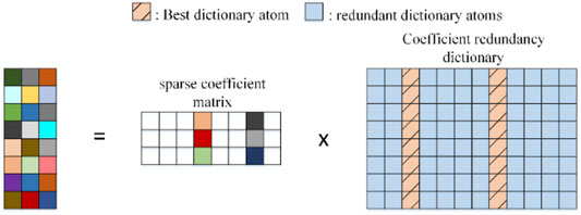
FIGURE 1. Sparse decomposition.

Then, hold the sparse representation matrix $T_i$ constant after the last iteration and optimize the base atom in the feature dictionary $D_{ti}$ separately. And the objective function can still be simplified. The update can be made as follows:

$J_{D_{ti}}=\arg \underset{D_{ti}}{\min }\left({\Vert G-{\displaystyle \sum _{j=1}^k{G}_i^j{T}_i^{j^L}}\Vert }_2^2\right)=\left({\Vert \left(G-{\displaystyle \sum _{j\ne k}{G}_i^j{T}_i^{j^L}}\right)-D_{ti}^k{T}_i^{k^L}\Vert }_2^2\right)=\left({\Vert G_k-G_i^k{T}_i^{k^L}\Vert }_2^2\right)(11)$

Where $k=\mathrm{1,2},\mathrm{...},N,$ $G_k$ are real error items, the SVD algorithm is used to decompose $G_k$, and the base atom $d_k$ that needs to be updated is the feature vector corresponding to the maximum eigenvalue, which can be computed by the least-square method. Then, the optimal feature dictionary $D_t$ is obtained, and the public dictionary $D_g$ is attained by the same method. The DCS learning dictionary $D$ is obtained by cascading $D_g$ and $D_t$ together. Therefore, the DCS learning dictionary can be expressed as follow:

$D=\left[\begin{array}{ccccc}{D}_g& D_t& 0& \cdots & 0\\ D_g& 0& D_t& \cdots & \\ \cdots & \cdots & \cdots & \cdots & 0\\ D_g& 0& \cdots & 0& D_t\end{array}\right](12)$

2.3 Data Storage Based on Cloud Edge Collaboration

Under the cloud-edge collaborative architecture (Ning et al., 2021), the DCS-OMP edge algorithm is used to compress and collect the power quality data of s nodes in a distribution system at the same time, the power quality data of each node in the distribution system share the same dictionary atoms, set the data length of each node as n and the number of uploaded dictionary atoms as τ, the corresponding formula is as follow:

$\left[{\mathit{Y}}_{m\times s}{\mathit{D}}_{\tau \times n}\right]=DC{S}_{-}SOMP\left({\mathit{X}}_{n\times s},{\mathbf{\Psi }}_{m\times n},{\mathbf{\text{Φ}}}_{n\times n},\tau ,SN{R}_{\text{d}\text{e}\text{f}? }\right)(13)$

$Y_{m\times s}$ is the measured value of each node; $X_{n\times s}$ is the original signal of each node, $D_{\tau \times n}$ is the uploaded dictionary atoms to the cloud. By reducing the length m of the measurement matrix and the number τ of the uploaded cloud dictionary atoms, the memory capacity of the measured values uploaded to the cloud, and the dictionary atoms can be reduced. In addition, in order to ensure that cloud data can be called accurately and quickly, the cloud integrates the dictionary atoms uploaded by each edge to generate a complete dictionary $D_{k\times n}$, where k is the total number of atoms in the complete dictionary. When calling data in this partition, the sparse representation coefficient corresponding to the partition data is calculated by the Eq. 13.

${\mathit{\theta }}_{n\times s}=SOMP\left({\mathit{Y}}_{m\times s},{\mathit{D}}_{k\times n},{\mathbf{\text{Ψ}}}_{m\times n}\right)(14)$

Then the original signal ${X^{\prime }}_{n\times s}$ of the partition is recovered through Eq. 13 as follow:

${{\mathit{X}}^{\prime }}_{n\times s}=real\left({\mathbf{\text{Φ}}}_{n\times n}{\mathit{\theta }}_{n\times s}\right)(15)$

By establishing a complete dictionary in the cloud center, each edge only needs to upload the measurement values to realize compression storage of power quality data, which reduces the storage space of cloud data. The steps for constructing a complete dictionary are as follows:

1) Calculate the correlation $r_{i,k}$ between the newly uploaded dictionary atom di of the edge node and the kth atom D_k in the initial sparse dictionary $D_{k\times n}$ in the cloud. The formula is as follow:

$r_{i,k}=\frac{\mathrm{cov}\left({\mathit{d}}_i,D_k\right)}{\sqrt{\mathrm{var}\left[{\mathit{d}}_i\right]\mathrm{var}\left[D_k\right]}}(16)$

Suppose the value of each generated is lower than a certain threshold. In that case, the overall correlation between the dictionary atom di uploaded to the cloud and the cloud dictionary $D_{k\times n}$ is relatively weak. Therefore, the dictionary atom is added to the sparse cloud dictionary.

2) Combine the dictionary atoms uploaded in each partition into an over-complete sparse dictionary, and regularization is performed to reduce the correlation between the dictionary atoms.

${\mathit{D}}_{k\times n}=\left\{{\mathit{d}}_1,{\mathit{d}}_2,\cdots ,{\mathit{d}}_k\right\}(17)$

${{\mathit{d}}^{\prime }}_{\mathit{k}}={\mathit{d}}_{\mathit{k}}-\frac{{\mathit{d}}_k,{{\mathit{d}}^{\prime }}_1}{{{\mathit{d}}^{\prime }}_1,{{\mathit{d}}^{\prime }}_1}{{\mathit{d}}^{\prime }}_1-\frac{{\mathit{d}}_{\mathit{k}},{{\mathit{d}}^{\prime }}_2}{{{\mathit{d}}^{\prime }}_2,{{\mathit{d}}^{\prime }}_2}{{\mathit{d}}^{\prime }}_2-\cdots -\frac{{\mathit{d}}_{\mathit{k}},{{\mathit{d}}^{\prime }}_{\mathit{k}-1}}{{{\mathit{d}}^{\prime }}_{\mathit{k}-1},{{\mathit{d}}^{\prime }}_{\mathit{k}-1}}{{\mathit{d}}^{\prime }}_{\mathit{k}-1}(18)$

3) Normalizes the over-complete dictionaries to update dictionary atoms.

${\mathit{d}}_{\mathit{k}}=\frac{{{\mathit{d}}^{\prime }}_{\mathit{k}}}{{{\mathit{d}}^{\prime }}_{\mathit{k}}}(19)$

4) Combined with the over-complete sparse dictionary, recover the original data from the measured values uploaded by the DCS algorithm to verify the recoverability of the stored data and the corresponding sparse coefficient θ_j, j∈[1,s] of each node is obtained. Finally, the compressed storage of power quality data of each node is realized.

Cloud computing is a type of technology that enables the analysis of large amounts of data (Luo, 2022). It is not required to maintain computing hardware, data storage, or associated software on-premises. However, because of the physical separation between the cloud platform and each terminal, response times are frequently slow.

Edge computing is introduced as a novel technique for augmenting cloud computing systems (Ma et al., 2021). Because the edge is located close to the terminal equipment, it can reduce not only the network delay associated with data processing, but also the bandwidth required to transfer the original data to the storage center. As a result of the cloud platform and edge platform collaborating, the system’s performance will be significantly improved.

In this paper, based on the cloud-edge collaboration framework shown in Figure 2, the edge acquisition algorithm based on DCS-SOMP algorithm is compiled on the MATLAB simulation platform to collect the power quality data generated in PSCAD, and the sparse dictionary atoms and measured values generated in the reconstruction process are uploaded to the cloud server by establishing a connection with the remote cloud. There are three main operations in the cloud: 1) compressed storage of power quality data of distribution network; 2) Construction of complete sparse dictionary; 3) Analysis and calculation of power quality data. The cloud server sends the result of dynamic partition to the edge in time. The edge algorithm obtains the new partition information, adjusts the computing resources, and collects the power quality contained in the new partition, and uploads it to the cloud server again. So as to realize the mutual cooperation between “cloud” and “edge”.

FIGURE 2

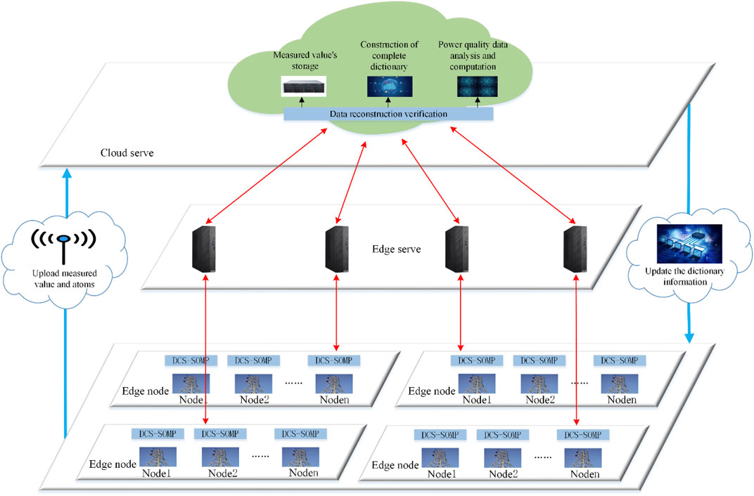
FIGURE 2. Cloud-edge collaboration framework.

3 Power Quality Data Classification

3.1 Classification of Power Quality Disturbance Signals

The PQD classification model first extracts the characteristics of the disturbance signals and then designs a classifier to recognize different disturbances. According to the different characteristics of amplitude, frequency, and phase of the disturbance signal, the single disturbance is defined as voltage sag, voltage swell, short interruption, harmonic, transient oscillation, pulse, and flicker. The three disturbances of voltage sag, voltage swell, and short interruption are short-term root mean square fluctuations. And the harmonic, transient oscillation, pulse, and flicker are long-term root mean square fluctuation or high-frequency impact disturbance. In addition to the above single disturbance, disturbance usually occurs simultaneously in the actual situation, which is called composite disturbance. The composite disturbance is compounded by two or more single disturbances, which is difficult to analyze. Referring to the IEEE standard and previous literature, six types of single disturbances and four types of composite disturbances are analyzed in this paper.

3.2 Basic Principle of Power Disturbance Classification Based on CS-DL

3.2.1 The Framework of CS-DL Network

A Deep Neural Network (DNN) is the basis of deep learning, which is a multi-layer expression algorithm for learning the implicit distribution of data. Specifically, DNN first employs unsupervised learning to pre-train each layer to learn the characteristics of layers. Training one layer at a time, using the results as the input to the next layer, and then using supervised learning to fine-tune the model from top to bottom. The feature learning process is illustrated in Figure 3.

FIGURE 3

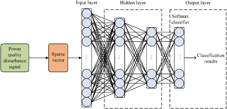
FIGURE 3. Structure of CS-DL network.

The feature of the constructed CNN is the feature extractor composed of the convolution layer and the sub-sampling layer. The CS-DL network uses a local connection, which only connects one neuron with a few peripheral neurons. The convolution layer of CNN contains multiple differentiated feature planes, each of which consists of some rectangularly arranged neurons, and the neurons on the same feature plane share weight with each other. CNN sub-sampling is a special convolution process and reduces the number of model parameters. In summary, CNN uses the convolution layer and sub-sampling layer, as well as the corresponding local connection and weight sharing rules to enhance feature extraction’s self-learning and characterization capacity and finally realizes the classification of direct power quality signal inputs.

3.2.2 Structures of CNN-BiLSTM and CS-BiLSTM Networks

PQD signal is a typical time-series signal, but CNN does not consider the timing characteristics of the signals in the process of feature extraction. Meanwhile, the bidirectional long short-term memory (BiLSTM) model is a kind of Recurrent Neural Network (RNN) suitable for time-series signal analysis. Therefore, a mixed CNN-BiLSTM model based on the classification of PQD signals by the CNN model is proposed. Firstly, features of disturbing signals are extracted automatically by CNN. Then, the features are further processed by BiLSTM. The proposed CNN-BiLSTM model enhances the feature extraction ability of the model, speeds up the convergence rate of training, further improves the accuracy of disturbance classification, and has high noise immunity. In order to deal with the time-consuming defect and classification problem of composite disturbance, an improved CS-BiLSTM is proposed, which utilizes the CS method to transmit signal characteristics quickly, accurately, and effectively so as to improve the efficiency and timeliness of the PQD classification process.

The Structures of CS-BiLSTM Networks are illustrated in Figure 4.

FIGURE 4

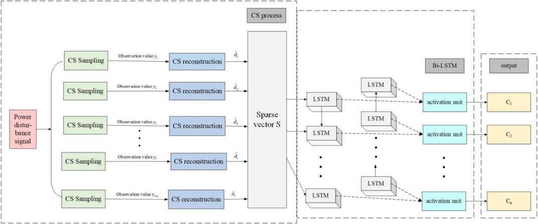
FIGURE 4. Structure of CS-BiLSTM.

3.3 Parameter Optimization Based on DDPG

3.3.1 Concept of Reinforcement Learning

Reinforcement learning achieves global optimization of the objective function through the feedback of the reward function. The main parts of the DDPG reinforcement learning algorithm are as follows:

Agent: The agent that needs to be controlled, corresponding to the parameter optimizer in this paper.

State s: The agent’s current state, corresponding to the current value of the key parameters such as learning rate, minibatch number, etc.

Action a: The actions that the agent can take, corresponding to the variation of the parameters.

Reward r: The feedback value of the environment, and the evaluation value of the previous action, corresponding to the accuracy in this paper.

$\pi$ The agent’s action to move from the current state to the next state.

Value: The reward value of the agent’s long-term actions, as distinguished from the short-term reward represented by Reward r.

Environment: The environment in which the agent is placed.

3.3.2 Concept of Deterministic Policy Gradient

Deterministic Policy Gradient (DPG) is an improved algorithm based on AC (Action and Critic) structure. It utilizes the PG (Policy Gradient)’s advantage in continuous space and changes the randomized strategy to a deterministic strategy. The corresponding formula is shown in (20):

$a_t\sim {\pi }_{\theta }\left(s_t|{\theta }^{\pi }\right)(20)$

The DPG method can reduce the sampling size of data. For randomized strategy, policy gradient needs to integrate state and action simultaneously, and determine strategy only needs to integrate the state, which greatly improves the algorithm’s efficiency. The formulas of deterministic strategy and the gradient expression are as follows:

$J_{\beta }\left(\mu \right)=E_{S\sim {\rho }^{\beta }}\left[Q^{\mu }\left(s,\mu \left(s\right)\right)\right](21)$

${\mathrm{\nabla }}_{\theta }J\left({\mu }_{\theta }\right)=E_{S\sim {\rho }^{\beta }}\left[{\mathrm{\nabla }\theta {\mu }_{\theta }\left(s\right)Q^{\mu }\left(s,a\right)|}_{a={\mu }_{\theta }}\right](22)$

Where: $\mu$ represents the determined strategy adopted by DDPG, ${\rho }^{\beta }$ represents the distribution of a balanced exploration and utilization process. In the DPG algorithm, the Critic network is a linear function approximator, and the Actor updates the parameters in the direction of the Critic’s action-value function.

The DDPG algorithm is improved by the following details: the updating methods of the target network’s parameters, the regularization method of the samples, and the exploration noise of action. Compared with DQN (Deep Q network), which updates the parameters of the target network at regular time intervals, DDPG adopts a soft update method, which transfers the parameters both before and after updating to the target network. In order to prevent gradient disappearance or exploding gradient, the input and output of ANN are normalized in batches. Moreover, the DDPG algorithm adds a Gaussian noise to the determined action to improve the diversity of samples.

3.4 CS-BILSTM Model Based on DDPG Optimization

The complexity of PQD classification is prone to result in no convergence and poor training effects for the classification model. Therefore, the DDPG method is introduced to optimize the parameters during the training process. The DDPG algorithm based on artificial intelligence has the characteristics of self-organization, self-adaptation, and self-learning, has high robustness, and is easy to parallel. The detailed parameter of the DDPG network is set as follows. The inputs of the Actor network are normally N × 2 sequences with two hidden layers which has 256 and 32 neurons respectively. The activation function of the Actor network is tanh, the loss function is MSE, and the optimization method RMSprop is introduced here. The input of Critic network consists of two parts: the first part is the state observed by the agent; The second part is the corresponding actions taken by the agent. The hidden layer includes two layers, the number of neurons is 256 and 32 respectively, and the number of neurons in the output layer is 1, which indicates the Q value obtained by the critical network taking some action in this state. Except for the output layer, other activation functions use tanh, and the activation function of the output layer is Relu. After obtaining the Q value, the probability of generating random action is ε Strategy, i.e., probability 1- ε chooses ${\pi }^{\ast }\left(s\right)=\arg \max Q\left(s,a\right)$. Meanwhile, the value of random action follows the normal distribution , $\sigma ={\left(Q\left(s,a\right)-\arg \max \left(Q\left(s,a\right)\right)\right)}^2$. The related Param-eter setting and description of DDPG algorithm is shown in APPENDIX part.

It is widely used in the optimization of multimodal functions. The traditional stacked denoising autoencoder adopts SGD in the fine-tuning stage. The SGD updates each sample with a fast update rate, which can automatically pick out the inferior local optimtbal points. However, on account of the many update times, the cost function may experience acute fluctuation with inferior convergence performance, which affects the classification effect of the encoder. Therefore, this paper improves the traditional DAE. Adam is used to updating the network weights and bias during the fine-tuning stage instead of SGD. The flow chart of PQD classification by the improved CS-BiLSTM algorithm based on DDPG parameter optimization is illustrated in Figure 5.

FIGURE 5

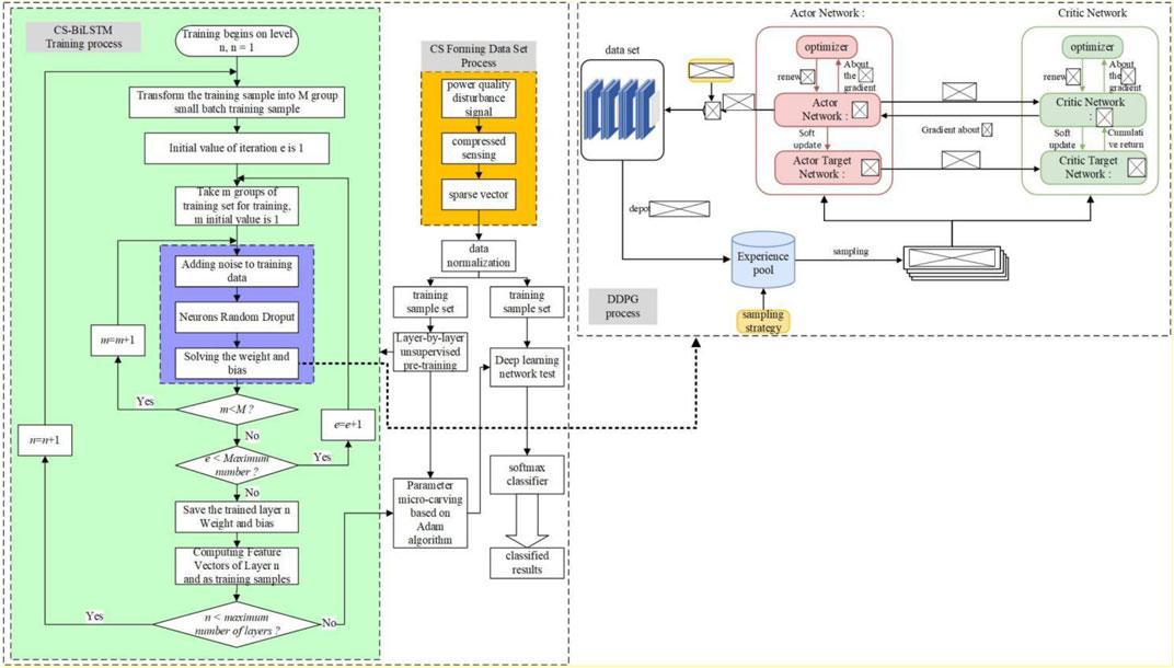
FIGURE 5. Schematic diagram of the CS-BILSTM model optimized by DDPG algorithm.

4 Simulation Results and Analysis

The proposed power quality signal compression technique and PQD classification are evaluated in this section via the comparative experiments with four simulation tests. The simulation software are respectively Matlab2019b and Python3.6.5 with its advanced tool pytorch1.2.0. As for the computer configuration, the Intel Core CPU i3-8100 and internal storage 16G with the 1T hard disk storage device.

This paper uses the WAMS (Wide Area Measurement System) data collected from the actual power grid in a province of China in 2020 to form a data set. The data set is the power quality data that has been manually verified, including 2000 pieces of data. In order to form the enough training set, some power quality data is generated with the MATLAB simulation.

A series of power quality signals are generated by mathematical modeling simulation, and the sampling frequency is set to 3200 Hz based on the actual sampling frequency of power equipment in the power system. Also, the power quality signal sampling length is 18 cycles.

Then, the Gaussian white noise is added in the generation of the PQD signal to simulate the random noise in the power system. The signal-to-noise ratio (SNR) ranges from 20 dB to 40 dB.

The generated power quality signals include six categories of single disturbance and four types of composite disturbance such as voltage sag, harmonic, voltage flicker, harmonic with voltage sag, harmonic with voltage interruption, voltage sag with voltage flicker, etc. They are all labeled with the number from 1 to 10, respectively.

MATLAB is used to generate 20,000 sets of PQD signals, where 18,000 sets are chosen as the training set, and the last 2000 sets are selected as the testing set. The 10-fold cross-validation is adopted to select the suitable training set and validation set in this step. Figure 7 demonstrates the experiment result.

4.1 Comparison Results of Reconstruction Algorithms

As shown in Figure 6, Orthogonal Matching Pursuit, Generalized Orthogonal Matching Pursuit (Generalized OMP, GOMP), Regularized Matching Pursuit (Regularized OMP, ROMP), and Stage Orthogonal Matching Pursuit (StagewiseOMP, StOMP), Compressive Sampling Matching Pursuit (CompressiveSamplingMP, CoSaMP), and DCS-SOMP algorithms are adopted to perform compressive sampling of PQD signals in the power grid, while the sparsity of the PQD signal of each node is assumed as 10. The comparison of the signal-to-noise ratios (SNR) of reconstructed power quality signals under different compression ratios is carried out between the above algorithms. Figure 5 demonstrates that except for the DCS-SOMP algorithm, the signal-to-noise ratio of other algorithms’ reconstructed power quality signals decreases with the increase of compression ratio. In the subfigure (a) of Figure 5, the reconstructed power quality signals of the ROMP and CoSaMP algorithms show distortion when the compression ratio rises to 40. Additionally, in the process of power quality data compression and storage, the sparsity of PQD signals under the sparse dictionary has an important impact on the power quality data’s upload speed to the cloud. The sparser the data, the fewer sparse dictionary atoms, thus, the smaller data sizes. By contrast, the DCS-SOMP reconstruction algorithm overperform other algorithms, like OMP, ROMP, etc. It is clearly more accurate for the compressed acquisition of power quality data.

FIGURE 6

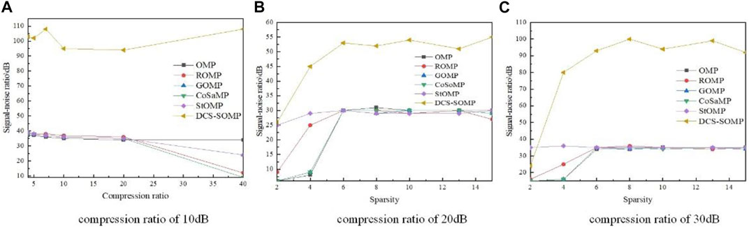
FIGURE 6. Comparison of reconstruction effects. (A) Compression ratio of 10 dB, (B) Compression ratio of 20 dB, and (C) Compression ratio of 30 dB.

4.2 Reconstruction and Demonstration of Different Power Quality Disturbances

After determining the transform domain, the measurement matrix, and the reconstruction algorithm, the compression-reconstruction simulation of 6 types of PQD signals is carried out, and the compression rate represents the ratio of the observation points’ number to the signal length, which is set as 25%. In order to reduce the reconstruction error, the sparsity value of different disturbance signals in Table 1 is determined through a large number of experiments. Moreover, Table 1 shows the error values between the original signal and the reconstructed PQD signal obtained by compressed sensing and reconstructing of randomly generated PQD signals. Figure 7 shows the simulation diagrams of the original signals, the reconstruction signals, and the error waveform of the two kinds of PQD signals. Finally, we use mean square error to evaluate the reconstruction signals.

TABLE 1

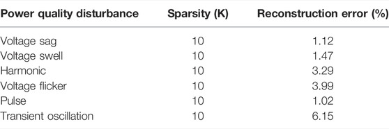
TABLE 1. Reconstruction error of power quality disturbance signal.

FIGURE 7

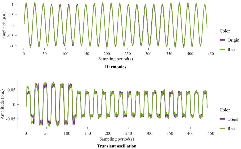
FIGURE 7. Simulation waveform of the original signal and reconstructed signal.

4.3 Comparison of Application of CS-DL in Power Quality Disturbance Classification

4.3.1 Results of Power Quality Disturbance Classification

It can be seen from Figure 8 that the classification accuracy of PQD signals is still relatively low in the initial stage of training. Then, the loss value is quickly reduced to less than 0.1 after about 850 epochs of training. Also, the classification accuracy is improved to about 94% and remains stable, which indicates that the network converges after about 850 training epochs. Moreover, the training accuracy and test accuracy are almost equal after about 950 epochs of training, and the total classification accuracy of PQD signals in the test set is 99.7%. In order to obtain better network performance, the setting of the network parameters is necessary, in which the setting of the learning rate is critical. In this paper, the dynamic setting method of learning rate is adopted. The initial learning rate is set to 0.001; after 200 iterations, it drops to 0.0001. This setting can further improve the classification accuracy of PQD signals.

FIGURE 8

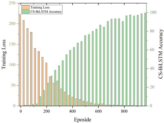
FIGURE 8. Training loss and classification accuracy of CS-BiLSTM model.

It can be seen from Figure 9, Figure 10, and Table 2 that the CS-BiLSTM method we proposed has a superior performance compared with the CNN-BiLSTM method in the classification of PQD. Although the CS-BiLSTM model has lower classification accuracy for voltage flicker and transient oscillation than the CNN-BiLSTM model, the CS-BiLSTM has higher classification accuracy in the other eight types of PQD and average classification accuracy. Meanwhile, the CS-BiLSTM model’s training time is only 59.12% of the CNN-BiLSTM model’s training time. Since the voltage sags, voltage swells, and harmonics account for more than 70% of the PQD types, in reality, the ten types of PQD samples are also created in proportion.

FIGURE 9

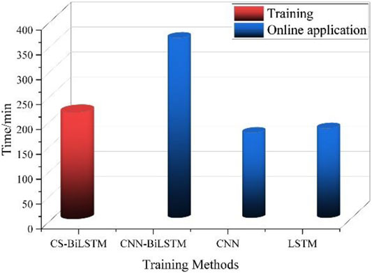
FIGURE 9. Comparison of training time.

FIGURE 10

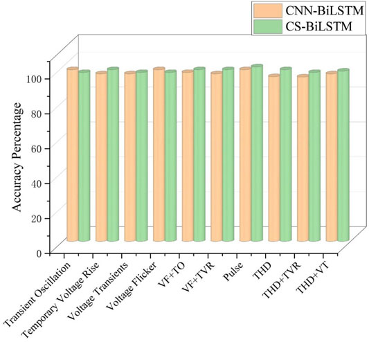
FIGURE 10. Classification results of non-noise power quality disturbance signals.

TABLE 2

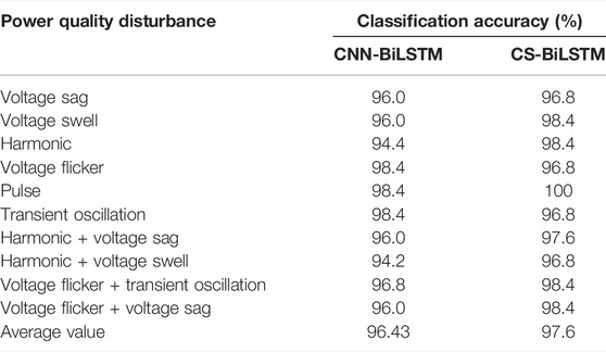
TABLE 2. Classification accuracy of the reconstructed signal.

In the case of identifying 1,000 groups of voltage sag disturbance data, 730 groups are classified as voltage sags, 80 groups are identified as oscillation with voltage sags, 20 groups are identified as voltage flicker with voltage sags, and 180 groups are identified as harmonic with voltage sags. Furthermore, we analyze the 180 groups of signals that are identified as composite disturbances of harmonic with voltage sags. The analysis shows that there exist harmonic components in these signals, which meet the requirements of IEEE standard for harmonic definition. In addition, it indicates that the label of some original data is inaccurate. Meanwhile, the result demonstrates that the proposed method has high classification accuracy for composite disturbances, which is normally neglected in the previous study. The total classification time of the CS-BiLSTM model for the 1,000 groups of voltage sags data is 15 s, with an average classification time of 0.15 s per sample.

4.3.2 Results of Parameter Optimization Based on DDPG Method

Three Gaussian white noises were added to the initial signal to verify the noise immunity of the algorithm before training, and the SNR is 20 dB, 30 dB, and 40 dB, respectively, after adding the Gaussian noise. As shown in Figure 11, the accuracy rate of PQD classification increases rapidly in the initial stage of training. After about 400 rounds of training and learning, the loss value decreases rapidly to less than 0.2. The classification accuracy rate increases to about 95% and then remains stable, indicating that the network has converged. Compared with the traditional method, the proposed method has a superior performance of PQD classification both under simple situations and in the case of complex PQD.

FIGURE 11

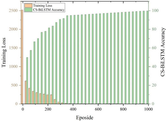
FIGURE 11. Training loss and classification accuracy of the optimized CS-BiLSTM model.

It can be seen from Figure 12 and Table 3 that with the increase of noise, the average classification accuracy of the two methods for PQD is gradually reduced. When the noise intensity is 40 and 30 dB, the average classification accuracy of the CS-BiLSTM model is 97.49 and 96.76%, respectively. When the noise intensity is further strengthened to 20 dB, the classification accuracy is significantly reduced to 96.07% but remains high. Compared with the CNN-BiLSTM model, the CS-BiLSTM hybrid model performs a higher classification accuracy obviously for all types of PQDs. The experimental results fully prove that the proposed hybrid model possesses a good classification ability of PQD signals and has promising anti-noise capability.

FIGURE 12

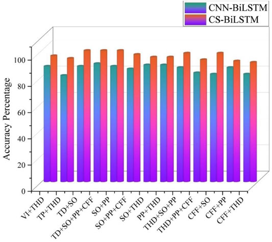
FIGURE 12. Classification results of power quality disturbance signals with 20 dB compression ratio.

TABLE 3

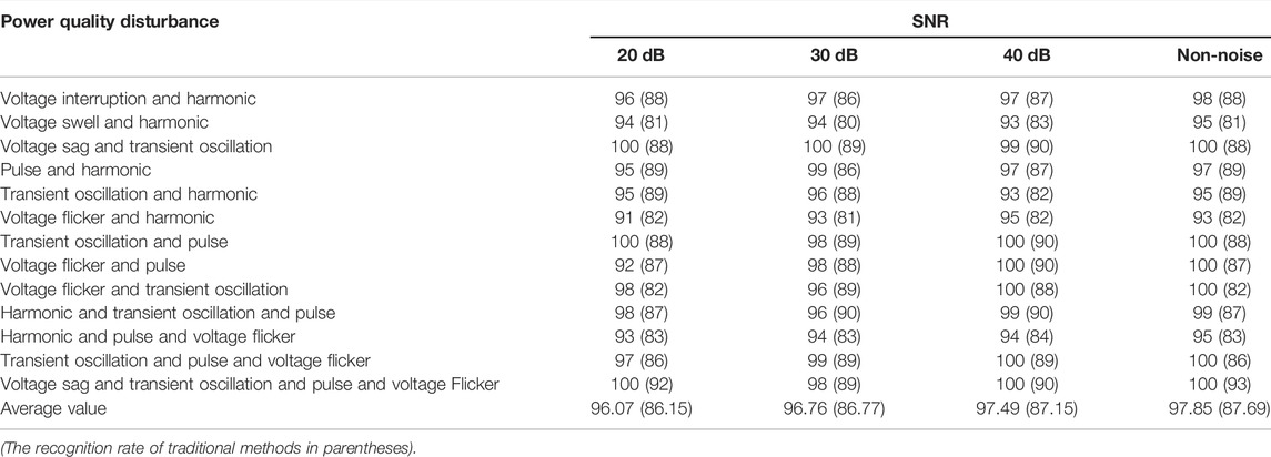
TABLE 3. Classification results of multiple disturbances.

5 Conclusion

This paper presents a power quality disturbance classification and classification method based on DCS and deep learning. Through this method, the efficient compression and accurate reconstruction of power quality data of each node in the power grid can be realized. Moreover, the identification and classification of PQDs in the power grid can be realized, which provides a new reference for the governance of power grid harmonics and the storage of power quality data. The main conclusions of this paper are as follows:

1) Based on the SOMP algorithm and K-SVD dictionary learning algorithm, a DCS algorithm called DCS-OMP is proposed, which realizes efficient compression and accurate reconstruction of power quality data in distribution network under low measurement value and high compression ratio.

2) Based on the CNN-BiLSTM model, a CS-BiLSTM hybrid model is built, and a comparison is carried out between the two models. The average recognition rate of CS-BiLSTM hybrid model is 97.85% without noise, and 97.49, 96.76, and 96.07% with 40, 30, and 20 dB noise, respectively. Compared with the CNN-BiLSTM model, the recognition rate of the CS-BiLSTM hybrid model is increased by 10.15, 10.30, 10.00, and 9.23% in the case of no noise, 40 dB noise, 30 dB noise, and 20 dB noise, respectively. The recognition rate in high-intensity noise interference is improved significantly. According to the results, the proposed CS-BiLSTM hybrid model has a higher recognition rate and better noise immunity.

3) DDPG algorithm is employed to optimize the parameters in the training process of the CS-BiLSTM hybrid model, which ensures the convergence of training and the effectiveness of results.

The proposed method CS-BiLSTM is more efficient to solve the problems of high sampling rate, high cost of hardware implementation when performing the disturbance recognition of power quality data. It helps improve the related theory and algorithm of power quality analysis and detection. However, the application of parameters optimization via reinforcement learning will inevitably encounter spending much time training the network. In the future, we would like to further adjust the parameters to make the experiment converge, speed up the convergence speed of the network, reduce the time spent on training and improving the computing efficiency of the algorithm.

Data Availability Statement

The original contributions presented in the study are included in the article/Supplementary Material, further inquiries can be directed to the corresponding author.

Author Contributions

XX: Drafting the manuscript, CH: experimental analysis, HC: Review and Supervision, YL: Methodology and Formal analysis, BZ: Conceptualization and Revised, SW: Data Curation and Resources, CC: Software.

Funding

This work is supported by The Laboratory Open Fund of Beijing Smart-chip Microelectronics Technology Co., Ltd.

Conflict of Interest

Authors XX and CH were employed by Beijing Smart-Chip Microelectronics Technology Co., Ltd Authors YL, BZ, and SW were employed by Beijing Electric Power Science and Smart Chip Technology Company Limited.

The authors declare that this study received funding from The Laboratory Open Fund of Beijing Smart-chip Microelectronics Technology Co., Ltd. The funder had the following involvement in the study: data collection, experiment analysis.

Publisher’s Note

All claims expressed in this article are solely those of the authors and do not necessarily represent those of their affiliated organizations, or those of the publisher, the editors and the reviewers. Any product that may be evaluated in this article, or claim that may be made by its manufacturer, is not guaranteed or endorsed by the publisher.

References

Berutu, S. S., and Chen, Y. C. (2020). “Power Quality Disturbances Classification Based on Wavelet Compression and Deep Convolutional Neural Network,” in 2020 International Symposium on Computer, Consumer and Control (IS3C).IEEE, Taichung City, Taiwan, 13-16 Nov. 2020, 327–330.

CrossRef Full Text | Google Scholar

Bravo-Rodríguez, J. C., Torres, F. J., and Borrás, M. D. (2020). Hybrid Machine Learning Models for Classifying Power Quality Disturbances: A Comparative Study. Energies 11 (13), 2761–2768. doi:10.3390/en13112761

CrossRef Full Text | Google Scholar

Cai, K., Cao, W., Aarniovuori, L., Pang, H., Lin, Y., and Li, G. (2019). Classification of Power Quality Disturbances Using Wigner-Ville Distribution and Deep Convolutional Neural Networks. IEEE Access 7 (1), 119099–119109. doi:10.1109/ACCESS.2019.2937193

CrossRef Full Text | Google Scholar

Chen, S. (2003). A Quantitative Analysis of the Data Acquisition Requirements for Measuring Power Quality Phenomena. IEEE Trans. Power Deliv. 18 (4), 1575–1577. doi:10.1109/TPWRD.2003.817521

CrossRef Full Text | Google Scholar

Elphick, S., Ciufo, P., Drury, G., Smith, V., Perera, S., and Gosbell, V. (2017). Large Scale Proactive Power-Quality Monitoring: An Example from Australia. IEEE Trans. Power Deliv. 32 (2), 881–889. doi:10.1109/TPWRD.2016.2562680

CrossRef Full Text | Google Scholar

Elphick, S., Gosbell, V., Smith, V., Perera, S., Ciufo, P., and Drury, G. (2017). Methods for Harmonic Analysis and Reporting in Future Grid Applications. IEEE Trans. Power Deliv. 32 (2), 989–995. doi:10.1109/TPWRD.2016.2586963

CrossRef Full Text | Google Scholar

Gibbon, T. B., Yu, X., and Monroy, I. T. (2009). Photonic Ultra-wideband 781.25-Mb/s Signal Generation and Transmission Incorporating Digital Signal Processing Detection. IEEE Photon. Technol. Lett. 21 (15), 1060–1062. doi:10.1109/LPT.2009.2022503

CrossRef Full Text | Google Scholar

Jin, L., Haosong, L., Zhongping, X., Ting, W., Shuai, W., Yutong, W., et al. (2019). “Research on Wide-Area Distributed Power Quality Data Fusion Technology of Power Grid,” in 2019 IEEE 4th International Conference on Cloud Computing and Big Data Analysis (ICCCBDA), Chengdu, China, 12-15 April 2019, 185–188. doi:10.1109/icccbda.2019.8725668

CrossRef Full Text | Google Scholar

Li, L., Liu, P., Wu, J., Wang, L., and He, G. (2020). Spatiotemporal Remote-Sensing Image Fusion with Patch-Group Compressed Sensing. IEEE Access 8, 209199–209211. doi:10.1109/ACCESS.2020.3011258

CrossRef Full Text | Google Scholar

Li, Y., Zhang, M., and Chen, C. (2022). A Deep-Learning Intelligent System Incorporating Data Augmentation for Short-Term Voltage Stability Assessment of Power Systems. Appl. Energ. 308, 118347. doi:10.1016/j.apenergy.2021.118347

CrossRef Full Text | Google Scholar

Lu, W., Wei, Y., Yuan, J., Deng, Y., and Song, A. (2020). Tractor Assistant Driving Control Method Based on EEG Combined with RNN-TL Deep Learning Algorithm. IEEE Access 8, 163269–163279. doi:10.1109/ACCESS.2020.3021051

CrossRef Full Text | Google Scholar

Luo, F. (2022). Data-Driven Energy Demand Side Management Techniques. Front. Energ. Res., 24. doi:10.3389/fenrg.2022.849031

CrossRef Full Text | Google Scholar

Ma, F., Wang, B., Li, M., Dong, X., Mao, Y., Zhou, Y., et al. (2021). Edge Intelligent Perception Method for Power Grid Icing Condition Based on Multi-Scale Feature Fusion Target Detection and Model Quantization. Front. Energ. Res. 9, 591. doi:10.3389/fenrg.2021.754335

CrossRef Full Text | Google Scholar

Negnevitsky, M., Faybisovich, V., Santoso, S., Powers, E. J., Grady, W. M., and Parsons, A. C. (2000). Discussion of "Power Quality Disturbance Waveform Recognition Using Wavelet-Based Neural Classifier-Part 1: Theoretical Foundation. IEEE Trans. Power Deliv. 15 (4), 1347–1348. doi:10.1109/61.891571

CrossRef Full Text | Google Scholar

Ning, L., Si, L., Nian, L., and Fei, Z. (2021). Network Reconfiguration Based on Edge-Cloud-Coordinate Framework and Load Forecasting. Front. Energ. Res. 9, 525. doi:10.3389/fenrg.2021.679275

CrossRef Full Text | Google Scholar

Noland, K. C. (2016). High Frame Rate Television: Sampling Theory, the Human Visual System, and Why the Nyquist–Shannon Theorem Does Not Apply. SMPTE Motion Imaging J. 125 (3), 46–52. doi:10.5594/JMI.2016.2531998

CrossRef Full Text | Google Scholar

Pei, S., Hsue, W., and Ding, J. (2006). Discrete Fractional Fourier Transform Based on New Nearly Tridiagonal Commuting Matrices. IEEE Trans. Signal Process. 54 (10), 3815–3828. doi:10.1109/TSP.2006.879313

CrossRef Full Text | Google Scholar

Song, Z., Liu, B., Pang, Y., Hou, C., and Li, X. (2012). An Improved Nyquist–Shannon Irregular Sampling Theorem from Local Averages. IEEE Trans. Inf. Theor. 58 (9), 6093–6100. doi:10.1109/TIT.2012.2199959

CrossRef Full Text | Google Scholar

Tang, Q., Qiu, W., and Zhou, Y. (2020). Classification of Complex Power Quality Disturbances Using Optimized S-Transform and Kernel SVM. IEEE Trans. Ind. Electro. 67 (61), 9715–9723. doi:10.1109/TIE.2019.2952823

CrossRef Full Text | Google Scholar

Uçkun, F. A., Özer, H., Nurbaş, E., and Onat, E. (2020). “Direction Finding Using Convolutional Neural Networks and Convolutional Recurrent Neural Networks,” in 2020 28th Signal Processing and Communications Applications Conference (SIU), Gaziantep, Turkey, 5-7 Oct. 2020, 1–4. doi:10.1109/SIU49456.2020.9302448

CrossRef Full Text | Google Scholar

von Gladiß, A., Ahlborg, M., Knopp, T., and Buzug, T. M. (2015). Compressed Sensing of the System Matrix and Sparse Reconstruction of the Particle Concentration in Magnetic Particle Imaging. IEEE Trans. Magnetics 51 (2), 1–4. doi:10.1109/TMAG.2014.2326432

CrossRef Full Text | Google Scholar

Xin, R., Zhang, J., and Shao, Y. (2020). Complex Network Classification with Convolutional Neural Network. Tsinghua Sci. Technol. 25 (4), 447–457. doi:10.26599/TST.2019.9010055

CrossRef Full Text | Google Scholar

Yin, M., Xu, Y., Shen, C., Liu, J., Dong, Z. Y., and Zou, Y. (2017). Turbine Stability-Constrained Available Wind Power of Variable Speed Wind Turbines for Active Power Control. IEEE Trans. Power Syst. 32 (3), 2487–2488. doi:10.1109/TPWRS.2016.2605012

CrossRef Full Text | Google Scholar

Zhang, M., Li, J., Li, Y., and Xu, R. (2021). Deep Learning for Short-Term Voltage Stability Assessment of Power Systems. IEEE Access 9, 29711–29718. doi:10.1109/access.2021.3057659

CrossRef Full Text | Google Scholar

Zhao, W., Shang, L., and Sun, J. (2019). Power Quality Disturbance Classification Based on Time-Frequency Domain Multi-Feature and Decision Tree. Prot. Control. Mod. Power Syst. 4 (1), 1–6. doi:10.1186/s41601-019-0139-z

CrossRef Full Text | Google Scholar

Appendix

TABLE A1

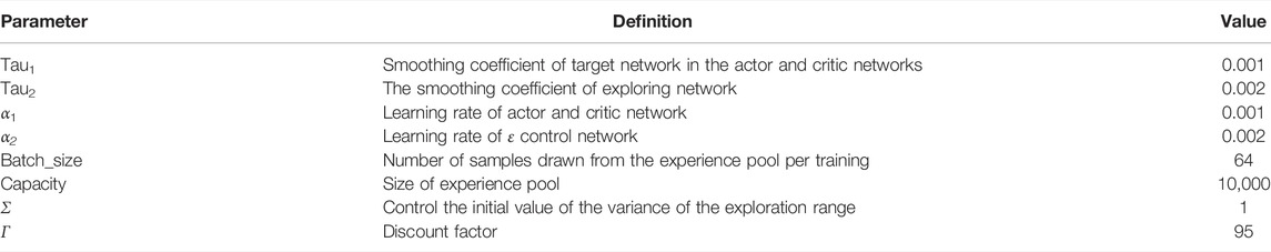
TABLE A1. Parameter setting and description of DDPG algorithm.