Investigation of Nodal Numerical Adjoints From CMFD-Based Acceleration Methods

In this work, the attribute of mathematical adjoints acquired from various CMFD (coarse-mesh finite difference) accelerated nodal methods based on the nodal expansion method (NEM) is presented. The direct transposition is implemented to the NEM-CMFD system matrix that includes correction factors to acquire the adjoint flux. Three different acceleration schemes are considered in this paper, which are, namely, CMFD, pCMFD, and one-node CMFD methods, and the self-adjoint attribute of migration operator for each acceleration scheme is studied. With regard to the one-node CMFD acceleration, a mathematical description for encountering negative adjoint flux values is given alongside an adjusted one-node CMFD scheme that stifles such an occurrence. The overall features of the aforementioned acceleration methods are recognized through analyses of 2D reactor problems including the KWU PWR 2D benchmark problem. Further systematic assessment is conducted based on the first-order perturbation theory, where the obtained adjoint fluxes are applied as weighting functions. It is clearly shown that the adjusted one-node CMFD scheme results in an improved reactivity estimation by excluding the presence of negative adjoint flux values.

Introduction

The adjoint flux is often referred to as an importance function since it signifies the importance of a neutron source at a certain phase-space contributing to fission reaction. Mathematically, it could be shown that the first-order errors can be removed when the adjoint flux is utilized as a weighting function, rendering it to be a preferred choice for perturbation theory–based analyses and generation of point kinetic parameters (Ott and Neuhold, 1985). The appraisal of adjoint flux can be performed by solving either the balance equation for itself or the transpose of a balance equation for the forward flux. The acquired adjoint fluxes from the former and latter methods are usually referred to as physical and mathematical adjoint fluxes, respectively.

Notwithstanding the presented advantages of an adjoint flux, its acquisition related to nodal methods is often regarded to be obscure. It is worthwhile to articulate that the reactor balance equation of interest is a well-defined problem, which implies the accuracy of nodal solution can be retained when corresponding current information is preserved. From such a perspective, correction factors for the finite difference method (FDM) can be envisioned, which forces the net current acquired from FDM-like representation to concur with that of the standalone nodal solution. Whereupon, acceleration in the nodal calculation can be met, which is known as the coarse-mesh finite difference (CMFD) method (Smith, 1983).

The meaning of the physical adjoint flux, which is obtained through discretization of balance equation for the adjoint flux itself, is still subjected to ambiguity issues (Lewins, 1965). The inclusion of discontinuity factors or super homogenization factors, i.e., nodal equivalence theory, additionally complicates the proper interpretation of physical adjoint.

On the contrary, the mathematical adjoint, which can be harnessed via solving the transposed balance equation for the forward flux, can be envisaged (Lawrence, 1984). However, the direct transposition of continuous balance equation is not practical and rather ambiguous for nodal methods that rely on the usage of transverse leakage (Hong and Cho, 1995). A different measure can be taken by transposing the discretized balance equation under CMFD accelerated nodal methods, where transverse leakage and its associated complexities are incorporated via the correction factors in the system matrix. The former and the latter ones are often referred to as direct-mathematical adjoint and indirect-mathematical adjoint, respectively. It is the latter approach that is widely implemented, which will be cited as numerical adjoint throughout this work.

A previous work states that negative adjoint flux values could occur for the conventional CMFD method, which utilized the analytic nodal method (ANM) solution while deducing the correction factor (Müller, 2014). To overcome such an unphysical anomaly, an additional correction was proposed; however, it deteriorates the consistency of CMFD formulation. In addition, no systematic evaluation of numerical adjoints from different CMFD schemes has been conducted.

In this paper, the characteristics of numerical adjoint fluxes obtained from nodal expansion method (NEM) solutions accelerated via various CMFD schemes are investigated. Especially, a systematic comparison is conducted between each adjoint flux obtained from different CMFD schemes, e.g., conventional CMFD, partial current–based CMFD, and one-node CMFD, based on the first-order perturbation theory. In Coarse-Mesh Finite Difference–Based Acceleration Methods, the basic concept and mathematical formulas regarding various CMFD acceleration schemes are depicted. In Nodal Expansion Method, a brief explanation concerning the nodal expansion method is given. In Attributes of Numerical Adjoint Flux, mathematical descriptions for attributes of numerical adjoints are depicted including the occurrence of negative adjoint flux. In Numerical Results, numerical results are presented alongside first-order perturbation theory–based comparison. Finally, conclusions are given in Conclusion.

Coarse-Mesh Finite Difference–Based Acceleration Methods

The philosophy of the CMFD acceleration scheme is the preservation of the reference net current information while retaining the formulation of the finite difference method (FDM), which is the simplest numerical measure to be taken. Three different CMFD-based acceleration methods are considered in this work, which are, namely, 1) conventional CMFD, 2) partial current–based CMFD (pCMFD), and 3) one-node CMFD.

Conventional CMFD Method

Figure 1 illustrates the balance for neutron flux within a node of interest i, and its associated balance equation is expressed as follows:

${\overline{J}}_{i,i+1}-{\overline{J}}_{i-1,i}+{\Sigma }_{ri}\Delta x_i{\overline{\varphi }}_i=\frac{1}{k}\nu {\displaystyle {\sum }_{fi}\Delta x_i{\overline{\varphi }}_i}(1)$

where ${\overline{J}}_{i,i+1}$ denotes the net neutron current from node i toward its adjacent node i+1, k represents the multiplication factor, and all the other notations are those of the convention. By approximating the gradient of the flux to be linear in the diffusion theory, one garners the following equation which is known as the finite difference method (FDM):

${\overline{J}}_{i,i+1}=-{\tilde{D}}_{i,i+1}\left({\overline{\varphi }}_{i+1}-{\overline{\varphi }}_i\right)(2)$

${\tilde{D}}_{i,i+1}=\frac{2\left(\frac{D_i}{\Delta x_i}\right)\left(\frac{D_{i+1}}{\Delta x_{i+1}}\right)}{\frac{D_i}{\Delta x_i}+\frac{D_{i+1}}{\Delta x_{i+1}}} (3)$

FIGURE 1

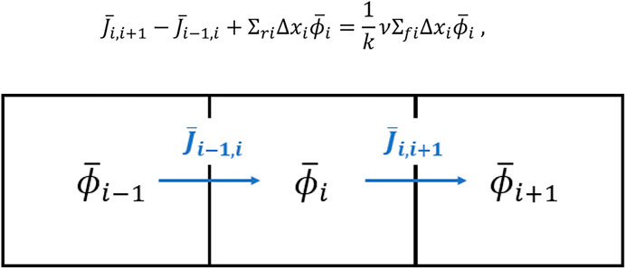
FIGURE 1. Balance within a node of interest.

The correction factor ${\widehat{D}}_{i,i+1}$ can be envisioned for Eq. 2 which alters the net current to be the reference current as follows:

${\overline{J}}_{i,i+1}^{ref}=-{\tilde{D}}_{i,i+1}\left({\overline{\varphi }}_{i+1}-{\overline{\varphi }}_i\right)-{\widehat{D}}_{i,i+1}\left({\overline{\varphi }}_{i+1}+{\overline{\varphi }}_i\right),(4)$

${\widehat{D}}_{i,i+1}=\frac{-{\tilde{D}}_{i,i+1}\left({\overline{\varphi }}_{i+1}-{\overline{\varphi }}_i\right)-{\overline{J}}_{i,i+1}^{ref}}{\left({\overline{\varphi }}_{i+1}+{\overline{\varphi }}_i\right)}.(5)$

The neutron balance equation, i.e., Eq. 1, is known to be a well-defined problem, in which a single solution (eigenvalue) exists for a certain current value. Hence, the inclusion of Eqs 4, 5 while implementing the FDM would provide an equivalent solution to that of the reference, which is exploited for acquiring ${\overline{J}}_{i,i+1}^{ref}$ (Smith, 1983). The simplicity of the FDM with its coarse node size will manifest as a reduction in the computing burden (acceleration), hence attaining the name of coarse-mesh finite difference (CMFD) method.

Partial Current–Based CMFD Method

It is apparent that the preservation of partial currents will guarantee retaining net current. From such a perspective, two correction factors for incoming and outgoing partial currents can be considered as depicted in Figure 2, attaining the name of partial current–based CMFD (pCMFD) method (Cho et al., 2003):

${\overline{J}}_{i,i+1}^{+ref}=-\frac{{\tilde{D}}_{i,i+1}\left({\overline{\varphi }}_{i+1}-{\overline{\varphi }}_i\right)+2{\widehat{D}}_{i,i+1}^{+}{\overline{\varphi }}_i}{2}(6)$

${\overline{J}}_{i,i+1}^{-ref}=\frac{{\tilde{D}}_{i,i+1}\left({\overline{\varphi }}_{i+1}-{\overline{\varphi }}_i\right)+2{\widehat{D}}_{i,i+1}^{-}{\overline{\varphi }}_{i+1}}{2}(7)$

FIGURE 2

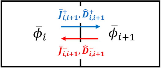
FIGURE 2. Visualization of pCMFD correction schemes.

The net current can be expressed as

${\overline{J}}_{i,i+1}^{ref}={\overline{J}}_{i,i+1}^{+ref}-{\overline{J}}_{i,i+1}^{-ref}=-{\tilde{D}}_{i,i+1}\left({\overline{\varphi }}_{i+1}-{\overline{\varphi }}_i\right)-\left({\widehat{D}}_{i,i+1}^{+}{\overline{\varphi }}_i+{\widehat{D}}_{i,i+1}^{-}{\overline{\varphi }}_{i+1}\right)(8)$

where

${\widehat{D}}_{i,i+1}^{+}=-\frac{{\tilde{D}}_{i,i+1}\left({\overline{\varphi }}_{i+1}-{\overline{\varphi }}_i\right)+2{\overline{J}}_{i,i+1}^{+ref}}{2{\overline{\varphi }}_i}(9)$

${\widehat{D}}_{i,i+1}^{-}=-\frac{{\tilde{D}}_{i,i+1}\left({\overline{\varphi }}_{i+1}-{\overline{\varphi }}_i\right)-2{\overline{J}}_{i,i+1}^{-ref}}{2{\overline{\varphi }}_{i+1}}(10)$

One-Node CMFD Method

The correction factors for the preservation of net current and surface flux could be introduced separately for each node as shown in Figure 3, where incoming partial current acts as a boundary condition for invoking kernel calculation (Shin and Kim, 1999). Such an approach differs from the conventional CMFD and pCMFD methods which introduce correction alongside two contiguous nodes:

${\overline{J}}_{i,i+1}=-\frac{2D_i}{\Delta x_i}\left({\overline{\varphi }}_s-{\overline{\varphi }}_i\right)-\frac{2{\widehat{D}}_i^R}{\Delta x_i}\left({\overline{\varphi }}_s+{\overline{\varphi }}_i\right)(11)$

${\overline{J}}_{i,i+1}=-\frac{2D_{i+1}}{\Delta x_{i+1}}\left({\overline{\varphi }}_{i+1}-{\overline{\varphi }}_s\right)-\frac{2{\widehat{D}}_{i+1}^L}{\Delta x_{i+1}}\left({\overline{\varphi }}_s+{\overline{\varphi }}_{i+1}\right)(12)$

FIGURE 3

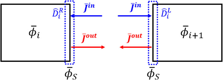
FIGURE 3. Visualization of one-node CMFD correction factors.

Equating Eqs 11, 12 yields the following expression for the surface flux:

${\overline{\varphi }}_s=\frac{\Delta x_{i+1}\left(D_i-{\widehat{D}}_i^R\right){\overline{\varphi }}_i+\Delta x_i\left(D_{i+1}+{\widehat{D}}_{i+1}^L\right){\overline{\varphi }}_{i+1}}{\Delta x_{i+1}\left(D_i+{\widehat{D}}_i^R\right)+\Delta x_i\left(D_{i+1}-{\widehat{D}}_{i+1}^L\right)}(13)$

where

${\widehat{D}}_i^R=-\frac{\Delta x_i {\overline{J}}_{i,i+1}^{ref}+2D_i\left({\overline{\varphi }}_s^{ref}-{\overline{\varphi }}_i\right)}{2\left({\overline{\varphi }}_s^{ref}+{\overline{\varphi }}_i\right)}(14)$

${\widehat{D}}_{i+1}^L=-\frac{\Delta x_{i+1} {\overline{J}}_{i,i+1}^{ref}+2D_{i+1}\left({\overline{\varphi }}_{i+1}-{\overline{\varphi }}_s^{ref}\right)}{2\left({\overline{\varphi }}_s^{ref}+{\overline{\varphi }}_{i+1}\right)}(15)$

Originally devised for parallel acceleration, the aforementioned acceleration scheme, which is referred to as one-node CMFD, can still be applied in a similar manner to that of the conventional CMFD or pCMFD method. Note that, for such an implementation, preservation of net current becomes irrelevant to surface flux values.

Nodal Expansion Method

As aforementioned, the underlying philosophy of CMFD-based acceleration is retaining current information from higher-order solutions, which is often the nodal calculation for whole-core analyses. In this work, the well-known nodal expansion method (NEM) was implemented as a kernel calculation, which is an assessment of current information and its corresponding correction factors for the neighboring two-node configuration. The correction factor is then considered during the formulation of discretized migration operator being analogous to that of the simple FDM, and the overall procedure is often referred to as NEM-CMFD calculation (Downar et al., 2009).

The detailed 1D flux and the transverse leakage term for a certain direction of interest are expanded via fourth-order and second-order polynomial basis functions (Legendre polynomials), respectively:

${\varphi }_g\left(\xi \right)=a_{g,0}{P}_0\left(\xi \right)+a_{g,1}{P}_1\left(\xi \right)+a_{g,2}{P}_2\left(\xi \right)+a_{g,3}{P}_3\left(\xi \right)+a_{g,4}{P}_4\left(\xi \right)(16)$

$L_g\left(\xi \right)=L_{g,0}{P}_0\left(\xi \right)+L_{g,1}{P}_1\left(\xi \right)+L_{g,2}{P}_2\left(\xi \right)(17)$

$P_0\left(\xi \right)=1, P_1\left(\xi \right)=\xi , P_2\left(\xi \right)={\xi }^2-\frac{1}{12} , P_3\left(\xi \right)={\xi }^3-\frac{1}{4}\xi , P_4\left(\xi \right)={\xi }^4-\frac{3}{10}{\xi }^2+\frac{1}{80}(18)$

where $\xi$ is the direction of interest, $a_{g,i}$ is the ith-order flux expansion coefficient for group g, and $L_{g,i}$ is the ith-order transverse leakage expansion coefficient for group g. The determination of net current then corresponds to calculation of flux expansion coefficients, where transverse leakage information must be pre-determined before invoking the NEM kernel calculation. Note that it is the presence of transverse leakage that complicates the assessment of direct-mathematical adjoint flux.

For a two-node NEM calculation, a total of 8G (G = number of groups) coefficients must be determined, which requires the same number of governing equations. Flux continuity (1G), current continuity (1G), and zeroth, first, and second moment node balance equations (2G for each) are envisioned for such a case, which results in a generation of 8G by 8G matrix equation. In contrast, a 4G by 4G matrix equation is formulated for a node at the boundary, where incoming partial current information is used in lieu of continuity equations.

Attributes of Numerical Adjoint Flux

Accompanied by proper usage of nodal kernel(s), either aided by transverse leakage or not, CMFD-based acceleration provides an FDM-like matrix where correction factors retain the net current information, rendering the solution to be that of the nodal calculation. The numerical adjoint can be readily calculated through the transpose of such a matrix representation; however, the correction factors manifest as a non-self-adjoint issue. Hence, the acquired numerical adjoint deviates from the reference one that possesses the self-adjoint property, where the extent of deviation depends on the type of CMFD acceleration scheme being utilized.

Self-Adjoint Issue

The multigroup diffusion equation can be written as follows:

$M_g{\varphi }_g=\frac{{\chi }_g}{k}{\displaystyle \sum }_{g\prime =1}^G\nu {\Sigma }_{f,g\prime }{\varphi }_{g\prime }+{\displaystyle \sum }_{\begin{array}{c}g\prime =1\\ \left(g\prime \ne g\right)\end{array}}^G{\Sigma }_{s,g\prime \to g}{\varphi }_{g\prime }(19)$

where G and k represent the number of energy groups and multiplication factor, $M_g$ denotes the migration operator for group g ($M_g{\varphi }_g:=-\nabla \cdot D_g\nabla {\varphi }_g+{\Sigma }_{r,g}{\varphi }_g$), and all the other notations are those of the convention. Note that, through proper discretization, the given equation can be represented in a matrix form. The numerical adjoint flux can then be calculated by transposing Eq. 19:

$M_g^{†}{\varphi }_g^{†}=\frac{1}{k}{\displaystyle \sum }_{g\prime =1}^G{\chi }_{g\prime }\nu {\Sigma }_{f,g}{\varphi }_{g\prime }^{†}+{\displaystyle \sum }_{\begin{array}{c}{g}^{\prime }=1\\ \left(g\prime \ne g\right)\end{array}}^G{\Sigma }_{s,g\to g\prime }{\varphi }_{g\prime }^{†}(20)$

where superscript dagger ($†$) signifies the adjoint operation.

Mathematically, it could be shown that the continuous migration operator for a certain group is self-adjoint (Ott and Neuhold, 1985). Such a feature is retained for the FDM approach, however, but not for the CMFD accelerated nodal calculation due to the presence of correction factors. The discretized balance equation can be generalized as follows:

$a_{i,i-1}{\overline{\varphi }}_{i-1}+a_{i,i}{\overline{\varphi }}_i+a_{i,i+1}{\overline{\varphi }}_{i+1}=s_i(21)$

where $a_{i,j}$ represents the contribution from ${\overline{\varphi }}_j$ for the neutron balance concerning ${\overline{\varphi }}_i$ and $s_i$ denotes the source term for node i containing both scattering and fission. Table 1 summarizes the matrix entries for the FDM and CMFD methods, where only the FDM approach retains the self-adjoint of the migration matrix, i.e., $a_{i-1,i}= a_{i,i-1}$ and $a_{i,i+1}= a_{i+1,i}$.

TABLE 1

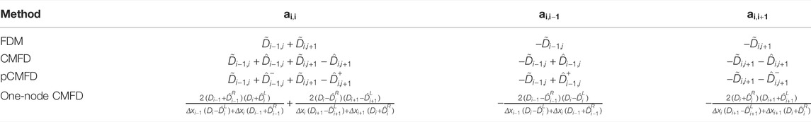
TABLE 1. Migration matrix entries for CMFD methods.

It could be observed that all the enumerated CMFD methods do not retain the self-adjoint property for the group-wise migration matrix. In addition, for the conventional CMFD and one-node CMFD, it could be easily shown that the absolute magnitude of corrections factors will dwindle with a decrease in the mesh size, i.e., numerators for Eqs 5, 14, and 15 converge to zero:

$-{\tilde{D}}_{i,i+1}\left({\overline{\varphi }}_{i+1}-{\overline{\varphi }}_i\right)\to {\overline{J}}_{i,i+1}^{ref}(22)$

$-\frac{D_i}{\Delta x_i/2}\left({\overline{\varphi }}_s^{ref}-{\overline{\varphi }}_i\right)\to {\overline{J}}_{i,i+1}^{ref}(23)$

However, correction factors for pCMFD do not converge to zero like the other two CMFD-based acceleration schemes:

$\begin{array}{l}{\widehat{D}}_{i,i+1}^{+}=-\frac{{\tilde{D}}_{i,i+1}\left({\overline{\varphi }}_{i+1}-{\overline{\varphi }}_i\right)+2{\overline{J}}_{i,i+1}^{+ref}}{2{\overline{\varphi }}_i}\\ \cong \frac{J_{i,i+1}^{ref}-2{\overline{J}}_{i,i+1}^{+ref}}{2{\overline{\varphi }}_i}=\frac{\left({\overline{J}}_{i,i+1}^{+ref}-{\overline{J}}_{i,i+1}^{-ref}\right)-2{\overline{J}}_{i,i+1}^{+ref}}{2{\overline{\varphi }}_i}=-\frac{{\overline{J}}_{i,i+1}^{+ref}+{\overline{J}}_{i,i+1}^{-ref}}{2{\overline{\varphi }}_i}.\end{array}(24)$

The inclusion of correction factors can be expressed in the following manner:

$\left(M+\delta M_1+\delta M_2\right){\varphi }_{CMFD}=\frac{1}{k}F{\varphi }_{CMFD}(25)$

where ${\varphi }_{CMFD}$ represents the CMFD-based flux and $\delta M_1$ and $\delta M_2$ denote diagonal and off-diagonal correction entries, respectively. The transpose of Eq. 25 can be written as

$\left(M^{†}+\delta M_1^{†}+\delta M_2^{†}\right){\varphi }_{CMFD}^{†}=\frac{1}{k}{F}^{†}{\varphi }_{CMFD}^{†}(26)$

Since the diagonal matrix is self-adjoint, i.e., $\delta M_1=\delta M_1^{†}$, subtraction of the two equations above garners

$\left(M+\delta M_1\right)\left({\varphi }_{CMFD}-{\varphi }_{CMFD}^{†}\right)+\left(\delta M_2{\varphi }_{CMFD}-\delta M_2^{†}{\varphi }_{CMFD}^{†}\right)=\frac{1}{k}F\left({\varphi }_{CMFD}-{\varphi }_{CMFD}^{†}\right).(27)$

If $\delta M_2\cong \delta M_2^{†}$ is satisfied, ${\varphi }_{CMFD}={\varphi }_{CMFD}^{†}$ becomes the solution for Eq. 27, which corresponds to the preservation of self-adjoint feature.

Since CMFD-induced and one-node CMFD–induced correction factors converge to zero with an increase in the number of nodes, their corresponding numerical adjoints would also converge to the reference, which is not expected for the pCMFD-based numerical adjoint flux.

Negative Adjoint Flux Issue

The correction factors in the discretized balance equation could result in the occurrence of negative numerical adjoint flux values as pointed out in previous studies which implemented the analytic nodal method (ANM) while deducing correction factors (Müller, 2014). Such an anomaly ensues when the off-diagonal and its corresponding diagonal entry of the migration matrix attain the same sign, which cannot be prevented for the conventional CMFD method. To circumvent such an issue, a different formula for net current preservation can be partially utilized under certain conditions; however, such an approach deteriorates the consistency in the CMFD formulation, i.e., ad hoc up to a certain extent.

Recalling that the usage of one-node CMFD in a two-node manner, i.e., not parallelized, could preserve the net current regardless of its surface flux values, one could exclude the occurrence of negative adjoint flux values through proper adjustment of the surface flux values. It is noteworthy to articulate that consistent usage of the same surface flux value while formulating the correction factors is responsible for the preservation of the current.

From Eqs 14, 15, it could be recognized that the one-node CMFD correction factors have the same unit as the diffusion coefficient. Since it is unphysical for the correction factor–included diffusion coefficient to be negative, the following conditions can be envisioned:

${\overline{\varphi }}_s^{ref}\le \frac{\Delta x_i}{4D_i}\left|{\overline{J}}_{i,i+1}^{ref}\right|(28)$

${\overline{\varphi }}_s^{ref}\le \frac{\Delta x_{i+1}}{4D_{i+1}}\left|{\overline{J}}_{i,i+1}^{ref}\right|(29)$

Eqs 28, 29 represent the criterion for correction factors ${\widehat{D}}_i^R$ and ${\widehat{D}}_{i+1}^L$ being less than their associated diffusion coefficient in magnitude, respectively. Through adjustment of surface flux to suffice Eqs 28, 29, the occurrence of negative numerical adjoint flux can be stifled.

Numerical Results

One-Group Reactor Problem

To test the deviation in the self-adjoint feature for various CMFD-based numerical adjoint fluxes, a simple one-group two-dimensional reactor problem was considered as shown in Figure 4. Two types of assemblies with a length of 20 cm are considered as shown in the cartoon, where their cross-section (XS) values are enumerated in Table 2.

FIGURE 4

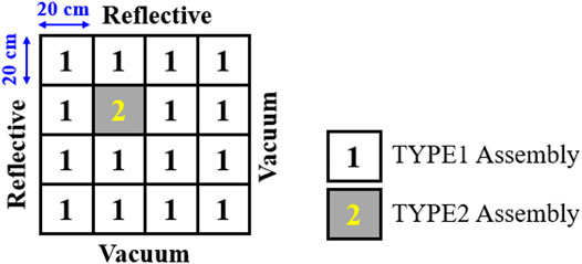
FIGURE 4. One-group reactor problem.

TABLE 2

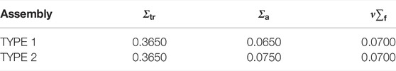
TABLE 2. Cross-section (XS) for the one-group reactor problem.

For the acquisition of numerical adjoints, the nodal expansion method (NEM) kernel was utilized, whereas the reference adjoint flux was obtained via the FDM while dividing each assembly into equally spaced 2,500 nodes (50 × 50 per assembly). Since the FDM-based numerical adjoint always retains the self-adjoint feature, the acquired fine node-based result was regarded as a reference after condensing into an assembly-wise value according to the following equation (Downar et al., 2009):

${\displaystyle \underset{0}{\overset{\infty }{\int }}dE}{\displaystyle \underset{V}{\int }dV{\varphi }^{†}}\left(\mathit{r},E^{\prime }\right)\varphi \left(\mathit{r},E^{\prime }\right) =1.0(30)$

The acquired multiplication factors for both forward and adjoint calculations are given in Table 3, where all the cases exhibit the same value.

TABLE 3

TABLE 3. Calculated multiplication factors for the one-group reactor problem.

Figure 5 illustrates the acquired adjoint fluxes from each acceleration scheme, where normalization according to Eq. 30 was performed for comparison. It could be recognized that only the pCMFD-based numerical adjoint flux exhibits a different distribution. Figure 6 summarizes the calculation result where the absolute value of percentage error for each case is given for both forward and adjoint fluxes. Note that the numerical adjoint flux exhibits the most conspicuous error for the TYPE 2 assembly region due to its enlarged absorption XS value:

$ERR(\%)=\left|\frac{{\varphi }^{ref}-{\varphi }^{CMFD}}{{\varphi }^{ref}}\right|\times 100.(31)$

FIGURE 5

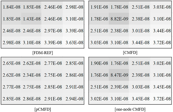
FIGURE 5. CMFD-based numerical adjoint fluxes.

FIGURE 6

FIGURE 6. Percentage error for forward and adjoint fluxes with a node size of 20 cm.

As aforementioned, the deviation from the self-adjoint feature weakens as the size of the node dwindles. A similar analysis was performed by imposing a node size of 10 cm, where reduction in the adjoint flux error is observed for both CMFD and one-node CMFD (1NCMFD) cases as depicted in Figure 7.

FIGURE 7

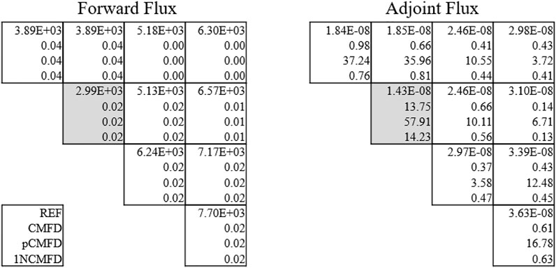
FIGURE 7. Percentage error for forward and adjoint fluxes with a node size of 10 cm.

KWU 2D Benchmark Problem

The KWU PWR 2D benchmark problem has been considered while excluding the presence of soluble boron under fully rodded conditions (Benchmark Source Situation, 1985). The configuration of the reactor problem is given in Figure 8 alongside four different positions for imposing localized perturbation in the absorption XS.

FIGURE 8

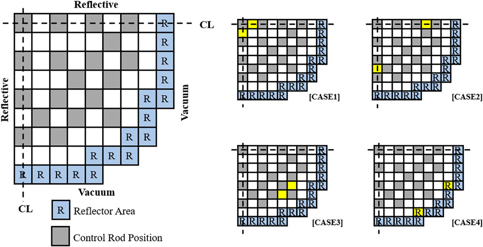
FIGURE 8. KWU 2D core configuration.

The attainment of reference adjoint flux was done in a similar fashion to that of one-group reactor problem while dividing each assembly into equally spaced 10,000 nodes (100 × 100 per assembly). Table 4 juxtaposes the calculated multiplication factors, where the same values are obtained regardless of the CMFD acceleration schemes as expected. Note that each assembly was taken as a single node during the CMFD accelerated nodal calculation.

TABLE 4

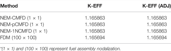
TABLE 4. Calculated multiplication factors for the KWU 2D problem.

The acquired numerical adjoint fluxes for both fast and thermal groups are shown in Figures 9, 10, where pCMFD-based results do not conform with the other results. In addition, negative adjoint flux values (red color) are observed for the thermal group adjoint flux in the peripheral regions as depicted in Figure 10, where the surface flux attained from the NEM kernel calculation was directly utilized for one-node CMFD acceleration, i.e., no correction was made for acquisition of correction factors.

FIGURE 9

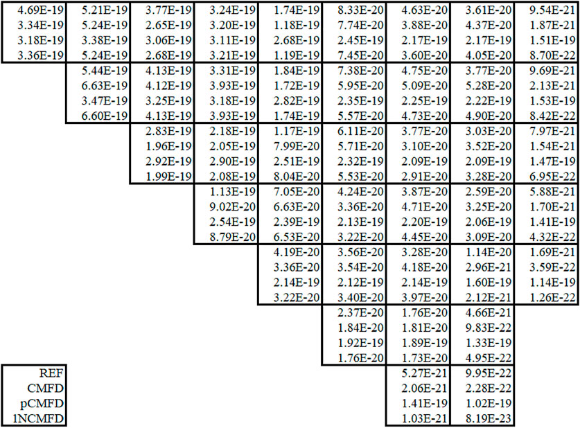
FIGURE 9. Fast group numerical adjoint flux for the KWU 2D problem.

FIGURE 10

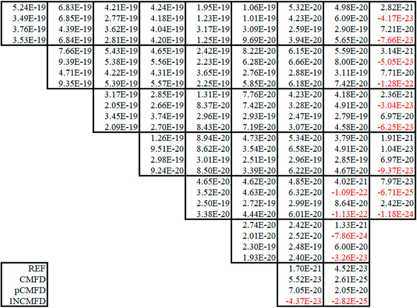
FIGURE 10. Thermal group numerical adjoint flux for the KWU 2D problem.

In order to stifle the occurrence of negative adjoint flux as shown in Figure 10, the surface flux was adjusted as follows to alter the correction factor to be zero when one of Eqs 28, 29 is met during a one-node CMFD calculation. The resulting numerical adjoint is illustrated in Figures 11, 12, where no negative values are observed:

${\overline{\varphi }}_s^{ref}=-\frac{1}{2}\cdot \frac{\Delta x_i {\overline{J}}_{i,i+1}^{ref}}{D_i}+{\overline{\varphi }}_i for {\widehat{D}}_i^R(32)$

${\overline{\varphi }}_s^{ref}=\frac{1}{2}\cdot \frac{\Delta x_{i+1} {\overline{J}}_{i,i+1}^{ref}}{D_{i+1}}+{\overline{\varphi }}_{i+1} for {\widehat{D}}_{i+1}^L(33)$

FIGURE 11

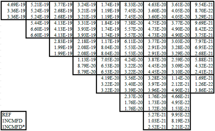
FIGURE 11. One-node CMFD–based fast group numerical adjoint flux for the KWU 2D problem. The adjusted result is denoted with an asterisk (*).

FIGURE 12

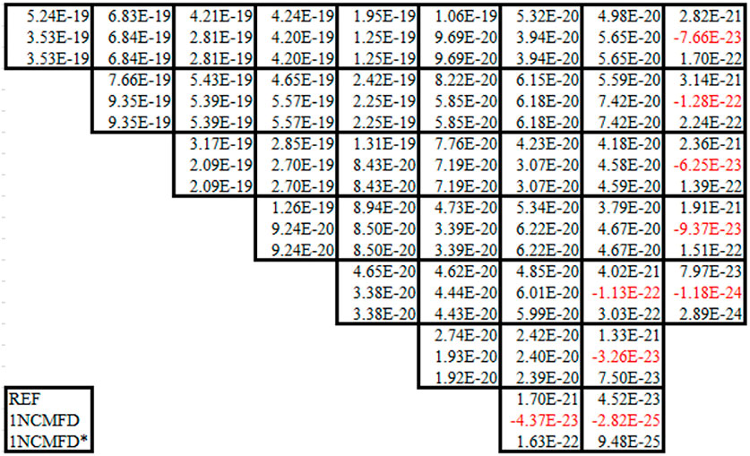
FIGURE 12. One-node CMFD–based thermal group numerical adjoint flux for the KWU 2D problem. The adjusted result is denoted with an asterisk (*).

For a systematic comparison between the numerical adjoint fluxes, the first-order perturbation theory was utilized, where assessment in the change of reactivity was made and compared with the reference value. Note that the reference reactivity change was evaluated via a direct solution of the perturbed system. The reactivity change can be estimated as follows:

$\Delta \rho =\frac{{\displaystyle \underset{0}{\overset{\infty }{\int }}{\displaystyle \underset{V}{\int }dEdV{\varphi }_0^{†}\left(\mathbf{r},E\right)}\left({\lambda }_0\Delta \mathbf{F}-\Delta \mathbf{M}\right)}{\varphi }_0\left(\mathit{r},E\right)}{{\displaystyle \underset{0}{\overset{\infty }{\int }}{\displaystyle \underset{V}{\int }dEdV{\varphi }_0^{†}\left(\mathbf{r},E\right)}{\mathbf{F}}_0}{\varphi }_0(\mathbf{r},E)}(34)$

where $\lambda$ denotes the reciprocal of multiplication factor, $F$ and $M$ represent augmented fission and migration operators, respectively, and all the other notations are those of the convention.

Four different perturbation scenarios are envisaged as shown in Figure 8, where a change in the absorption XS was locally imposed (yellow colored assemblies). The extent of variation in the XS compared to its original value was set to be 30% for cases 1 to 3 and 80% for case 4. Two different adjoint fluxes are considered for the one-node CMFD method, namely, the original and the adjusted one. Note that the former result is subjected to a negative value issue. The calculated results are enumerated from Tables 5–8.

TABLE 5

TABLE 5. Reactivity change (pcm) estimation for perturbation case 1.

TABLE 6

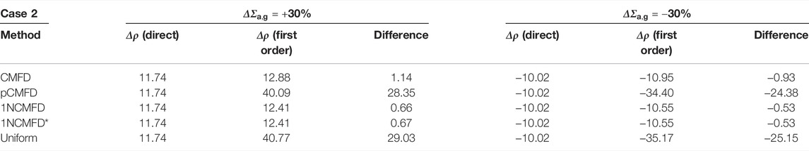
TABLE 6. Reactivity change (pcm) estimation for perturbation case 2.

TABLE 7

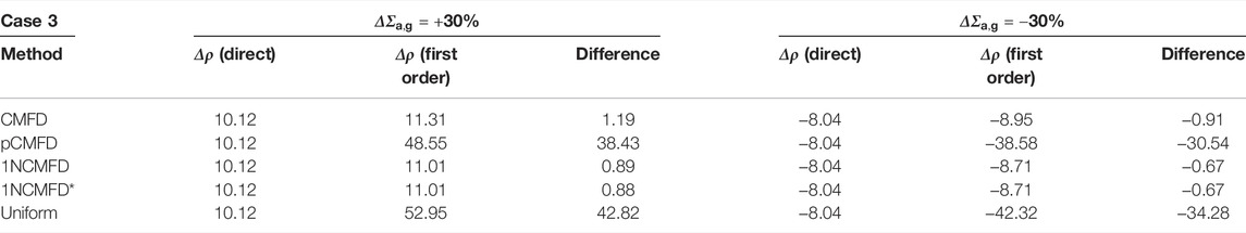
TABLE 7. Reactivity change (pcm) estimation for perturbation case 3.

TABLE 8

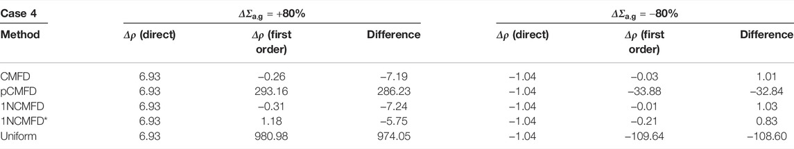
TABLE 8. Reactivity change (pcm) estimation for perturbation case 4.

Where the asterisk denotes the adjusted one-node CMFD numerical adjoint and UNIFORM indicates the usage of unit vector while estimating reactivity change according to the first-order perturbation theory. It could be observed that the exploitation of one-node CMFD–based adjoint flux renders the estimation to be more accurate compared to other approaches. Especially, for the perturbation in the reflector region, i.e., case 4, only the negative adjoint flux issue–resolved one-node CMFD exhibits a reliable result.

Conclusion

In this work, attributes of numerical adjoint fluxes that are obtained from various CMFD-based acceleration methods, e.g., conventional CMFD, pCMFD, and one-node CMFD, are investigated alongside a thorough mathematical description. It is noteworthy to mention that one-node CMFD formulation was employed under the two-node configuration, i.e., not in a parallelized manner. With the exploitation of the NEM kernel, the CMFD correction factors that are introduced in the migration operator matrix render such a matrix to be non-self-adjoint for all the presented CMFD acceleration schemes. Especially, it was found that the pCMFD-based numerical adjoint flux cannot retain the self-adjoint feature of a migration operator regardless of its mesh size, insinuating its inherent limitation for acquiring a reliable estimation for adjoint information. In addition, the occurrence of negative adjoint flux values was encountered for both conventional CMFD and one-node CMFD methods, which result in an erroneous reactivity estimation when employed as a weighting function for the first-order perturbation theory.

Mathematically, the preservation of net current information is independent of the choice of surface flux value if it is consistently applied for the generation of correction factors regarding the one-node CMFD method under the two-node configuration. Nevertheless, the magnitude of such correction factors, which has a unit of length, must not exceed the given diffusion coefficient to prevent encountering negative adjoint flux values. Hence, an adjustment scheme in the surface flux to circumvent such an issue while deducing the correction factors was proposed regarding the one-node CMFD method. A systematic analysis based on the first-order perturbation theory vividly attests to the effectiveness of employing the adjusted one-node CMFD–based numerical adjoint flux concerning a localized perturbation where a negative adjoint flux originally appeared. The stability analysis for the proposed surface flux–adjusted one-node CMFD acceleration scheme will be deliberated in the near future.

Data Availability Statement

The original contributions presented in the study are included in the article/Supplementary Material, and further inquiries can be directed to the corresponding author.

Author Contributions

TO wrote the first draft of the manuscript. TO and YK contributed to conception and design of the study. YK provided overall supervision.

Funding

This work was supported by the National Research Foundation of Korea Grant funded by the Korean government (NRF-2016R1A5A1013919) and BK21 FOUR (Fostering Outstanding Universities for Research; project No. 4120200313637).

Conflict of Interest

The authors declare that the research was conducted in the absence of any commercial or financial relationships that could be construed as a potential conflict of interest.

Publisher’s Note

All claims expressed in this article are solely those of the authors and do not necessarily represent those of their affiliated organizations, or those of the publisher, the editors, and the reviewers. Any product that may be evaluated in this article, or claim that may be made by its manufacturer, is not guaranteed or endorsed by the publisher.

References

Benchmark Source Situation (1985). Tech. Rep. ANL-7416. Argonne, IL: National Energy Software Center.

Google Scholar

Cho, N. Z., Lee, G. S., and Park, C. J. (2003). On a New Acceleration Method for 3D Whole-Core Transport Calculations. Sasebo: Annual Meeting of the Atomic Energy Society of Japan.

Google Scholar

Downar, T., Xu, Y., and Seker, V. (2009). PARCS NRC Core Neutronics Simulator THEOTY MANUAL. Ann Arbor, MI.

Google Scholar

Hong, S. G., and Cho, N. Z. (1995). Mathematical Adjoint Solution to the Analytic Expansion Nodal (AFEN) Method. J. Korean Nucl. Soc. 27, 374–384.

Google Scholar

Lawrence, R. D. (1984). Perturbation Theory within the Framework of a Higher-Order Nodal Method. Trans. Am. Nucl. Soc. 46, 402.

Google Scholar

Lewins, J. (1965). ‘IMPORTANCE: The Adjoint Function’. Oxford: Pergamon Press.

Google Scholar

Müller, E. (2014). On the Non-uniqueness of the Nodal Mathematical Adjoint. Ann. Nucl. Energ. 64, 333–342. doi:10.1016/j.anucene.2013.10.019

CrossRef Full Text | Google Scholar

Ott, K. O., and Neuhold, R. J. (1985). Introductory Nuclear Reactor Dynamics. American Nuclear Society.

Google Scholar

Shin, H. C., and Kim, Y. (1999). A Nonlinear Combination of CMFD and FMFD Methods. Pohang: Proceedings of Korean Nuclear Society Spring Meeting.

Google Scholar

Smith, K. S. (1983). Nodal Method Storage Reduction by Nonlinear Iteration. Trans. Am. Nucl. Soc. 44, 265.

Google Scholar