Research on the Amplitude–Phase Motion Equation for the Modeling of Wind Power System

The increasing penetration of wind power together with its high volatility could significantly impact the transient stability of the power grid. To quickly evaluate this impact, current engineering practice is primarily relying on time-domain simulation, which is computationally expensive despite that the results are more accurate. To solve this computational complexity issue, the amplitude–phase motion method is proposed to establish the electromechanical transient simulation model of the double-fed induction generator (DFIG) for wind energy. However, the traditional amplitude–phase motion equation (APME) suffers from the instability control from the abrupt change of terminal voltage induced by the system changes or flickers. To improve the transient stability of DFIG, this study firstly incorporates the q-axis current together with the amplitude change of terminal voltage into the phase error of the phase-locked loop (PLL). Then, the output phase of the terminal voltage of DFIG is highly combined with the q-axis current and the amplitude of terminal voltage to improve the internal control effect of the typical APME. The simulation results in the four-machine two-area power system with one wind farm demonstrate that the proposed method is able to maintain a stable operation of the wind farm and the power grid when experiencing a sharp disturbance of wind speed.

1 Introduction

To achieve a sustainable energy system of the future, it is imperative to integrate more variable renewable energy, such as wind and solar, and other new energy sources into the power grid. High wind power permeability is the development trend under the requirement of emission reduction and green energy. The installed wind power capacity was 330 million kW in China in 2021 (Yan et al., 2021). The wind turbines are connected to the grid through power-electronic converters, which results in the low inertia compared to the traditional power system with dominantly fossil fuel–driven generators. Therefore, the power system experiences much more extended swing under contingencies, which degrades the stability margin. Another significant issue resulting from the power-electronics–based power system is harmonic oscillation (Ebrahimzadeh et al., 2019). Compared to the PSS and AVR for traditional synchronous generators with a time constant of seconds, power converters for wind and solar are modulated in ns, which provides much faster dynamics and causes multiple time-scale control problems in the power system (Yuan et al., 2017). Therefore, the traditional modeling method of power system stability analysis may not be able to capture these emerging issues from power-electronic dominant power grids with renewables. It is in an urgent need to study the operational characteristics of power-electronic grid–connected renewables and provide theoretical support to maintain a stable operation of the power system with high penetration of new energy.

For the transient stability of the power system under high wind power penetration, it is important to establish a low-order, accurate, and open model (Zhang et al., 2017). The modeling analysis methods can be divided into three categories generally: the eigenvalue analysis method based on the state space theory, the impedance analysis method, and the amplitude–phase motion equation method. The eigenvalue analysis is a time-domain analysis method based on the state space, which is used to analyze the small signal stability in traditional power systems (Wang and Blaabjerg, 2019). The results are accurate while imposing a high computational complexity in simulation (Zong et al., 2020; Liu et al., 2021; Wu et al., 2021). The impedance method regards each device in the power system as an impedance, which can be characterized by its voltage and current. In this method, the grid and the generator are regarded as the combination of ideal source and impedance, respectively. Usually, the Nyquist criterion is used to determine the stability of power systems (Wen et al., 2016; Yan et al., 2016; Gao et al., 2018; Duan and Sheng, 2019). These models are simple in principle and easy to implement for analysis (Arabi et al., 2000). However, the impedance must be recalculated under different operation conditions. Moreover, the generator side cannot be regarded as a current source model if the output impedance of the generator is not large enough (Sun, 2011). It lacks the connection among key physical states in the dynamic process, so it is difficult to be applied to analyze dynamic problems at multiple time scales for large-scale power systems (Yuan et al., 2016).

How to keep the clear description of system characteristics without sacrificing the computation speed has always been the pursued goal. When the dynamic process of the power system suffers a disturbance, the power on each component will be changed to achieve a new balance by regulating the amplitude and phase of voltage as well. By the amplitude–phase motion equation method, the clear description between power imbalance and system states can be constructed (Yang et al., 2020), by simplifying the external characteristics into the amplitude and phase changes of voltage (Huang et al., 2019). In nature, by changing the voltage amplitude and phase, the amplitude and phase motion equation reproduces the system characteristics from the view of power balance between the input and the output of the whole system, which is explicit in the physical meaning and is simpler in modeling.

The modeling of DFIG has been realized in many research studies. Both the impendence method and the amplitude–phase method have analyzed the small signal dynamical behavior of power systems focusing on the different input–output relation. Through analysis, He et al. (2019) have concluded that the amplitude and phase motion equation of a single-machine infinite-bus system is similar to the classical second-order swing equation for a synchronous generator connected to an infinite bus, which supports the application of amplitude and phase motion equation in a dynamic process. This method applies to a wide range of scenarios, such as multi-input multi-output models and new perspective of equivalent system. The multi-input multi-output model is regarded as a single-input single-output equivalent model on the current time scale, and its voltage amplitude and phase dynamics are analyzed, respectively, in the study of Li et al. (2019). In the study of Zhao et al. (2018), the rotation of the rotor and the voltage of the capacitor are regarded as a real dynamical system, and the relationship between power balance and voltage change has been analyzed from the perspective of the component voltage vector. The vector controls have been proposed to solve the multiple time-scale problems of the electronic power system. In the study of Zhang et al. (2018), a frequency modulation method based on the phase motion equation has been proposed, and a typical phase-locked loop (PLL) synchronous vector control has been used to solve the problem of islanding. The time-scale problems of DC voltage control of the power system with the voltage source converter (VSC) connected to the grid have been studied by Yuan and Yuan (2018). The vector controls, including the DC voltage control, the phase-locked loop control, and the terminal voltage control, have been introduced to effectively replace the detection of VSC terminal voltage with the output power.

The angle stability has been realized to be a crucial factor that affects the stability of the power system. A typical APME model for the DFIG is proposed by Zhang et al. (2017), based on which the phase information has been added into the current-limiting control module by a feedback control loop. However, considering that the decrease of the voltage amplitude or the flicker of terminal phase affects the phase in the PLL and changes the dynamics of phase in the terminal voltage, a terminal voltage feedback control is further introduced into the DFIG model, which will make the change of terminal voltage phase closer to the real scenarios. Then, an improved APME model is established, and three cases are analyzed, including the steady-state process, the load changes, and the wind changes. The results show that the improved APME model does not change sharply with the change of wind speed.

2 Operation Characteristic of DFIG

A typical DFIG model is shown in Figure 1A. The stator side is directly connected to the grid through a transformer, while the rotor side is connected to the grid through an alternative current (AC)–direct current (DC)–alternative current (AC) converter. The control of DFIG mainly depends on the rotor side controller and the grid side controller. In general, the active power and reactive power of DFIG are mainly controlled to maximize the utilization of wind energy at the rotor side. The controller on the grid side keeps the DC voltage constant by changing the modulation coefficient, which also keeps the input power and the current in the sinusoidal waveform.

FIGURE 1

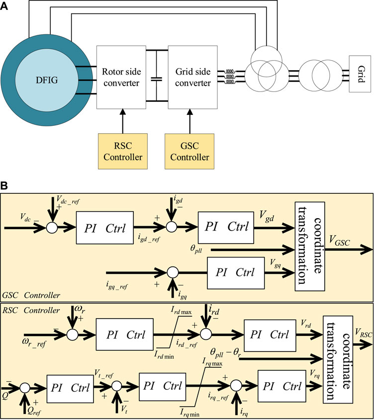
FIGURE 1. (A) Typical DFIG model. (B) Control module of the typical DFIG model.

Figure 1B is the GSC/RSC controller of the typical DFIG model. The active and reactive power is calculated by the terminal voltage and its current. The PLL controller samples phase information from terminal voltage, and this phase information combining with frequency obtained by the PLL controller is the basis for establishing the dq coordinate. The system is decoupled in the dq coordinate. The power system after decoupling can be more convenient for analysis and control. The active power can be controlled independently by adjusting the q-axis current of rotor, while the reactive power can be controlled independently by the d-axis current of rotor. Figure 1B shows a method to decouple the system. In the GSC controller module, the DC voltage V_dc between two converters, grid side current i_gd, and phase of PLL θ_pll are used to control the voltage of grid side converter V_GSC. In the RSC controller module, the reactive power Q, terminal voltage V_t, rotor speed ω_r, rotor current i_rd/i_rq, and the error between the phase of PLL and the phase of rotor θ_pll -θ_r are used to control the voltage of rotor side converter V_RSC.

The DFIG is a strongly coupled system because of the flux between stator windings and rotor windings. There exists a rotor magnetic field while three-phase AC is acting on the rotor windings. This field cuts the stator windings to produce the induced three-phase current. In return, the field produced by AC on stator windings also influences the current on rotor windings by changing its magnitude and phase. Thus, there are mutual constraints among stator current, rotor current, and stator voltage. The electromagnetic torque equation, active power equation, and reactive power equation are listed as the following equation, in which both components on the dq-axis have effects on power and torque:

$\{\begin{array}{l}{P}_s=\frac{3}{2}\mathrm{Re}\left(\stackrel{\rightharpoonup }{u_{sdq}}\stackrel{\rightharpoonup }{i_{sdq}^{\ast }}\right)=\frac{3}{2}\left(u_{sd}{i}_{sd}+u_{sq}{i}_{sq}\right),\\ Q_s=\frac{3}{2}\mathrm{Im}\left(\stackrel{\rightharpoonup }{u_{sdq}}\stackrel{\rightharpoonup }{i_{sdq}^{\ast }}\right)=\frac{3}{2}\left(u_{sq}{i}_{sd}-u_{sd}{i}_{sq}\right),\\ T_e=\frac{3}{2}{n}_p\left({\text{Ψ}}_{sd}{i}_{sq}-{\text{Ψ}}_{sq}{i}_{sd}\right)=\frac{3}{2}{n}_p\left({\text{Ψ}}_{rq}{i}_{rd}-{\text{Ψ}}_{rd}{i}_{rq}\right)\\ \begin{array}{c}\begin{array}{cc}& =\frac{3}{2}{n}_p{L}_m\left(i_{sq}{i}_{rd}-i_{sd}{i}_{rq}\right)\end{array}\end{array},\end{array}(1)$

where $P_s$ is the active power; $Q_s$ is the reactive power; s is the electromagnetic torque; $u_{sdq}$ is the stator dq-axis voltage; $i_{sdq}$ is the stator dq-axis current; ${\Psi }_{sd}$ represents the component of flux on the d-axis; ${\Psi }_{sq}$ represents the component of flux on the q-axis; $n_p$ is the number of pole-pairs; and $L_m$ is the mutual inductance between the stator and the rotor.

The vector control (VC) method is the core control method of DFIG, which can decouple their relationship and make the control of DFIG simpler. In the VC method, the stator current is transformed into dq-axis current on dq coordination. If the stator flux linkage is chosen as the d-axis, the components of stator flux can be written as Eq. 2 and the voltages on the dq-axis are shown as Eq. 3:

$\{\begin{array}{l}{\text{Ψ}}_{sd}=\left|{\text{Ψ}}_{sdq}\right|={\text{Ψ}}_s,\\ {\text{Ψ}}_{sq}=0,\end{array}(2)$

$u_{sd}=0,u_{sq}=U_s={\omega }_1{\text{Ψ}}_s,(3)$

where ${\Psi }_s$ is the magnitude of stator flux; ${\text{Ψ}}_{sdq}$ is the vector of stator flux space; and ${\omega }_1$ is the velocity of synchronous angular.

The electromagnetic torque equation can be simplified as Eq. 4, in which the magnitude of torque is only determined by the stator flux on the d-axis and rotor current on the q-axis. The stator flux on the d-axis is almost a constant here, so the rotor current on the q-axis can dominate the magnitude of electromagnetic torque. The active and reactive power can be simplified as Eq. 5. Equation 5 is further simplified as Eq. 7 by Eq. 6. Under the condition that the stator flux remains unchanged, the active power is only determined by the rotor current on the q-axis and the reactive power is mainly determined by the rotor current on the d-axis:

$T_e=\frac{3}{2}{n}_p\left({\text{Ψ}}_{sd}{i}_{sq}-{\text{Ψ}}_{sq}{i}_{sd}\right)=-\frac{3}{2}{n}_p\frac{L_m}{L_s}{\text{Ψ}}_s{i}_{rq},(4)$

$\{\begin{array}{l}{P}_s=\frac{3}{2}{u}_{sq}{i}_{sq}=\frac{3}{2}{U}_s{i}_{sq},\\ Q_s=\frac{3}{2}{u}_{sq}{i}_{sd}=\frac{3}{2}{U}_s{i}_{sd},\end{array}(5)$

$\{\begin{array}{l}{i}_{sd}=\frac{L_m}{L_s}\left(i_{ms}-i_{rd}\right),\\ i_{sq}=-\frac{L_m}{L_s}{i}_{rq},\end{array}(6)$

$\{\begin{array}{l}{P}_s=-\frac{3}{2}{\omega }_1{\text{Ψ}}_s\frac{L_m}{L_s}{i}_{rq},\\ Q_s=\frac{3}{2}{\omega }_1{\text{Ψ}}_s\frac{L_m}{L_s}\left(i_{ms}-i_{sd}\right),\end{array}(7)$

where $L_s$ represents the inductance of stator windings and $i_{ms}$ is the field current of stator.

The time scale of the AC current control loop and the DC voltage control loop is quite faster than that of the electromechanical characteristics, so they have often been ignored in the conventional control. The GE model, ignoring the AC current control loop and the DC voltage control loop, uses the main characteristics to describe the system (Clark et al., 2010). Under the premise that the main characteristics of DFIG can be reflected in the electromechanical time scale, this model is simple and the results are accurate, while its order is lower. Therefore, the GE model has been widely used in power system simulation. Hence, the GE model is taken as an example to analyze the structure and the control mode of the wind turbine. The control block of the GE model is shown in Figure 2.

FIGURE 2

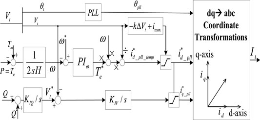
FIGURE 2. Control block of the GE model.

The rotating speed is calculated according to the electromagnetic torque and mechanical torque. Then, the reference value of the electromagnetic torque is calculated by the reference speed. The active current is given by the electromagnetic torque, speed, and the terminal voltage. The difference of reactive power is used to calculate the voltage reference. In the transient process, when the terminal voltage amplitude decreases, the active component of current will decrease due to the inertia, while the PI control will damp the collapse and increase the voltage by increasing the reactive current. Of course, the amplitude change of the terminal voltage will directly affect the active current, and the following equation gives its mathematical expression:

$i_{d-pll}^{\ast }=\{\begin{array}{c}{i}_{\max },\\ i_{\max }-k_v\text{Δ}{V}_t,\\ 0,\end{array}\begin{array}{cc}& \end{array}\begin{array}{c}\text{Δ}{V}_t<0\\ 0\le \text{Δ}{V}_t\le 0.4\\ 0.4\le \text{Δ}{V}_t\end{array}(8)$

where $i_{\max }$ is the maximum transient current of DFIG, whose value is set to 1.2 p.u. The control parameter $k_v$ is set to 3.05 by default, and $i_{d-pll}^{\ast }$ is the expected output of active current on the d-axis.

Considering that the voltage drop $\Delta V_t$ is within [0, 0.4 p.u.], and the voltage drop is 0.1 p.u., the following equation can be obtained:

$\text{Δ}{V}_t=0.9-V_t.(9)$

The spatial relationship on the dq-axis is shown in Figure 3.

FIGURE 3

FIGURE 3. dq-axis spatial relationship.

The transient current $i_{pll}$ of any phase and magnitude can be expressed by a combination of the dq-axis current amplitude and the phase output ${\theta }_{pll}$ of PLL. The transient current $i_{pll}$ is also a spatial vector, which can be expressed in the form of magnitude and phase. The dq-axis will rotate with the change of the frequency and phase of the terminal voltage, which can be obtained from the PLL block connected to the terminal of DFIG. After decomposing current $i_{pll}$ into two vertical components, the active and reactive power of DFIG can be controlled, respectively, through $i_q$ and $i_d$. Then, the spatial vector $i_{pll}$ is decomposed on the dq-axis for analysis and control:

$\{\begin{array}{c}{i}_d^2+i_q^2=i_{\text{pll}}^2,\\ {\theta }_{pll}=\arctan \frac{i_q}{i_d}.\end{array}(10)$

3 DFIG Model Construction Based on Amplitude–Phase Motion Equation

The idea of amplitude–phase motion equation is to construct its physical relationship through the change of the external input to the output. Physically, the object studied can be regarded as a black box. When the input power of the system is not balanced with the actual output power, the voltage of each component in the system will change in amplitude and phase, in order to achieve a new balance. Therefore, the model can reflect the dynamics of the external voltage amplitude and phase. Its physical nature is that the unbalanced power between the expected output and the actual output of the power system is embodied by the change of voltage amplitude and phase. Both the expected active power and reactive power are the reference values calculated by the control part.

Due to a large inertia of turbine, the electromechanical time scale with a time constant of 1 s is slow compared to the electromagnetic phenomenon (wind converter control is in ns). As the current time scale and voltage time scale are usually 0.01 and 0.1 s, respectively, it is assumed that the change and control of both the active power and the reactive power are instantaneous in the electromechanical time scale.

Since the actual output power of DFIG is the terminal voltage multiplied by the conjugate current, combined with Eqs 8–10, the actual outputs of active power and reactive power are calculated as follows:

$\begin{array}{l}\begin{array}{c}\end{array}P+jQ={\stackrel{\rightharpoonup }{V}}_t\ast {\overline{\stackrel{\rightharpoonup }{I}}}_{pll}=V_t{e}^{j{\theta }_t}\left(i_d^{\ast }-j{i}_q^{\ast }\right)e^{-j{\theta }_{pll}}\\ \begin{array}{c}\end{array}=V_t\left(i_d^{\ast }\cos {\theta }_{err}+i_q^{\ast }\sin {\theta }_{err}-j\ast i_q^{\ast }\cos {\theta }_{err}+j\ast i_d^{\ast }\sin {\theta }_{err}\right),\end{array}(11)$

where ${\theta }_{err}={\theta }_t-{\theta }_{pll}$; ${\overline{\stackrel{\rightharpoonup }{I}}}_{pll}$ represents the conjugation of the current phasor vector; ${\stackrel{\rightharpoonup }{V}}_t$ represents the phasor of the voltage vector; $i_d^{\ast }$ is the expected output of active current on the d-axis; $i_q^{\ast }$ is the expected output of reactive current on the q-axis; ${\theta }_t$ is the terminal voltage phase; ${\theta }_{pll}$ is the output phase of the PLL; and ${\theta }_{err}$ is the phase error of the PLL. In this expression, the parameters ${\theta }_{err}$, which have direct influences on the phase error of PLL, are determined by the terminal voltage phase and the output phase of the PLL. In the actual transient process, both the decrease of voltage amplitude and the flicker of voltage phase will affect the phase dynamics of DFIG. Hence, it is desired to improve the above expression for the improved transient performance by making ${\theta }_{err}$ directly respond to the change of terminal voltage amplitude. Meanwhile, phase dynamics also correlated with the variation of reactive current $i_q$. In this study, the expected reactive current on the q-axis is also deduced to construct the relationship with ${\theta }_{err}$, which is expressed as

$\begin{array}{l}P+jQ={\stackrel{\rightharpoonup }{V}}_t\ast {\overline{\stackrel{\rightharpoonup }{I}}}_{pll}=V_t{e}^{j{\theta }_t}\left(i_d^{\ast }-j{i}_q^{\ast }\right)e^{-j{\theta }_{pll}}\\ \begin{array}{ccc}& & \end{array}=V_t{e}^{j{\theta }_t}\left(i_d^{\ast }-j{i}_q^{\ast }\right)e^{j{\theta }_{pll}}{e}^{-2j{\theta }_{pll}}\\ \begin{array}{ccc}& & \end{array}=V_t{e}^{j{\theta }_t}\left(i_d^{\ast }-j{i}_q^{\ast }\right)e^{j{\theta }_{pll}}{e}^{-2j\arctan \frac{i_q^{\ast }}{i_d^{\ast }}},\end{array}(12)$

${\theta }_{err}={\theta }_t+{\theta }_{pll}-2\arctan \frac{i_q^{\ast }}{i_d^{\ast }}.(13)$

The active and reactive power can be obtained as

$P+jQ=V_t\left(i_d^{\ast }-j{i}_q^{\ast }\right)e^{j{\theta }_{err}}.(14)$

Furthermore, Euler’s formula $e^{ix}=\cos x+i\ast \sin x$ is used to expand Eq. 14 in order to observe the active and reactive power, respectively. The following results can be obtained:

$\begin{array}{l}P+jQ=V_t\left(i_d^{\ast }-j{i}_q^{\ast }\right)\left(\cos {\theta }_{err}+j\ast \sin {\theta }_{err}\right)\\ =V_t\left(i_d^{\ast }\cos {\theta }_{err}+i_q^{\ast }\sin {\theta }_{err}-j\ast i_q^{\ast }\cos {\theta }_{err}+j\ast i_d^{\ast }\sin {\theta }_{err}\right).\end{array}(15)$

Now, the unification of the right and left sides of the equation has been achieved. Both sides of the equation are complex numbers composed of real and imaginary parts. They can be further expressed as

$\left(\begin{array}{c}P\\ Q\end{array}\right)=V_t\left[\begin{array}{cc}\cos {\theta }_{err}& \sin {\theta }_{err}\\ \sin {\theta }_{err}& -\cos {\theta }_{err}\end{array}\right]\left[\begin{array}{c}{i}_d^{\ast }\\ i_q^{\ast }\end{array}\right].(16)$

It can be seen from Eq. 13 that the phase error ${\theta }_{err}$ of PLL is jointly determined by the actual terminal voltage phase, the phase on the phase-locked loop, and the expected current reference on the dq-axis. In the expression of ${\theta }_{err}$, the terminal voltage cannot be reflected directly. By using Eq. 15 and Eq. 16, d-axis current $i_d^{\ast }$ is deduced from the voltage amplitude. Furthermore, $i_d^{\ast }$ in Eq. 13 is replaced, and the terminal voltage amplitude is introduced into ${\theta }_{err}$, as shown in the following equation:

$i_d^{\ast }=i_{\max }-k_v\text{Δ}{V}_t=i_{\max }-k_v\left(0.9-V_t\right).(17)$

Then, ${\theta }_{err}$ is changed as

${\theta }_{err}={\theta }_t+{\theta }_{pll}-2\arctan \frac{i_q^{\ast }}{i_{\max }-k_v\left(0.9-V_t\right)},(18)$

where the amplitude of terminal voltage $V_t$ and the current $i_q$ are coupled into the phase error ${\theta }_{err}$ of PLL. From the perspective of control, the changes of terminal voltage amplitude and the q-axis current are fed to the phase dynamics of DFIG, by adding a feedback control to the typical model.

Figure 4 shows the derived amplitude–phase motion equation model based on the typical model of DFIG. The left side of the block diagram is the actual outputs of the active and reactive power of DFIG. The right end is the terminal voltage, and the middle is the control module based on the derivation equation above, in which there are the voltage control loops, the current control loops, and the phase deviation feedback loops from left to right.

FIGURE 4

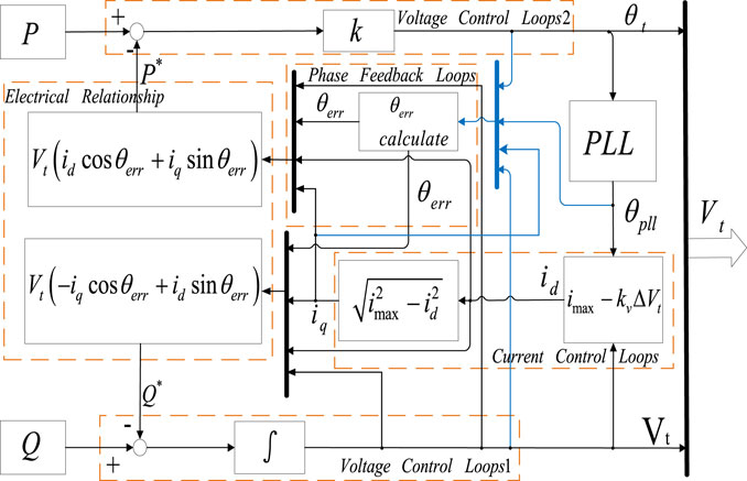
FIGURE 4. Improved amplitude–phase motion equation model.

4 Case Study

In order to verify the proposed optimization model, a typical IEEE benchmark case of a four-machine two-area power system with one wind farm has been established according to the schematic diagram in Figure 5, which has been analyzed and calculated by comparing the typical amplitude–phase motion equation model and the improved amplitude–phase motion equation model.

FIGURE 5

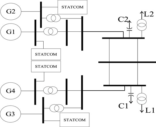
FIGURE 5. Four-machine two-area wind power system.

Figure 5 is further transformed to the block diagram of the four-machine two-area power system model (shown in Figure 6) for simulation. It consists of an improved amplitude–phase motion equation model of DFIG proposed in this paper and three traditional thermal generators. The generator G1 of the first subsystem is the optimization model based on the amplitude–phase motion equation, and the generator G3 of the third subsystem is the PV bus composed of the synchronous generator set. Generators G2 and G4 in the other two subsystems are PQ buses composed of the synchronous generators. The four generators in the power system are separated into four subsystems. In this part, the impedance modeling method is used to model the transmission network. According to the voltage and current relationship, each component is equivalent to a complex impedance model. The main components involved include the transmission lines, transformers, loads, and compensation capacitors. The general transmission line is equivalent to the complex impedance model, which is the combination of the resistance and reactance, while the long-distance transmission line is equivalent to the parallel form of the complex impedance and the capacitance admittance between the line and the ground. The transformer is equivalent to three complex impedances by a $\prod$ equivalent model. The compensation capacitor is equivalent to admittance $G+jB$. The loads, L1 and L2, are expressed as constant impedance models and are represented by the complex impedance.

FIGURE 6

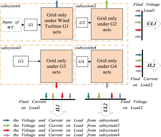
FIGURE 6. Block diagram of the four-machine two-area power system.

The simulation platform is shown in Figure 7. The four-machine two-area power system with the improved amplitude–phase motion equation is embedded in Figure 7B. In Figure 7A, an impeller and a blade that simulates the change of wind speed are used as the source of variable wind speed for the case study. The details are discussed in Section 4.2. In Figure 7B, the wind turbine control system includes the auxiliary power supply control, output display, and wind simulation unit. The terminal voltage and the current signals needed by the amplitude–phase motion equation model come from the output unit.

FIGURE 7

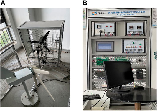
FIGURE 7. (A) Impeller of DFIG. (B) Wind turbine system.

Under the different operation conditions and with the different network structure parameters, the improved amplitude–phase motion equation is studied in the four-machine two-area power system model established here. At the same time, the performance of the four-machine two-area power system, with a typical amplitude–phase motion equation model, is given for comparison with the improved one under the same operation condition. And the advantages of the improved APME model are analyzed in this section.

4.1 Operation Condition I: Steady-State Process Simulation

The operating conditions are set as follows: the parameters of G1 are $P_1$ and $Q_1$, the parameters of two constant impedance loads in the system are $R_{L1}+j{X}_{L1}$ and $R_{L2}+j{X}_{L2}$, while $Y_{L1}$ and $Y_{L2}$ are the admittance of loads. The parameters of G2 are $V_{t2}$, $P_2$, and $Q_2$. The parameter of G3 is $U_3$, and the parameters of G4 are $V_{t4}$, $P_4$, and $Q_4$. In the steady-state simulation, there is no fault set. The values of each parameter are set as shown in Table 1.

TABLE 1

TABLE 1. Values of parameters.

Figure 8 is the voltage and current curve of the load in the power system with the improved APME model of DFIG, where IL1 represents the current passing through L1 and UL1 represents the voltage of L1. IL2 represents the current passing through L2, and UL2 represents the voltage of L2. It can be seen from Figure 8 that when the four-machine two-area power system has been started, the improved APME model has been regulated to reach a stable state very soon. The voltage and current in stabilization are within the reasonable range. The simulation result of the model is in line with the theoretical analysis of the power grid.

FIGURE 8

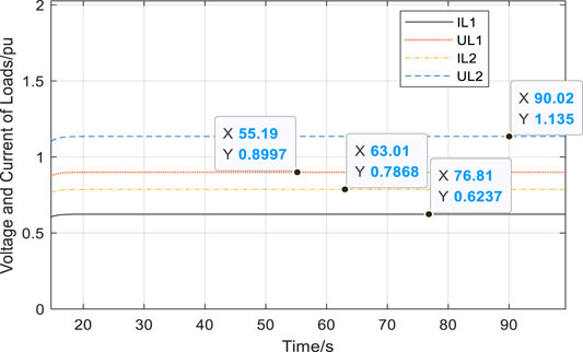
FIGURE 8. Voltage and current curves on load under operation condition I of the improved APME model.

Figure 9 displays the voltage and current curves of the load in the power system with a typical DFIG model. By comparing Figures 8, 9, it can be seen that the voltage and current curves of loads in the system reach a stable state quickly in both the improved and the typical model with a similar trend. The static parameters of loads are shown in Table 2. The difference of voltage and current before and after the DFIG model is improved is calculated.

FIGURE 9

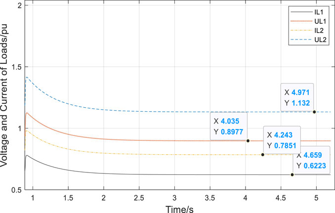
FIGURE 9. Voltage and current curves on load under operation condition I of the typical APME model.

TABLE 2

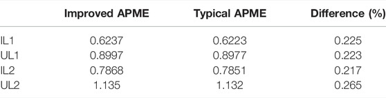
TABLE 2. Voltage and current details on loads under operation condition I.

The simulation results of the typical model are used as a reference to analyze the parameter difference of the two models, and the difference of current on L1 can be derived as

$IL{1}_{diff}=\left|\frac{IL{1}_{After}-IL{1}_{Before}}{IL{1}_{Before}}\right|\times 100\%.(19)$

The differences of the four parameters are all lower than 0.3%, which means that the steady-state process demonstrated by the two models under this set of parameters is basically the same. The improved APME model runs in line with the typical model under the same parameter setting. Its simulation performs the same as typical ones, without any fluctuation in the steady state, which verifies that the improved APME model is available under this group of parameter setting.

4.2 Operation Condition II: Impact of Wind Speed

Due to its randomness, the wind speed changes constantly with the change of temperature and air pressure, and gust wind may occur occasionally, which leads to shape changes of the speed. To simulate this change, the wind speed in a day is roughly divided into five periods: 2 m/s from 6 to 9 a.m., 4 m/s from 9 a.m. to 13 p.m., 6 m/s from 13 to 17 p.m., 8 m/s from 17 to 19 p.m., and 10 m/s after 19 p.m. All parameters are set to be the same as those in operation condition I, except the power injection from the DFIG.

Figure 10 shows the variation of voltage and current of the loads in the four-machine two-area power system, when wind speed changes with time mentioned above. As shown in Figure 10, the change of wind speed directly causes the output power change of DFIG, thus affecting the voltage and current of the load in the grid. When the wind speed changes suddenly, the voltage amplitude of loads does not change sharply, which indicates that the optimization model proposed in this paper has strong robustness and anti-interference ability.

FIGURE 10

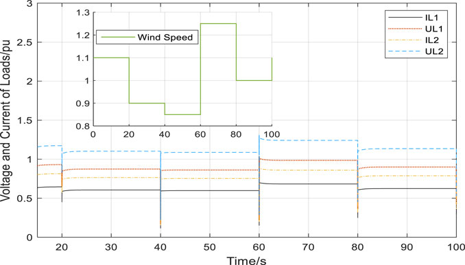
FIGURE 10. Voltage and current curves on load with wind speed change of the improved APME model.

In order to verify the model proposed in this paper, it is necessary to simulate the typical amplitude–phase motion equation of DFIG model under the same conditions. Figure 11 is the result of a typical model, without optimization control mentioned in this paper, in which the voltage and the current of the loads with the change of wind speed can be observed. The key parameters of simulation are set as follows: the variation of wind speed is divided into five sections, 1.1, 0.9, 0.85, 1.25, and 1 successively. The output power of the conventional generator G2 is $P_2=1,Q_2=-0.2$. The output voltage of G3 is 1 p.u., and the output power of the conventional generator G4 is $P_4=1,Q_4=0.2$. The value of two constant impedances in the power system is $Y_{L1}=Y_{L2}=0.4902-j0.4902$.

FIGURE 11

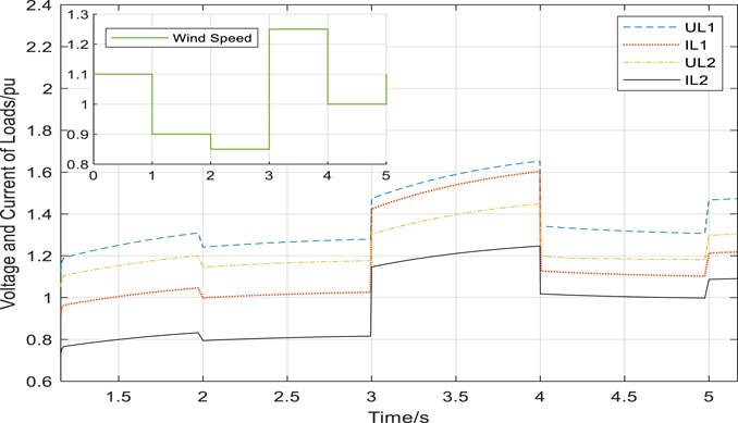
FIGURE 11. Voltage and current curves on load with wind speed change of the typical APME model.

The results show that the output voltage of DFIG follows the change of wind speed. Compared with the improved APME model, it is more sensitive to the change of wind speed. As such, it is concluded that its robustness is not as strong as the improved model. Actually, the output of DFIG is not allowed to change significantly with the change of wind speed. Otherwise, DFIG is a great fluctuation to the power system, which will cause the instability of the whole system. In addition, it can be seen from the results that the voltage and current of the loads in the system are slightly higher when wind speed changes suddenly. The model proposed here can keep the voltage and current fluctuating within a small range.

4.3 Operation Condition III: Impact of Loads

The loads have a great influence on power system stability, and the capacity to contain load variation within a certain range is also an index to be considered. The variation of the load voltage in the four-machine two-area model at different load rates is studied. In a general power system, the voltage may lose stability when the wind power exceeds 4% of the total power generated in the system. In order to ensure a better operating state of the model, the voltage and current with the increase of load are calculated under the output power of the wind turbine to account for 4% of the total generating capacity of all generators. As a result, the parameters of four generators are set as shown in Table 3, while the load parameter changes gradually from $Y_{L1}=Y_{L2}=0.6250-j0.6250$ p.u. to $0.3846-j0.3846$ p.u.

TABLE 3

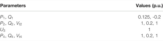
TABLE 3. Values of parameters.

Figure 12 demonstrates the overall trend of the voltage and the current when loads decrease with an increased load impedance in the improved APME model. The amplitude of current change is larger than that of voltage, and the changes of voltage and current amplitudes of L2 are larger than those of L1. The amplitude of current change is larger than that of voltage when the power of loads changes. It means that this model tries to keep the voltage stable. Obviously, when keeping the parameters of generator unchanged, the increase of the loads causes the reallocation of the power of the power system, and the voltage at the load bus will decrease, which is consistent with the actual operation situation.

FIGURE 12

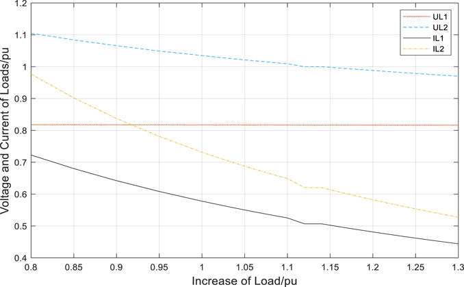
FIGURE 12. Voltage and current curves on load with the increase of load of the improved APME model.

The increased load in a typical APME model is studied too (shown in Figure 13). The changes and trends of the voltage and the current are the same with the improved model proposed in this paper. Table 4 shows the voltage and current of L2 before and after being improved in the DFIG model, in the same scenario of the increased load, which once again proves the following conclusion: this model keeps the voltage stable, and both the improved and typical models have the same dynamic trends when loads increase.

FIGURE 13

FIGURE 13. Voltage and current curves on load with the increase of load of the typical APME model.

TABLE 4

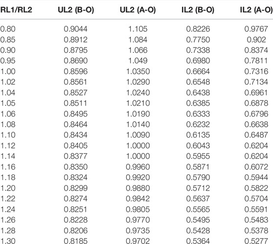
TABLE 4. Voltage and current details of Load 2 before and after improvement (per unit).

5 Conclusion

An improved APME model for transient analysis based on the amplitude–phase motion equation has been proposed in this paper. In the actual transient process, the decrease of voltage amplitude or the flicker of voltage phase will affect the phase dynamics of DFIG. Based on the typical amplitude–phase motion equation model of DFIG, the phase dynamics of DFIG is improved, and a different expression of ${\theta }_{err}$ is derived, which is equivalent to adding a feedback control to the control loops of DFIG. The amplitude of the terminal voltage and the q-axis current are introduced to influence the phase error of the PLL. That is, the output current of the current control unit and the terminal voltage amplitude are introduced into the phase control loop of the terminal voltage, so that the phase output of the terminal voltage can directly reflect the terminal voltage amplitude. As a result, the control loop inside the DFIG is improved, and the coupling model becomes stronger, which makes the operation characteristics closer to the real scenarios. When the wind speed changes sharply, the proposed model in this paper has better robustness and smooth operation ability than the typical one.

Data Availability Statement

The original contributions presented in the study are included in the article/Supplementary Material, and further inquiries can be directed to the corresponding author.

Author Contributions

QL was responsible for modeling and writing. MC was responsible for the simulation. YJ was responsible for reviewing and modification. DZ and RZ were responsible for data calculation. SC and CZ were responsible for feasibility verification.

Funding

This study was supported by the NSFC under Grant No. 51677020.

Conflict of Interest

The authors declare that the research was conducted in the absence of any commercial or financial relationships that could be construed as a potential conflict of interest.

Publisher’s Note

All claims expressed in this article are solely those of the authors and do not necessarily represent those of their affiliated organizations, or those of the publisher, the editors, and the reviewers. Any product that may be evaluated in this article, or claim that may be made by its manufacturer, is not guaranteed or endorsed by the publisher.

References

Arabi, S., Kundur, P., Hassink, P., and Matthews, D. (2000). “Small Signal Stability of a Large Power System as Affected by New Generation Additions[C],” in 2000 Power Engineering Society. Summer Meeting (Cat. No.00CH37134), 16-20 July 2000, Seattle, WA, USA (IEEE), 2, 812–816.

Google Scholar

Clark, K., Miller, N., and Sanchez-Gasca, J. (2010). Modeling of GE Wind Turbine-Generators for Grid Studies(version 4.5) [R]. New York: General Electric International,Inc.

Google Scholar

Duan, Q., and Sheng, W. (2019). Stability Analysis of Power Routers Connected to Power Electronic Distribution Grid[J]. Power Syst. Technol. 43 (01), 227–235. doi:10.13335/j.1000-3673.pst.2018.0753

CrossRef Full Text | Google Scholar

Ebrahimzadeh, E., Blaabjerg, F., Wang, X., and Bak, C. L. (2019). Optimum Design of Power Converter Current Controllers in Large-Scale Power Electronics Based Power Systems. IEEE Trans. Ind. Applicat. 55 (3), 2792–2799. doi:10.1109/tia.2018.2886190

CrossRef Full Text | Google Scholar

Gao, J., Zhao, J., Qu, K., and Li, F. (2018). “Reconstruction of Impedance-Based Stability Criterion in Weak Grid[J],” in 2018 3rd International Conference on Intelligent Green Building and Smart Grid (IGBSG), Yilan, Taiwan, 22-25 April 2018 (IEEE), 1–4. doi:10.1109/IGBSG.2018.8393572

CrossRef Full Text | Google Scholar

He, M., He, W., Hu, J., Yuan, X., and Zhan, M. (2019). Nonlinear Analysis of a Simple Amplitude-phase Motion Equation for Power-Electronics-Based Power System. Nonlinear Dyn. 95 (3), 1965–1976. doi:10.1007/s11071-018-4671-6

CrossRef Full Text | Google Scholar

Huang, H., Ju, P., Pan, X., Jin, Y., Yuan, X., and Gao, Y. (2019). Phase-amplitude Model for Doubly Fed Induction Generators. J. Mod. Power Syst. Clean. Energ. 7 (2), 369–379. doi:10.1007/s40565-018-0450-0

CrossRef Full Text | Google Scholar

Li, S., Yan, Y., and Yuan, X. (2019). SISO Equivalent of MIMO VSC-Dominated Power Systems for Voltage Amplitude and Phase Dynamic Analyses in Current Control Timescale. IEEE Trans. Energ. Convers. 34 (3), 1454–1465. doi:10.1109/tec.2019.2908222

CrossRef Full Text | Google Scholar

Liu, J., Miura, Y., Bevrani, H., and Ise, T. (2021). A Unified Modeling Method of Virtual Synchronous Generator for Multi-Operation-Mode Analyses[J]. IEEE J. Emerging Selected Top. Power Elect. 9 (2), 2394–2409. doi:10.1109/JESTPE.2020.2970025

CrossRef Full Text | Google Scholar

Sun, J. (2011). Impedance-Based Stability Criterion for Grid-Connected Inverters. IEEE Trans. Power Electron. 26 (11), 3075–3078. doi:10.1109/tpel.2011.2136439

CrossRef Full Text | Google Scholar

Wang, X., and Blaabjerg, F. (2019). Harmonic Stability in Power Electronic-Based Power Systems: Concept, Modeling, and Analysis. IEEE Trans. Smart Grid 10 (3), 2858–2870. doi:10.1109/tsg.2018.2812712

CrossRef Full Text | Google Scholar

Wen, B., Boroyevich, D., Burgos, R., Mattavelli, P., and Shen, Z. (2016). Analysis of D-Q Small-Signal Impedance of Grid-Tied Inverters. IEEE Trans. Power Electron. 31 (1), 675–687. doi:10.1109/tpel.2015.2398192

CrossRef Full Text | Google Scholar

Wu, T., Xie, X., and Jiang, Q. (2021). Three-port Admittance Modeling of Grid-Connected Converters Considering Frequency-Coupling and AC/DC Coupling Effects[J]. Proc. CSEE 42 (1), 248–259. doi:10.13334/j.0258-8013.pcsee.210330

CrossRef Full Text | Google Scholar

Yan, X., Cui, S., Sun, X., and Sun, Y. (2021). Transient Modeling of Doubly-Fed Induction Generator Based Wind Turbine on Full Operation and Rapid Starting Condition[J]. Power Syst. Technol. 45 (04), 1250–1260. doi:10.1049/rpg2.12090

CrossRef Full Text | Google Scholar

Yan, Y., Yuan, X., and Hu, J. (2016). “Interaction Analysis of Multi VSCs Integrated into Weak Grid in Current Control time-Scale[C],” in 2016 IEEE Power an. Energy Society General Meeting (PESGM), Boston, MA, USA, 17-21 July 2016 (IEEE), 1–6. doi:10.1109/PESGM.2016.7741677

CrossRef Full Text | Google Scholar

Yang, Z., Mei, C., Cheng, S., and Zhan, M. (2020). Comparison of Impedance Model and Amplitude-phase Model for Power- Electronics-Based Power System. IEEE J. Emerg. Sel. Top. Power Electron. 8 (3), 2546–2558. doi:10.1109/jestpe.2019.2927109

CrossRef Full Text | Google Scholar

Yuan, H., and Yuan, X. (2018). Modeling and Characteristic Analysis of Grid-Connected VSCs Based on Amplitude-phase Motion Equation Method for Power System Transient Process Study in DC-Link Voltage Control Timescale[J]. Proc. CSEE 38 (23), 6882–6892+7122. doi:10.13334/j.0258-8013.pcsee.180103

CrossRef Full Text | Google Scholar

Yuan, X., Cheng, S., and Hu, J. (2016). Multi-time Scale Voltage and Power Angle Dynamics inPower Electronics Dominated Large Power Systems[J]. Proc. CSEE 36 (19), 5145–5154+5395. doi:10.13334/j.0258-8013.pcsee.161247

CrossRef Full Text | Google Scholar

Yuan, X., Hu, J., and Cheng, S. (2017). Multi-time Scale Dynamics in Power Electronics-Dominated Power Systems. Front. Mech. Eng. 12 (3), 303–311. doi:10.1007/s11465-017-0428-z

CrossRef Full Text | Google Scholar

Zhang, D., Ying, J., and Yuan, X. (2017). Modelling and Optimization of Wind Turbine Electromechanical Transient Characteristics Using Magnitude Phase Motion Equation[J]. Proc. CSEE 37 (14), 4044–4051+4283. doi:10.13334/j.0258-8013.pcsee.170597

CrossRef Full Text | Google Scholar

Zhang, M., Yuan, X., and Hu, J. (2018). Inertia and Primary Frequency Provisions of PLL-Synchronized VSC HVDC when Attached to Islanded AC System. IEEE Trans. Power Syst. 33 (4), 4179–4188. doi:10.1109/tpwrs.2017.2780104

CrossRef Full Text | Google Scholar

Zhao, M., Yuan, X., and Hu, J. (2018). Modeling of DFIG Wind Turbine Based on Internal Voltage Motion Equation in Power Systems Phase-Amplitude Dynamics Analysis. IEEE Trans. Power Syst. 33 (2), 1484–1495. doi:10.1109/tpwrs.2017.2728598

CrossRef Full Text | Google Scholar

Zong, H., Zhang, C., Lyu, J., Cai, X., Molinas, M., and Rao, F. (2020). Generalized MIMO Sequence Impedance Modeling and Stability Analysis of MMC-HVDC with Wind Farm Considering Frequency Couplings. IEEE Access 8, 55602–55618. doi:10.1109/access.2020.2981177

CrossRef Full Text | Google Scholar