 Xianbao Yuan1,2
 Jingyu Wei1,2*Binhang Zhang1,2Yuefeng Guo1,2Qiang Shi1,2Pan Guo1,2Senquan Yang3Chao Tan3
- 1College of Mechanical and Power Engineering, China Three Gorges University, Yichang, China
- 2Hubei Key Laboratory of Hydroelectric Machinery Design and Maintenance, China Three Gorges University, Yichang, China
- 3China Nuclear Power Operation Technology Corporation, Ltd., Wuhan, China
Radioactive aerosol will transport in the containment and also will leak into the environment under a severe nuclear accident. Thus, it is of great significance for predicting the behavior of aerosol under a severe nuclear accident. In order to analyze the aerosol behavior, an improved multi-component sectional model is developed, which improves section numbers and updates the aerosol particle density at each time step. The model’s dependability is confirmed to use benchmark and experimental values. An excellent agreement can be observed between simulation and benchmark. On this premise, the LBLOCA accident is chosen to explore the behavior of radioactive aerosol in the containment. The finding shows that the aerosol is mostly deposited on the structure’s surface due to gravity in the LBLOCA accident. According to a comparison of the influence of aerosol natural deposition mechanisms on the distribution of diameter particles, Brownian diffusion, thermophoresis, diffusiophoresis, and gravity all have an effect on aerosol in the range of 0.01
Introduction
After the Fukushima accident, the study of severe accidents (SA) has gained more international attention (Wittneben, 2012). In a hypothetical nuclear power plant severe accident, the release of radioactive fission products can occur from the core fuel, the fuel-cladding gap, and the material in the cavity. The fission product released by core melting will leak into the containment through the primary system break, and if the accident deteriorates further, it will lead to containment failure, resulting in radioactive fission products being released into the environment (Allelein et al., 2009; Lin, W. et al., 2014). Radioactive fission products exist as gases, aerosols, or deposited onto heat structure, and the most radioactive fission products within the containment are transported with the movement of the aerosol (Soffer et al., 1995). Aerosol particles released into the containment will change due to collisions between particles, and some of the aerosol particles will deposit onto the containment heat structure because of temperature, density, diffusion, and gravity (Raj Sehgal, 2012). Otherwise, the detailed aerosol property is necessary to calculate the radioactive aerosol removal efficiency of engineered safeguards, such as the spray system and the filtration system (Porcheron et al., 2008; Rýdl et al., 2019; Wang et al., 2021). Therefore, it is significant to study the radioactive aerosol distribution and the radioactive aerosol behavior under a severe nuclear accident.
In the past research studies, many researchers have developed codes to study the behavior of the radioactive aerosol. For instance, Klinik et al. (2010) used the integrated program ASTEC to perform transient simulations of thermal-hydraulic phenomena and aerosol behavior in tests on containment systems of different sizes, such as the Phebus. The FP containment bench, the KAEVER containment bench, and the Battelle containment bench obtained good simulation results. For the deposition and coagulation behavior of aerosols in a nuclear reactor, Alipchenkov et al. (2009) have developed a code for calculating the behavior of aerosol-shaped fission products in the primary circuit of a nuclear reactor, which focuses on the development of models for predicting the deposition and coagulation rate of aerosols. There are also many numerical studies to solve the aerosol general dynamic equation, such as the sectional method (Gelbard and Seinfeld, 1980), the moment method (Wang et al., 2019), the discrete-sectional method (Li and Cai, 2020), and the Monte Carlo method (Bird, 1994; Liu and Chan, 2018). The sectional method is commonly used to describe the multicomponent aerosol dynamic behavior in the nuclear power plant. Because the sectional method requires the number of sections and the boundary of the section is fixed, this model also is called the fixed section model. MAEROS code developed based on the sectional method is widely used in the accident analysis program (Gelbard, 1982), such as MELCOR (Humphries et al., 2017) and CONTAIN (Murata et al., 1997). MAEROS is a multi-sectional, multi-component aerosol dynamic code that evaluates the size distribution of each type of aerosol mass, or component, as a function of time. MAEROS code also will deal with deposition processes of the radioactive aerosol. In the MAEROS code, the radioactive aerosol particles are allocated into fixed sections by particle volume, and the composition of the aerosol particles in the same section is considered uniform.
This sectional method discussed previously has fixed a section boundary and constant section number, and the aerosol particle density is constant by the input data. As known, when the reactor core begins melting in a severe accident, the radioactive aerosol source will continuously change along with the development of the accident, and the radioactive aerosol components released from the reactor core are also different. Moreover, the radioactive aerosol coagulation behavior and deposition behavior will change the components of radioactive aerosol. Thus, the radioactive aerosol density is closely associated with the deposition behavior and coagulation behavior. In the MAEROS code, in order to simplify the coefficients, it restricts the maximum section number. The geometric constraint is
The objective of this research first proposes an improved multi-component sectional method to simulate aerosols under severe accident. Then, the improved model is verified and validated by the benchmark and experiment. Furthermore, this research investigates the distribution of CsI aerosol under the LBLOCA accident and the effect of the natural deposition mechanism and aerosol density on the aerosol distribution.
Mathematical Method
Aerosol Dynamic Models
The spatial and chemical composition of the particles are represented by the size distribution function
where
By discretizing the aerosol particles into
where
where
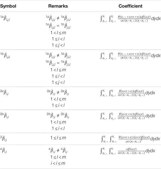
TABLE 1. Coagulation coefficients (Gelbard and Seinfeld, 1980).
Moreover, the first and second terms in the right of Eq. 3 indicate the flux of the radioactive aerosol component
Aerosol Removal Models
For the calculation of the deposition term in this study, gravity, Brownian diffusion, thermophoresis, and diffusiophoresis are considered for each heat structure surface of the containment, and the removal rate of all heat structure surfaces is added up to the total removal rate (Murata et al., 1997; Humphries et al., 2017).
where
where
Gravitational Deposition
where
The Cunningham slip correction factor in Eq. 6 is expressed as follows.
Here,
The gravitational deposition is effective for upward surfaces, such as the floor and pool. As for the downward surface, this mechanism will not act on it. Also, one basic hypothetical condition of this model is that the aerosol particle Reynolds number must be less than 1, which means that inertial effects of the flow may be neglected.
Brownian Diffusion
Brownian diffusion of aerosols refers to the deposition of aerosols due to mutual collision between the aerosol and the heat structure surface. The deposition velocity because of Brownian diffusion is defined as follows.
where
Thermophoresis
Thermophoresis is caused by the temperature gradient between the aerosol particles and heat structure surface, and the aerosol particles will deposit on the object surface at a lower temperature. The thermophoretic deposition velocity is defined as follows.
where
Diffusiophoresis
The diffusiophoresis process is also as known as a vapor condensation process. When the vapor condenses on the surface of the heat structure surface, composition gradients will exist in the adjacent gas, which will affect aerosol deposition behavior on the surface. The aerosol particles will remove along with the concentration gradient, which is caused by vapor condensation on the heat structure surface.
where
Improvement of the Multi-Component Sectional Method
The agglomeration kernels of the four mechanisms are proposed in the study by Humphries et al. (2017).
where
where
where
According to the traditional section method, if the coagulation coefficient is resolved at each time step, it will waste the computation time. Therefore, it is necessary to simplify the calculation process of the coagulation coefficient.
Such as
where the subscript
where the superscript ∗ represents the standard agglomeration coefficients and density. By analogy, the gravitational agglomeration can be written as
The turbulent agglomeration can be written as
According to the above equation, the standard agglomeration coefficients are only calculated before the iterative process. The coefficients of
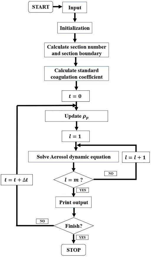
FIGURE 1. Flow chart of the model.
Verification and Validation of the Model
The aerosol model is validated by comparison with the benchmark, including two different coagulation problems and two different coagulation problems combined with deposition problems (Shaker et al., 2012). The aerosol model next is verified with the STORM experiment (Castelo et al., 1999), in which the main objective is to ensure the aerosol behaviors.
Validation With the Benchmark
Benchmark 1: Constant coagulation rate [
It is assumed that the coagulation rate is constant, and the deposition rate and source term are zero. The exact solution is as follows.
where
Benchmark 2: Linear coagulation rate [
Benchmark 3: Constant coagulation rate and a constant deposition rata [
Benchmark 4: Linear coagulation rate and a constant deposition rata [
The error value for the radioactive aerosol number of different section numbers between numerical and exact solutions to the equation GED is less than 10−3, as shown in Figure 2. The number of sections is selected as 20, 50, 100, and 300. The initial number of the radioactive aerosol number is 1 × 10¹⁰. By calculating the error value for chosen sections, the errors in the four selected sections gradually decreased. The error value is the least one when dividing the radioactive aerosol particle into 300 sections, as shown in Figure 2. It is mainly due to the effective reduction of the assumed initial distribution function when the number of sections increases. Therefore, the appropriate number of sections can be selected in the numerical simulation to reduce the error between the simulation values and the exact solution.
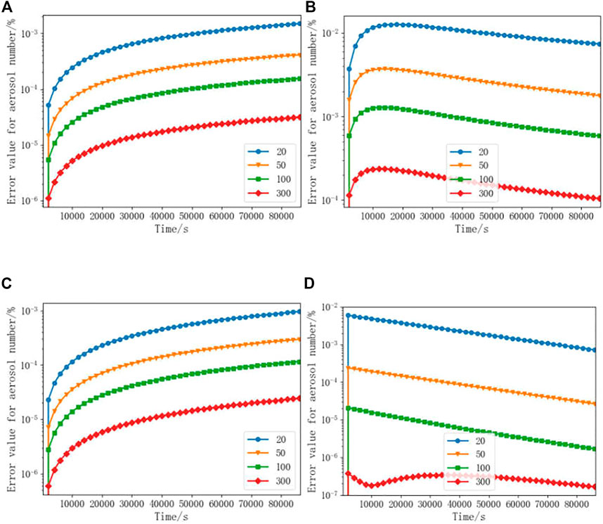
FIGURE 2. Error value for the number of radioactive aerosols for the different sections. [(A), Constant coagulation kernel; (B), linear coagulation kernel; (C), constant coagulation kernel and the constant deposition rate of particles; and (D), linear coagulation kernel and the constant deposition rate of particles].
The error value for the radioactive aerosol number of different initial particles between the numerical and exact solutions to the equation GDE is less than 10−3, as shown in Figure 3. The initial radioactive aerosol particle concentration is selected as
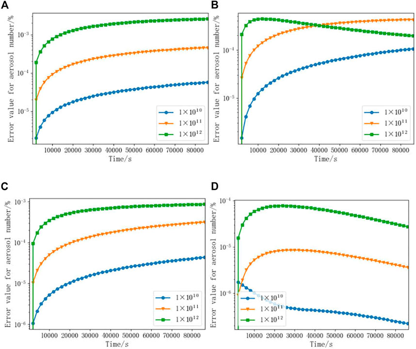
FIGURE 3. Error value for the number of radioactive aerosols for different initial particle numbers. [(A), Constant coagulation kernel; (B), linear coagulation kernel; (C), constant coagulation kernel and the constant deposition rate of particles; (D), linear coagulation kernel and the constant deposition rate of particles].
The distribution of the radioactive aerosol particle number is presented in Figure 4. The initial radioactive aerosol particle number is
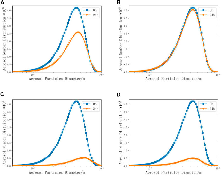
FIGURE 4. Distribution of radioactive aerosol particles. [(A), constant coagulation kernel; (B), linear coagulation kernel; (C), constant coagulation kernel and the constant deposition rate of particles; (D), linear coagulation kernel and the constant deposition rate of particles].
Verification With the Experiment
The STORM-SR11 test from the International Standard Problem 40 (ISP-40) is selected for aerosol model validation. The experiment consisted of two phases: the first focusing on deposition due to natural deposition mechanisms and the second on the resuspension process of aerosols under conditions of increased airflow. This study focuses on the first phase for validation.
Figure 5 shows a schematic diagram of the STORM test facility. The test section is a 5.0055 m long straight tube with an internal diameter of 63 mm made of stainless steel. In the deposition test, the supplied carrier gas and aerosol are mixed in a mixing tank and flow into the test section, where the exhaust from the test section is connected to a cleaning and filtration system. The aerosol used is tin oxide (SnO2), and the carrier gas is a mixture of nitrogen, steam, argon, helium, and air.
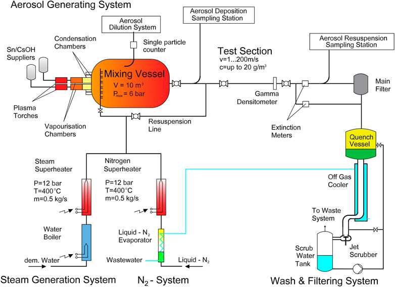
FIGURE 5. STORM experimental facility (Castelo et al., 1999).
The constant mass flow rate of the aerosol in the test is 3.83 × 10⁻⁴ kg/s. Assuming that its initial distribution follows a log-normal distribution, the number distribution particle size f(d) is defined as follows.
where
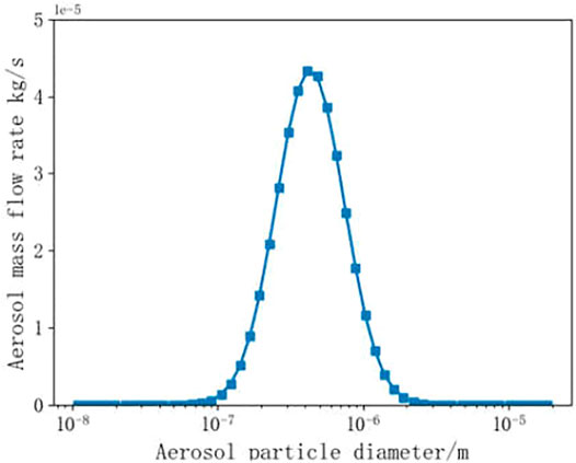
FIGURE 6. Initial aerosol distribution.
The time of the numerical simulation is the same as the experiment time of 9,000 s. Figure 7 shows the comparison between the simulated results and the experiment values. There are three distinct peaks, which are located at 1.02, 3.27, and 4.36 m. The maximum measured peak value is 0.292 kg/m2. The peak of the measured values in the experiment is caused by the uneven surface of the test pipe joints. The simulated results and the measured values of the smooth pipes agree very well, and they all show a constant decrease in the aerosol mass along the pipe. Table 2 depicts the deposition mass of the simulated and measured values. The deposition mass changes with the number of nodes. As the number of nodes increases, the error between the simulated value and the measured value also decreases, which gave the minimum error 6.19%.
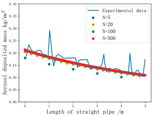
FIGURE 7. Aerosol deposition along with the test pipe.
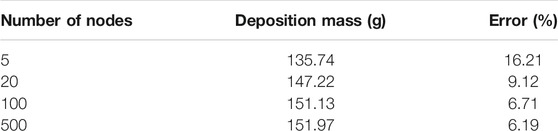
TABLE 2. The deposited mass.
Application of the Aerosol Model Under Severe Accident
Accident Sequences
In this research, an LBLOCA accident is selected to study the particle distribution and behavior of aerosols, with a breach diameter of 50 cm and a breach location in the hot leg. To maximize the release rate of aerosols under accident conditions, all safe injection systems in the primary system are shut down. The sequence of events is shown in Table 3, the pressure vessel failing at 5,489 s.
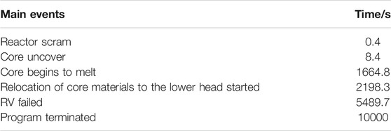
TABLE 3. Sequence of events.
According to the source term evaluation results after the Fukushima accident, when a serious accident occurs, the monitoring data for I131, Cs134, and Cs137 are the most nuclides, and they are also the widely important nuclides in the radiation evaluation. The air source term of I131 is 60–390 PBq, the air source term of Cs134 is 15–20 PBq, and the air source term of Cs137 is 5–50 PBq, after the accident (Bois et al., 2014; Cervone and Franzese, 2014; Koo et al., 2014). Therefore, this study focuses on the fission product CsI. Figure 8 shows the variation of the mass of CsI aerosols with time for the accident sequence. The aerosol starts to increase at 8 s due to core exposure; when the temperature exceeds the melting temperature at 1,664 s, the core starts to melt and the aerosol release rate starts to increase dramatically and reaches a peak, with a small increase at 5,489 s due to pressure vessel failure.
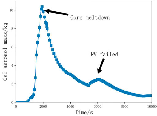
FIGURE 8. Change of the CsI aerosol mass with time.
As the accident proceeds, the aerosol mass will peak at 2,000 and 6,710 s. Figure 9 shows the distribution of the aerosol mass at 2,000, 6,710, and 10,000 s. According to the mass distribution, the CsI aerosol particles mainly concentrated at 0.41 um. The mass of the CsI aerosol mass at 2,000 s is maximum in the containment, as shown in Figure 8, and the max aerosol mass in Figure 9 is 2 kg. When the pressure vessel failure is at 5,489 s, the CsI aerosol mass rises again and reaches a maximum at 6,710 s, in which the max aerosol particle mass is 1.43 kg. At the end of the calculation, the CsI aerosol mass drops to 1.22 kg. It can also be seen that according to Figure 9, the distribution of the CsI aerosol mass is declining with the accident process.
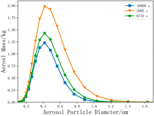
FIGURE 9. Distribution of the CsI aerosol mass.
Effect of the Natural Deposition on Aerosols
The natural deposition is the primary removal mechanism of aerosols. Thus, the effect of different natural deposition on aerosols is important. As shown in Figure 10, at the end of the simulation, gravity accounts for 54% of the total deposition mass, thermophoresis 28%, diffusion 3%, and Brownian diffusion 15%. Comparing the natural deposition mass of aerosols under the accident conditions, gravitational effect is more than the other three deposition mechanisms.
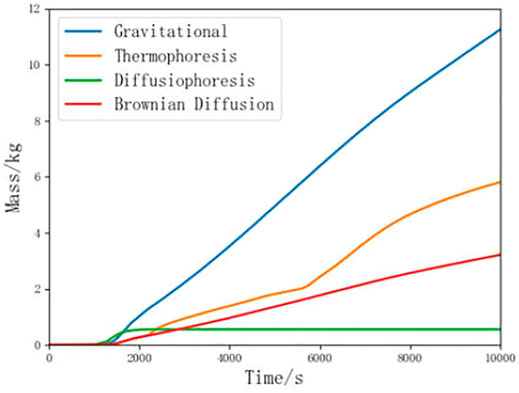
FIGURE 10. Natural deposition of the CsI aerosol within the containment.
Different deposition mechanisms can also have an impact on aerosol particle distribution. Figure 11 shows the effect of the different mechanisms on the aerosol particle. As can be seen from the figure, the natural deposition mechanism has a certain impact on the particles between 0.01
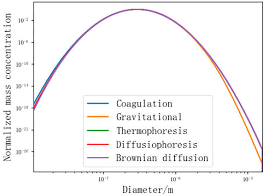
FIGURE 11. Effect of the deposition mechanism on the distribution of aerosol diameter particles.
Influence of the Aerosol Particle Density
In this section, the influence of the radioactive aerosol particle density of a seven-component problem is discussed. The detailed density of the seven components is listed in Table 4. The initial components’ mass concentration and the initial radioactive aerosol particle numbers are shown in Figure 12. The different line types represent different component mass distribution and the radioactive aerosol particle number distribution. CsI is defined as component 1, UO2 as component 2, H2O as component 3, Te as component 4, B2O3 as component 5, Cd as component 6, and Pb as component 7. Number distribution is the axis on the left. Other curves are the axis on the right.
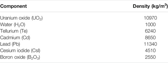
TABLE 4. Component densities.
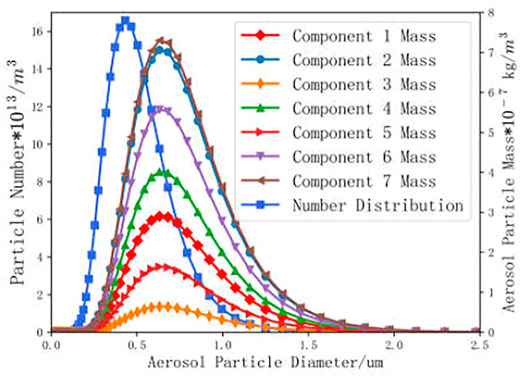
FIGURE 12. Initial aerosol distribution.
The particle number and component mass distribution in the presence of the aerosol coagulation process have been tabulated in Figures 13, 14. The difference in the radioactive aerosol particle number distribution can be seen in Figure 13. The aerosol particle number of the fixed density peaks at 0.45
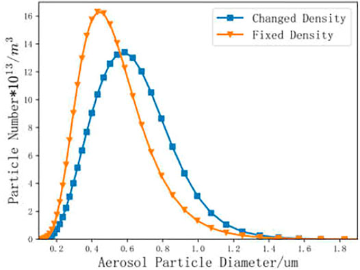
FIGURE 13. Effect of different densities on the aerosol particle number distribution.
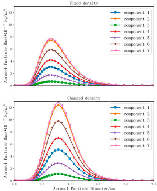
FIGURE 14. Effect of different densities on the component mass distribution.
Conclusion
This research adopts the improved multi-component aerosol sectional model to analyze the behavior of radioactive aerosol under severe accidents, which considers coagulation, deposition, and source term. The development model has demonstrated encouraging accuracy throughout the validation with the benchmark and experiment. The simulation result has a good agreement with the benchmark, where the error is less than 10−3. The comparison with the STORM experiment also has a satisfied result. The sensitivity analysis of the section number shows that the appropriate number can effectively improve the simulation error.
Furthermore, according to the analysis under the LBLOCA accident, gravity deposition is the main deposition method in the aerosol deposition mechanism, accounting for 54% of the total deposition. The natural deposition mechanism affects the particles in the 0.01
Data Availability Statement
The original contributions presented in the study are included in the article/Supplementary Material, further inquiries can be directed to the corresponding author.
Author Contributions
JW conceived and planned this work, wrote, and finalized the manuscript. XY and BZ provided constructive discussions. YG, QS, PG, SY, and CT contributed to review and revision.
Funding
This study is financially supported by the National Natural Science Foundation of China (Grant Nos. 12175116 and 11805112).
Conflict of Interest
Authors SY and CT were employed by the China Nuclear Power Operation Technology Corporation, Ltd.
The remaining authors declare that the research was conducted in the absence of any commercial or financial relationships that could be construed as a potential conflict of interest.
Publisher’s Note
All claims expressed in this article are solely those of the authors and do not necessarily represent those of their affiliated organizations, or those of the publisher, the editors, and the reviewers. Any product that may be evaluated in this article, or claim that may be made by its manufacturer, is not guaranteed or endorsed by the publisher.
References
Alipchenkov, V. M., Kiselev, A. E., Strizhov, V. F., Tsaun, S. V., and Zaichik, L. I. (2009). Advancement of Modeling Deposition and Coagulation of Aerosols in a Nuclear Reactor. Nucl. Eng. Des. 239 (4), 641–647. doi:10.1016/j.nucengdes.2008.12.025
Allelein, H. J., Auvinen, A., Ball, J. S. G., and Weber, G. (2009). State of the Art Report on Nuclear Aerosols. OECD Report NEA/CSNI/R(2009)5.
Bailly du Bois, P., Garreau, P., Laguionie, P., and Korsakissok, I. (2014). Comparison between Modelling and Measurement of marine Dispersion, Environmental Half-Time and 137cs Inventories after the Fukushima Daiichi Accident. Ocean Dyn. 64 (3), 361–383. doi:10.1007/s10236-013-0682-5
Bird, G. A. (1994). Molecular Gas Dynamics and the Direct Simulation of Gas Flows. Oxford Engineering Science Series. Oxford, New York: Clarendon Press, Oxford University Press.
Castelo, A. R., Capitao, J. A., and Santi, G. D. (1999). International Standard Problem 40 Aerosol Deposition and Resuspension. Magn. Reson. Med. 21 (2), 302–307.
Cervone, G., and Franzese, P. (2014). “Source Term Estimation for the 2011 Fukushima Nuclear Accident,” in Data Mining for Geoinformatics Methods and Applications. Editors G. Cervone, J. Lin, and N. Waters (New York: Springer), 49–64. doi:10.1007/978-1-4614-7669-6_3
Gelbard, F. (1982). MAEROS User Manual. Sandia National Laboratories Report SAND80-0822, U. S. Nuclear Regulatory Commission Report NUREG/CR-1391. doi:10.2172/6459120
Gelbard, F., and Seinfeld, J. H. (1978). Numerical Solution of the Dynamic Equation for Particulate Systems. J. Comput. Phys. 28 (3), 357–375. doi:10.1016/0021-9991(78)90058-X
Gelbard, F., and Seinfeld, J. H. (1980). Simulation of Multicomponent Aerosol Dynamics. J. Colloid Interf. Sci. 78 (2), 485–501. doi:10.1016/0021-9797(80)90587-1
Humphries, L. L., Beeny, B. A., Gelbard, F., Louie, D. L., and Phillips, J. (2017). MELCOR Computer Code Manuals. In Reference Manual (Vol. 2). Sandia National Laboratories Report SAND2017-0876 O. doi:10.2172/1433918
Kljenak, I., Dapper, M., Dienstbier, J., Herranz, L. E., Koch, M. K., and Fontanet, J. (2010). Thermal-hydraulic and Aerosol Containment Phenomena Modelling in ASTEC Severe Accident Computer Code. Nucl. Eng. Des. 240 (3), 656–667. doi:10.1016/j.nucengdes.2009.12.002
Koo, Y.-H., Yang, Y.-S., and Song, K.-W. (2014). Radioactivity Release from the Fukushima Accident and its Consequences: a Review. Prog. Nucl. Energ. 74 (3), 61–70. doi:10.1016/j.pnucene.2014.02.013
Li, C., and Cai, R. (2020). Tutorial: the Discrete-Sectional Method to Simulate an Evolving Aerosol. J. Aerosol Sci. 150, 105615. doi:10.1016/j.jaerosci.2020.105615
Lin, W., Chen, L., Yu, W., Ma, H., Zeng, Z., Lin, J., et al. (2014). Radioactivity Impacts of the Fukushima Nuclear Accident on the Atmosphere. Atmos. Environ. 102, 311–322. doi:10.1016/j.atmosenv.2014.11.047
Liu, H. M., and Chan, T. L. (2018). Two-component Aerosol Dynamic Simulation Using Differentially Weighted Operator Splitting Monte Carlo Method. Appl. Math. Model. 62 (OCT), 237–253. doi:10.1016/j.apm.2018.05.033
Murata, K. K., Williams, D. C., Tills, J., Griffith, R. O., Gido, R. G., Tadios, E. L., et al. (1997). Code Manual for Contain 2.0: A Computer Code for Nuclear Reactor Containment Analysis. Nuclear React. Tech.7. doi:10.2172/569132
Porcheron, E., Lemaitre, P., Nuboer, A., and Vendel, J. (2008). Heat, Mass and Aerosol Transfers in spray Conditions for Containment Application. Jpes 2 (2), 633–647. doi:10.1299/jpes.2.633
Rýdl, A., Fernandez-Moguel, L., and Lind, T. (2019). Modeling of Aerosol Fission Product Scrubbing in Experiments and in Integral Severe Accident Scenarios. Nucl. Tech. 205 (5), 655–670. doi:10.1080/00295450.2018.1511213
Shaker, M. O., Aziz, M., Ali, R., Sirwah, M., and Slama, M. (2012). Numerical and Analytical Solutions of the Aerosol Dynamic Equation in Reactor Containment. Arab J. Nucl. Sci. Appl. 45 (4), 96–108. http://www.esnsaeg.com/download/researchFiles/10_96-108.pdf.
Soffer, L., Burson, S. B., Ferrell, C. M., Lee, R. Y., and Ridgely, J. N. (1995). Accident Source Terms for Light-Water Nuclear Power Plants. Final Report. U.S. Nuclear Regulatory Commission. Washington, DC(United States): Division of Systems Technology. doi:10.2172/29438
Wang, F., Cheng, X., and Gupta, S. (2021). Cocosys Analysis on Aerosol Wash-Down of Thai-AW3 experiment and Generic Containment. Ann. Nucl. Energ. 153, 108076. doi:10.1016/j.anucene.2020.108076
Wang, K., Yu, S., and Peng, W. (2019). A Novel Moment Method Using the Log Skew normal Distribution for Particle Coagulation. J. Aerosol Sci. 134, 95–108. doi:10.1016/j.jaerosci.2019.04.013
Keywords: severe accident, radioactive aerosols, sectional model, LBLOCA, aerosol behavior
Citation: Yuan X, Wei J, Zhang B, Guo Y, Shi Q, Guo P, Yang S and Tan C (2022) Development and Application of an Aerosol Model Under a Severe Nuclear Accident. Front. Energy Res. 10:852501. doi: 10.3389/fenrg.2022.852501
Received: 11 January 2022; Accepted: 10 February 2022;
Published: 24 March 2022.
Edited by:
Yapei Zhang, Xi’an Jiaotong University, ChinaReviewed by:
Wei Peng, Tsinghua University, ChinaAlexandra Ioannidou, Aristotle University of Thessaloniki, Greece
Copyright © 2022 Yuan, Wei, Zhang, Guo, Shi, Guo, Yang and Tan. This is an open-access article distributed under the terms of the Creative Commons Attribution License (CC BY). The use, distribution or reproduction in other forums is permitted, provided the original author(s) and the copyright owner(s) are credited and that the original publication in this journal is cited, in accordance with accepted academic practice. No use, distribution or reproduction is permitted which does not comply with these terms.
*Correspondence: Jingyu Wei, bnVtYndqeUAxNjMuY29t