Spatial Electric Load Forecasting Method Based on High-Level Encoding of High-Resolution Remote Sensing Images

Spatial load forecasting (SLF) is important for regional power infrastructure construction planning and power grid management. However, for rapidly developing urban regions, SLF is generally inaccurate due to insufficient historical data. Hence, it is important to introduce the spatial load density (SLD) from similar regions to improve the accuracy of SLF. To select similar regions appropriately and acquire SLDs with limited available auxiliary data, this study proposes a spatial electric load forecasting method based on the high-level encoding of high-resolution remote sensing images called SELF-HE. In particular, SELF-HE introduces high-level ground object features as a key index to describe the characteristics of electric loads in a region and can establish connections between the remote sensing image features and SLD similarity. Based on this functionality, SELF-HE achieves more accurate SLF in regions with insufficient historical data. In the experiments, SELF-HE was compared with four traditional methods, and the results revealed that SELF-HE achieved improved SLF accuracy. Given that the high-resolution remote sensing images fully covered urban areas and were readily obtained, the proposed method can improve the accuracy of SLF with extremely low data collection costs and is applicable to rapidly developing urban regions.

Introduction

Efficient electric load forecasting methods can be employed to determine the electric load within a given period and provide considerable support for power grid management (Evangelopoulos et al., 2020; Moreno-Carbonell et al., 2020). Spatial load forecasting (SLF) indicates the extent to which the load will increase within a geographical region, which is necessary for determining the capacity or distribution of the equipment within a certain service zone (Willis and Tram, 1983; Willis, 2002). SLF can identify subzones with the highest anticipated load growth and support advanced preparations for distribution network expansion planning (Carreno et al., 2010; Melo et al., 2014; Han et al., 2020). Therefore, it is necessary to obtain high-quality SLF results.

To perform SLF, one of the following two conditions is required: 1) a long-term study based on multiple years of historical data to reflect the characteristics of load changes during various time periods during festivals and under different weather conditions, which requires a sufficiently long time series of data to construct a high-performance regression model (Georgilakis and Hatziargyriou, 2015; Xie et al., 2018), or 2) the ability to obtain directly the upcoming electric consumption plans of enterprises in the region and/or information pertaining to the regional economic growth or employment level to be used to assist in forecasting (Chow et al., 2005). The two above-mentioned conditions can be met in relatively stable and established urban areas. However, for rapidly developing cities, especially areas of new development, this information is difficult to obtain. Moreover, various regions were developed recently (especially within the past year), enabling the accumulation of sufficient time series data to develop regression models. Furthermore, electric consumption plans are difficult to obtain due to large changes in population or the unwillingness of companies to disclose their production plans (Wu and Lu, 2002; Salvó and Piacquadio, 2017).

With regard to the research on performing SLF via spatial load density (SLD), the implementation of SLF for areas of new development in cities for the analysis of the SLD is a feasible solution (He et al., 2015). For a newly developed plot p_x, if an existing plot p can be established with an electric load trend that is similar to that of p_x, the SLD of p can be obtained by normalizing the historical electric load data, which can be used in combination with the range of p_x to simulate a long time series of data to train a forecasting model. This strategy is effective for plots with insufficient historical load data (Yao et al., 2015; Ye et al., 2019). The advantage of using such SLD methods is the ability to identify “similar” plots. Given that a plot load is closely related to the objects/buildings on the ground, the optional source of information for determining “similar” plots is geospatial information.

Spatial feature information has a significant influence on the accuracy of SLF, and using a geographic information system (GIS) to describe and distinguish different SLD patterns is an effective means of obtaining spatial–temporal forecasting models (Monteiro et al., 2005; Brunoro et al., 2009; Shin et al., 2011). Based on the introduction of geospatial features, the SLF accuracies achieved with fuzzy clustering, spatial correlation, cellular automaton, and multiagent methods can all be effectively improved (Ying and Pan, 2008; Melo et al., 2010; Melo et al., 2012). However, most existing geographic information is not directly suitable for SLF or SLD processing, and this information is relatively neutral (Vasquez-Arnez et al., 2008). Therefore, most SLD-based methods adopt one of the following strategies: 1) the nearest plot is directly considered a similar source or 2) a plot in the same land use category is selected. For areas with a single industry and homogeneous structure, these two strategies are effective. However, for areas with highly diverse content, neighbor relationships or land use categories are not sufficient for identifying similar plots (Melo et al., 2015; Shi et al., 2016). For example, machinery manufacturing and biopharmaceutical companies belong to the economic development category (same land-use type); however, they exhibit completely different electricity consumption characteristics. Moreover, in areas of new urban development, this heterogeneity is severe (Ye et al., 2019). Therefore, it is necessary to study methods of achieving relatively accurate SLF with insufficient electric load time series data and approximate geographic information data.

For geographic information data to support SLF and SLD processing specifically, high-resolution remote sensing images constitute an appropriate source. With the advances in satellite sensor technology, high-resolution remote sensing images are becoming available, which can provide detailed ground object information (Pan et al., 2021). High-resolution remote sensing images can be used to obtain the structural and spatial details of the objects in urban areas rapidly and efficiently and provide decision-making support for critical information related to the status, planning, population, and environment of these areas (Li et al., 2016; Su et al., 2021; Plant et al., 2022). The specific characteristics of objects in a certain region can be extracted from remote sensing images (Srivastava et al., 2019; Chakraborty et al., 2021; Pristeri et al., 2021). At present, shallow models such as support vector machines (SVMs), decision trees, k-nearest neighbor (k-NN) models, and deep models, including convolutional neural networks (CNNs) and long short-term memory (LSTM) networks, can all be used to describe the characteristics of the contents of remote sensing images; adequate application results have been obtained in various fields (Yuan et al., 2017; Park et al., 2018; Li et al., 2019; Zhang et al., 2019; Kang et al., 2020). Similarly, the information required for SLF and SLD processing can be extracted from remote sensing images.

To address the difficulties in realizing SLF for rapidly developing regions, this study proposes a spatial electric load forecasting method based on the high-level encoding of high-resolution remote sensing images called SELF-HE. In SELF-HE, deep neural networks are established to obtain the features of ground objects from remote sensing images, an unsupervised clustering process is applied to establish connections between the image features and SLD, and a high-level encoding model is constructed to extract load characteristics from images. Using this model, data-rich plots that are similar to a given plot can be identified based on the features of the corresponding remote sensing images, enabling the use of the SLDs of similar plots to solve the problem of insufficient historical data. In the experiments, we tested the use of the proposed SELF-HE method for SLF in the northern part of Changchun, China. The results revealed that, compared with traditional methods, SELF-HE can achieve more accurate SLF. Moreover, SELF-HE uses only remotely sensed high-level feature data as the basis for identifying similar plots; hence, this method is beneficial for large-scale and low-cost SLF.

Methodology

Basic Principle of Using SLD for SLF

To achieve load forecasting for plots with insufficient historical electric load data, the proposed method applies the principle illustrated in Figure 1.

FIGURE 1

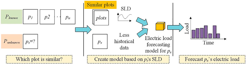
FIGURE 1. Basic principle of using SLD for SLF.

As shown in Figure 1, there are plots in a large zone Z: {p₁, p₂, … , p_n}. For each p_i = (area, history, sld), area is the spatial area corresponding to p_i, history is the time series data of the historical electric loads, and sld is the SLD vector calculated based on history. Elements in Z can be further separated into two types: P_known and P_unknown. The difference between P_known and P_unknown is that the elements of known originate from areas that were developed a sufficiently long time ago, where rich historical load data are available; by contrast, the elements of P_unknown correspond to newly developed urban areas, for which sufficient historical data have not been accumulated. Owing to the insufficiency of historical data, a sufficiently accurate forecasting model cannot be constructed. However, we can identify plots in P_known that are highly similar to those in P_unknown and use the SLDs of these plots to construct a forecasting model jointly based on the SLD information and a small amount of historical data.

Overall Process of the Proposed Method

The core problem in Figure 1 is to obtain the SLD information for a given plot p_x based on a set of plots similar to p_x in P_known. The spatial structure and style of buildings in high-resolution remote sensing images can provide information to solve this problem. Thus, we can use the high-level features of ground objects to perform an approximate search and obtain the target SLD. Hence, this study proposes the SELF-HE method. The overall process of SELF-HE is depicted in Figure 2.

FIGURE 2

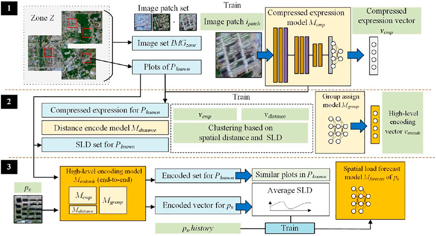
FIGURE 2. Overall process of SELF-HE.

As shown in Figure 2, for Zone Z containing plots belonging to known and unknown, the objective is to develop an SLF model for plot p_x in P_unknown. The SELF-HE consists of three steps:

Compressed Representation of Image Patches

Suppose that Z is depicted in one or more high-resolution remote sensing images IMG_zone = {img₁, img₂, … , img_n}. Based on the plots in P_known, the corresponding image patches are cut from IMG_zone to obtain the image patch set I_known = {i₁, i₂, … , i_n}. All data in I_known are then used to train a compressed representation model, namely, M_cmp. Using M_cmp, an image patch can be converted into a compressed representation vector, v_cmp. This step is described in detail in Compressed Representation of Image Patches.

Construction of a Distance Encoding Model and Group Assignment Model

Using M_cmp, I_known can be transformed into a set of compressed representation vectors. A distance encoding model M_distance is then constructed based on the locations of the plots. Using M_distance, each plot can be associated with a distance vector v_dis. Based on v_dis and SLD, the plots can be clustered, and the plots in P_known can be further encoded based on the clustering result T_cluster. Thereafter, a group assignment model M_group is constructed and trained based on v_dis, v_cmp, and T_cluster. The output of M_group is high-level encoding, which serves as the basis for SELF-HE to determine the degree of similarity between the plots. This step is described in detail in Construction of a Distance Encoding Model and Group Assignment Model.

High-Level Encoding and SLF

It should be noted that SELF-HE integrates M_distance, M_cmp, and M_group to construct a high-level encoding model, namely, M_encode. In particular, M_encode can realize an end-to-end plot encoding function, as it accepts the corresponding image patch and features of a plot as inputs and outputs the encoding result. For P_known, M_encode is used to obtain encoding result V_encode for each plot. For p_x, M_encode is used to obtain encoding result v_x. Thereafter, using the vector distances between v_x and the elements in V_encode, SELF-HE can identify P_similar plots in P_known that are the most similar to p_x. Based on P_similar and the historical data for p_x, an SLF model M_forecast for p_x can be obtained. This step is described in detail in High-Level Encoding and SLF.

Using the three steps above, although the plot corresponding to p_x is a newly established area in the city in which historical electric load data are scarce; based on the characteristics of the high-level encoding, an approximately similar area in the city can be identified, for which a large amount of historical data is available to facilitate the construction of M_forecast. Thereafter, M_forecast can be used to perform SLF for the area corresponding to p_x.

Compressed Representation of Image Patches

This section details the development of a compressed image patch representation model M_cmp, through which the high-level information in an image patch can be extracted. The structure of M_cmp is shown in Figure 3.

FIGURE 3

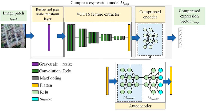
FIGURE 3. Structure of M_cmp.

As shown in Figure 3, M_cmp consists of three components:

Resize and Grayscale Transform Layer

As the first component of M_cmp, we introduce a layer that converts the input image into a grayscale image and then scales it to a specified size Param_size. The default value of Param_size is 256 × 256. There are two reasons for using this layer in M_cmp. First, with increasing resolution of a remote sensing image, the coverage area decreases; therefore, to cover all areas in Z, it may be necessary to use multiple images. In this case, even if these images are collected from the same satellite sensor, it is difficult to ensure that the images are consistent with respect to the acquisition time or season. To overcome this challenge, grayscale images can reduce the influence of vegetation growth on the color (certain band values) in an image, avoiding the case in which the subsequent neural network focuses on the color instead of the structure of the ground objects. Second, using a fixed output size in this layer can significantly reduce the difficulty of subsequent training. This layer can be realized using a color-to-grayscale conversion function [mapping the value range to (0, 1)] and an image resizing function, and the output is the feature map i_gray.

VGG16 Feature Extractor

The main objective of the second component of M_cmp is to extract high-level features from the input image. We directly use the pretrained VGG16 neural network to achieve this goal. This neural network contains five groups of feature extraction layers, each consisting of convolution + rectified linear unit (ReLU) and max pooling layers. One group of layers reduces the size of the input feature map by half. The pretrained VGG16 neural network does not require training. The standard pretrained weights obtained based on the ImageNet training samples are directly used as weights. At the end of the VGG16 network, we add a flattened layer to convert the output feature maps into one-dimensional vectors.

Vector v_flatten represents the representation result for the image patch. However, this vector comprises thousands of dimensions. With such high dimensionality, there is considerable redundant content that is not useful for distinguishing the differences between object structures in image patches, and an excessively high number of dimensions can readily cause overfitting in subsequent processing. Therefore, an additional compression process is required.

Compressed Encoder

In SELF-HE, an unsupervised approach is adopted to compress the output of the VGG16 feature extractor. First, we developed an autoencoder model. This model consists of an encoder M_encoder and a decoder M_decoder, which performs the following transformations:

$\{\begin{array}{c}\varphi :v_{flatten}\to encode\\ \phi :encode\to v_{flatten}\end{array}(1)$

The autoencoder model is expected to achieve the following via M_encoder and M_decoder:

$argmi{n}_{\varphi ,\phi }\Vert v_{flatten}-\left(\varphi \circ \phi \right)v_{flatten}\Vert (2)$

The encoder consists of three layers: a ReLU layer with a number of neurons equal to the dimensionality of v_flatten, a ReLU layer with 256 neurons, and a ReLU layer with Param_code neurons. Similarly, the decoder consists of three layers: a ReLU layer with Param_code neurons, a ReLU layer with 256 neurons, and a sigmoid layer with a number of neurons equal to the dimensionality of v_flatten. Using M_encoder, v_flatten is compressed into encoding with Param_code dimensions, whereas M_decoder attempts to restore encode to v_flatten. Using only M_encoder, v_flatten can be compressed into a Param_code-dimensional vector (default value of 32). Using M_encoder as the third component of M_cmp, the final output v_cmp can be obtained.

Based on the above description, the construction and training process for M_cmp is summarized in Algorithm 1.

Algorithm 1. M_cmp construction and training (MCP-CT) algorithm.

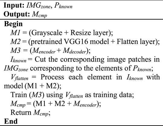
The MCP-CT algorithm accepts IMG_zone and P_known as the input and generates the M_cmp model after training. Moreover, M_cmp can compress and encode an image patch based on the differences with respect to all related images in known, and it outputs the compressed representation vector v_cmp.

Construction of a Distance Encoding Model and Group Assignment Model

This section details the determination of the distance encoding model M_distance and group assignment model M_group. Plots can then be encoded using these two models.

For Zone Z, suppose that the lower left corner is positioned at the two-dimensional coordinates (0, 0), the width of Z is L_width, and the height is L_height. The distances of a plot p_i from the coordinates (0, 0) along the x and y axes are denoted by p_i.area.x and p_i.area.y, respectively. Accordingly, the following equation is used to describe the relative position of p_i in Zone Z

$v_{distance}=\left(\frac{p_i.area.x}{L_{width}},\frac{p_i.area.y}{L_{height}},\frac{p_i.area.x}{L_{width}}-0.5,\frac{p_i.area.y}{L_{height}}-0.5\right),(3)$

where v_distance describes the position of p_i relative to the center of Z and relative to the coordinates (0, 0). For a plot, Eq. 3 can describe its position according to the distance from the starting point and the center point of Z, and form a vector; this vector is easy to participate in the calculation process of the neural network, v_distance can assist neural network take plot’s location as important features during inference. M_distance consists of a single layer with an input of p_i.area and output of v_distance; thus, M_distance can be used to realize end-to-end coding distance coding for a plot.

To develop M_group, we established the relationship between the SLD and the image encoding of a plot. This process is illustrated in Figure 4.

FIGURE 4

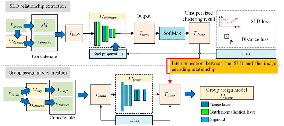
FIGURE 4. Process of establishing the relationship between the SLD and the image encoding of a plot.

As shown in Figure 4, the process of development and training consists of two steps.

SLD Relationship Extraction

For plot p_i, v_distance is first obtained using M_distance and is then concatenated with p_i.sld. Thereafter, the data from all plots in P_known are aggregated into an input sample batch T_batch. For SELF-HE, a deep neural network M_sldcluster is then used to cluster all samples in T_batch. M_sldcluster contains three groups of layers, each consisting of a dense layer and a batch normalization layer. The output of the final dense layer is N_category (default value is 64). Moreover, M_sldcluster encodes all samples in T_batch, and the encoding result is T_norm, which consists of nondimensional vectors. It should be noted that T_norm can be regarded as a fuzzy representation of the clustering of the samples; by applying ArgMax, the final clustering result T_cluster can be obtained. The difference between T_cluster and T_norm can be used as a loss function for training M_sldcluster:

$loss\left(T_{norm},T_{cluster}\right)=los{s}_{sld}\left(T_{norm},T_{cluster}\right)+los{s}_{distance}\left(T_{norm}\right).(4)$

Here, loss_sld represents the loss of the output in terms of the SLD difference, which can be expressed as follows:

$los{s}_{sld}\left(T_{norm},T_{cluster}\right)={\displaystyle \sum }_{i=1}^{N_{samples}}{\displaystyle \sum }_{j=1}^{N_{category}}\left(-\delta \left(j-T_{cluster}\left[i\right]\right)ln\left(T_{norm}\left[i\right]\left[j\right]\right)\right),(5)$

where $\delta \left(t\right)=\{\begin{array}{c}1 t=0\\ 0 t\ne 0\end{array}$. In addition, loss_distance represents the spatial neighboring constraint and is defined as

$los{s}_{space}\left(T_{norm}\right)={\displaystyle \sum }_{i=1}^{N_{samples}}\Vert T_{norm}\left[j\right]-T_{norm}\left[neighbor\left(j\right)\right]\Vert ,(6)$

where neighbor(j) denotes the number corresponding to the element nearest to Sample j. Eq. 4 considers constraints on the SLD similarity and spatial continuity. Accordingly, plots with close distances and similar SLDs are assigned to the same cluster. Moreover, M_sldcluster undergoes iterative backpropagation to improve the clustering results, as expressed by Algorithm 2.

Algorithm 2. SLD relationship extraction (SLD-E) algorithm.

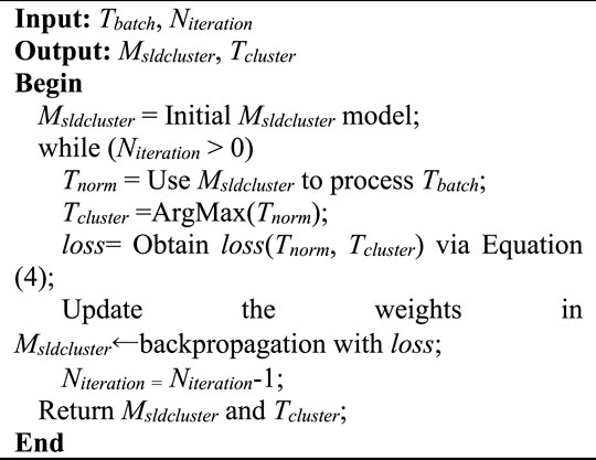
Using SLD-E, the clustering results T_cluster for all plots in P_known can be obtained. Plots with close spatial distances and relatively similar SLDs are mapped to the same category. Moreover, T_cluster captures the relationship between the SLD in space and the electric load trend. This relationship serves as a basis for the establishment of the relationship between image encoding and SLD similarity.

Group Assignment Model Creation

As shown in Figure 4, after T_cluster is obtained in Step 1, the group assignment model M_group can be trained. M_group consists of five dense layers and one sigmoid layer. For the elements in P_known, M_cmp is used to obtain the compressed image encoding v_cmp, M_distance is used to obtain v_distance, and v_cmp and v_distance are concatenated. In this manner, a description T_trainx corresponding to the image content and location information in P_known is generated. Moreover, T_cluster is used as the model output T_trainy. Thereafter, M_group is trained using T_trainx and T_trainy. By training M_group, the relationship between image encoding and SLD clustering results is established. This process is expressed by Algorithm 3.

Algorithm 3Group assignment model creation (GAMC) algorithm.

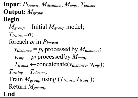
Using GAMC, M_group is obtained. In particular, M_group accepts the image encoding (compressed image vector and distance vector) of a ground plot image as an input and generated the corresponding cluster assignment vector v_encode as an output. Thereafter, V_encode can be used as critical data to identify plots with similar SLD trends.In the process of obtaining M_group, SELF-HE employs an adaptive number of categories. The SLD-E algorithm of SELF-HE prespecifies a number of categories N_category that significantly exceed the actual required number. After processing using M_sldcluster for T_cluster, the dimensions of several categories do not exceed the value of other dimensions (cannot be represented as a category label in the results); thus, the number of categories finally obtained is significantly lower than N_category. The actual number of classifications obtained by M_group is then as follows:

$N_{real-category}=Count\left(Unique\left(ArgMax(T_{\mathit{cluser}},0)\right)\right),(7)$

where ArgMax returns indices of the maximum values along an axis, Unique returns unique elements of an array, and Count returns the number of elements.

High-Level Encoding and SLF

When M_cmp, M_distance, and M_group have been obtained, M_encode can be constructed. The inputs into M_encode are the image patch and area information, and the output is the high-level encoding vector v_encode. Based on v_encode, an SLF model is constructed. The corresponding process is shown in Figure 5.

FIGURE 5

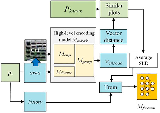
FIGURE 5. M_encode and SLF model development.

As shown in Figure 5, M_encode is constructed from M_cmp, M_distance, and M_group. Moreover, M_cmp accepts image patch data and generates v_cmp, and M_distance accepts location information as an input to generate v_distance. Finally, v_cmp and v_distance are concatenated and input into M_group to generate the model output v_encode. Through this process, M_encode can realize the end-to-end capacity to encode the information of individual plots, and the resulting encoding can be further used to establish an SLF model.

Through M_encode, all plots in P_known can be processed to obtain the encoding results V_known = {v₁, v₂, … , v_n}. For plot p_x, for which an SLF model should be obtained, the corresponding image patch I_x is then cut from Z in accordance with its area attribute, and p_x.area and I_x are input into M_encode to obtain v_encode. For two encoding vectors, the distance between them is as follows:

$distance\left(v_1,v_2\right)=l1norm(v_1-v_2).(8)$

Based on Eq. 8, the m nearest vectors in V_known can be identified using the k-NN algorithm; thus, the most similar plots in known, that is, similar = {p₁, p₂, … , p_m}, can be identified. The average SLD, as denoted by averageSLD, is calculated as follows:

$averageSLD\left(Similar\right)=\frac{{{\displaystyle \sum }}_i^m{p}_i.SLD}{m}.(9)$

Accordingly, averageSLD represents the variation trend and fluctuation range of the electric load data of p_x. Although insufficient historical data are available for p_x, these data can provide the range of load changes within a period. Thereafter, based on the load change interval INT of p_x.history, long-term historical data can be estimated by calculating longhistory = INT × averageSLD, which can further support the development of M_forecast.

After all the above-mentioned steps, we finally obtain an end-to-end deep neural network model M_encode that can be used as a bridge from ground-building features to electrical load characteristics. Moreover, the remote sensing image data and location information of a plot are input into M_encode, which then produces high-level encoding corresponding to the image. This code can be used to identify the most similar plots with rich historical electrical load data and subsequently to obtain the average SLD. For the current plot, the average SLD can supplement the shortcomings of the insufficient data and obtain forecasting M_forecast, which is more stable and accurate than using the historical data of the plot. Finally, electrical power forecasting for developing regions or regions lacking historical load data could be realized.

Experiments and Results

Method Realization and Study Area

We adopted Python to implement the SELF-HE method and all methods considered for comparison, and TensorFlow was used to develop the deep neural network models in SELF-HE. All experiments were performed on a computer with an Intel Core i9-9900K CPU, a GeForce RTX 2080 11 GB graphics processing unit (GPU), and 64 GB of memory.

The target area in this study corresponds to the northern area of the city of Changchun, Jilin Province, China. This area is a rapidly growing area of Changchun, and methods such as SELF-HE are required to provide decision support for SLF. This area is shown in Figure 6.

FIGURE 6

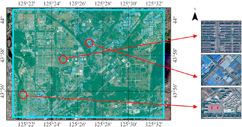
FIGURE 6. Study area and the corresponding remote sensing images.

The target area and SLF Zone Z marked in Figure 6 contained various commercial, residential, educational, and manufacturing areas, all of which exhibited significantly different electrical load characteristics. The high-resolution remote sensing images of the study area were not obtained from a single remote sensing satellite sensor. In particular, we used the ArcGIS Living Atlas “World Image” web map service as the data source. For Zone Z in the study area, this service can provide detailed remote sensing image information from Level 0 to 23. We selected the 17th level, at which the resolution was 1.19 m per pixel, which was sufficient to distinguish the structural characteristics of ground objects and could support the process of SELF-HE. Different regions in Z exhibited typical differences in structure and morphology, and these differences were used as critical clues to identify plots with similar SLDs.

For the electrical load data, we selected 640 plots with dimensions of 300 × 300 m and collected historical electric load data from ammeters in the corresponding plots. The plots are shown in Figure 7.

FIGURE 7

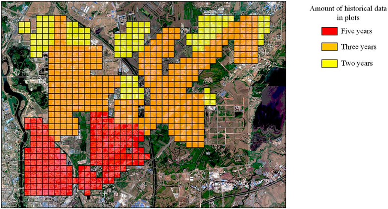
FIGURE 7. Plots and amount of historical data.

As shown in Figure 7, these plots can be divided into three categories, the details of which are listed below.

Five Years

Five years of historical data were available from 2016 to 2020. The corresponding area was developed relatively early; thus, the data were relatively rich, and 170 plots belonged to this category.

Three Years

Three years of historical data were available from 2018 to 2020; several accumulated electrical load data were available for this area, and 351 plots belonged to this category.

Two Years

Only 2 years of historical data were available from 2019 to 2020. These plots belonged to a newly developed area, for which there were insufficient historical data; and 119 plots belonged to this category.

Among all the above-mentioned plots, 50% of the plots in categories 1) and 2) were randomly selected as the SLD source dataset. This dataset consisted of historical data from 2016 to 2019 and did not contain data from 2020. The 2020 data for all the plots were used to construct the test set, which was further divided into three subsets, as follows. Test set 1 corresponded to the remaining 50% of the 5-years plots, Test set 2 corresponded to the remaining 50% of the 3-year plots, and Test set 3 corresponded to all 2-year plots.

Methods Considered for Comparison

To evaluate the load forecasting capacity of SELF-HE, the following methods were considered for comparison in this study.

Forecasting Model Trained Using Historical Data (F-History)

For all test sets, all data except those from 2020 were used to train the forecasting model. For this model, the SLD dataset was not required. Moreover, F-History uses an LSTM network as a forecasting model, and the forecasting time period is 7 days (when forecasting the load for the following 7 days at a certain time point, the load data generated in the previous 7 days are required as input).

Nearest Matching SLD (Nearest-SLD)

For an unknown plot p_x, the plot in the SLD source dataset that was the closest to p_x was used to train the same LSTM forecasting model as in F-History based on the corresponding SLD information.

K-Neighbor Matching SLD (Neighbor-SLD)

For an unknown plot p_x, the k plots in the SLD source dataset that were the closest to p_x were identified, and their average SLD was obtained to develop the forecasting model.

Structural Similarity Matching SLD (Similar-Structure)

M_cmp from SELF-HE was used to extract v_cmp for each plot; v_cmp was used as a metric to determine the best-matching plot in the SLD source dataset, and its SLD was then used to construct a forecasting model.

SELF-HE

The method proposed in this study.

The prediction models used in each of the five methods above exhibit the same structure. Consequently, the capacity to adapt to different data characteristics and historical data volumes has a significant influence on the accuracy of the results. To evaluate the forecasting accuracy of each of the five methods for a given plot, we used the error rate defined below:

$ErrorRate\left(Plot\right)=\frac{{\displaystyle {\sum }_{d=1}^m\frac{|Forecas{t}_m-Rea{l}_m|}{Rea{l}_m}}\times 100\%}{m}.(10)$

This equation measures the 1-to-m-day forecasting error for a plot, where Forecast_m represents the forecasting result on the mth day, and real_m represents the true load on the mth day. For the entire test set, the prediction error was as follows:

$AverageErrorRate\left(set\right)=\frac{{\displaystyle {\sum }_{i=1}^{n}ErrorRate\left(Plo{t}_i\right)}}{n}.(11)$

This average error rate represents the average forecasting error for all plots in a set of test data. As the value increases, the error increases. In this study, the average error rate was used to measure the forecasting capacity of each method.

Details of the SELF-HE Clustering Results and Comparison of the Average Error Rates of the Five Methods

The SELF-HE method comprises multiple steps. The SLD-E algorithm in Step 2 performs cluster encoding based on SLD and spatial distance, and typical clustering results are shown in Figure 8.

FIGURE 8

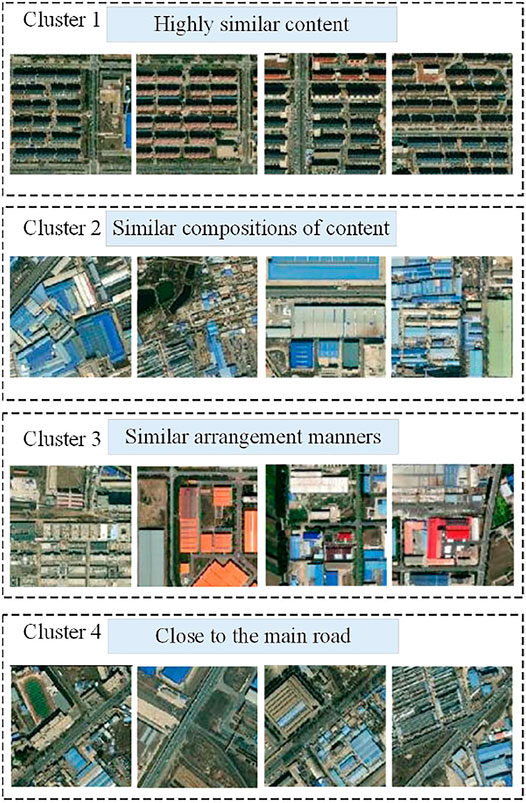
FIGURE 8. Clustering results of SLD-E.

Figure 8 presents several examples of the typical clustering results of the SLD-E algorithm. The clustering results were obtained using SLD and spatial distance as criteria (the image content was not considered in the clustering process). However, as can be seen from the resulting clusters, plots in the same cluster exhibit similar spatial characteristics. Cluster 1 consists of residential areas that are highly similar in structural scale (size) and arrangement, and the patterns of electricity consumption in these areas are highly similar. For Cluster 2, although the sizes and directions are different, the plots correspond to the production workshops of small enterprises and exhibit similar compositions of content. The plots in Cluster 3 are from commercial areas and display similar patterns of arrangement. For the plots in Cluster 4, although their contents are not the same, they are all close to the main road. As can be seen from the results, the approximation of the SLD is correlated with the spatial characteristics of the remote sensing images. However, the mode of this correlation is not unique, and the four clusters correspond to four different correlation modes. Therefore, pure image approximation cannot describe all relevant relationships, and a more effective method, such as the GAMC algorithm of SELF-HE, is required to describe these relationships.

The average error rates of the five methods are shown in Table 1. As can be seen from this table, F-History does not use the SLD source dataset and relies only on the historical data in the test set to build a forecasting model. Moreover, given that Test set 1 contains 4 years of historical data, F-History reaches its optimal forecasting accuracy using this test set. The accuracy of this method rapidly declines as the amount of available historical data decreases, and the poorest result is obtained for Test set 3, with an average error rate of 17.12%. It can be seen that a reduction in the amount of historical data has a significant influence on the forecasting model. For Nearest-SLD and Neighbor-SLD, the spatial distance was used as the criterion for selecting the SLD information from P_known. For Test sets 1 and 2, these methods yield lower accuracies than F-History. However, for Test set 3, the results are superior to those of F-History, indicating that Nearest-SLD and Neighbor-SLD have positive influences on the load forecasting when the available historical data are limited. Similar-Structure used the similarity of image characteristics to identify plots with similar SLDs in known, and the trend of the results obtained using this method is similar to those of Nearest-SLD and Neighbor-SLD, with an accuracy slightly lower than that of Neighbor-SLD. Among all the methods, SELF-HE achieves the best results. For Test set 1, the average error rate of 4.23% is the lowest result obtained; for Test set 3, with only 1 year of historical load data, the average error rate of 8.14% is superior to those of the other methods. A comparison of the performance of the five methods is presented in Figure 9.

TABLE 1

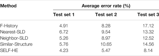
TABLE 1. Average error rates of the five methods.

FIGURE 9

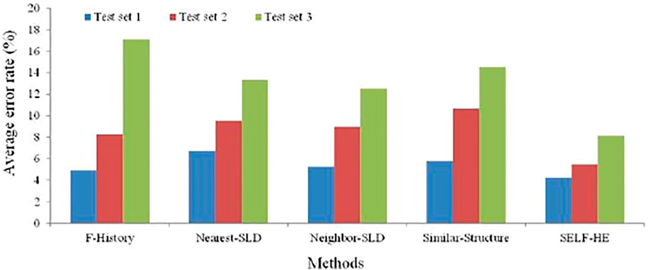
FIGURE 9. Comparison of the five methods.

As shown in Figure 9, for all data sets, the SELF-HE method achieves the lowest average error rate, and Neighbor-SLD is superior to the other three methods. Moreover, F-History has the least significant influence on the test set with the smallest amount of data. Test set 1 contains 5 years of historical data, and the electricity consumption behavior of the corresponding plots is relatively stable. Based on Test set 1, using 1 year (2019), 2 years (2018 and 2019), 3 years (2017–2019), and 4 years (2016–2019) of historical data, the average error rates achieved by the five methods are listed in Table 2.

TABLE 2

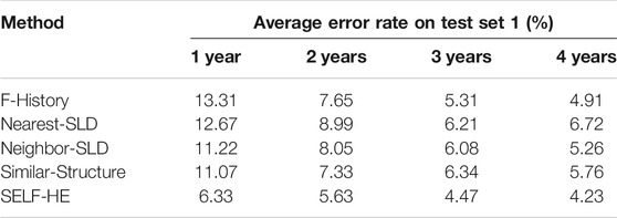
TABLE 2. Average error rate using Test set 1.

The corresponding trends of the average error rate with respect to the historical data volume shown in Table 2 are illustrated in Figure 10.

FIGURE 10

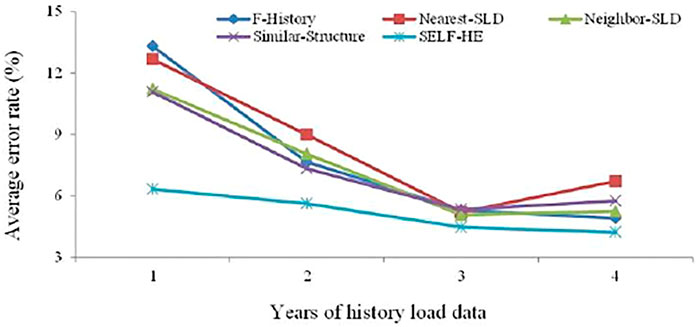
FIGURE 10. Trends of average error rate with respect to the historical data volume.

Given that the plots in Test set 1 (from the older urban areas) have the longest available history, their electricity consumption characteristics are more stable than those for the other test sets. Consequently, the 1-year results in Table 2 are superior to the results for Test set 3 in Table 1. As shown in Table 1 and Figure 10, as the amount of historical data increases, the average error rates of all the methods decrease. The decreasing trend of F-History is the most significant, indicating that this method is highly dependent on the amount of historical data. Moreover, F-History requires more historical data than other methods to develop the forecasting model and demonstrates improved performance when there are abundant historical data, and the electricity consumption behavior for the corresponding plots is stable. However, for newly developed areas in a city, sufficient historical data were not available, and the electricity consumption behavior of users corresponding to those plots was not sufficiently stable (e.g., several companies had not started running their machines). These problems prevented F-History from achieving high performance in the SLF. As observed, Nearest-SLD exhibits an unstable trend from three to 4 years, with an increase in the amount of historical data, leading to a slight increase in the average error rate; whereas the trends of Neighbor-SLD and Similar-Structure are more stable. Since the Z is located in a rapid development region of city, many plots’ corresponding supporting facilities have been built in just recent years, and some companies have undergone industrial transformation and renovation; this may lead to huge differences in the characteristics of historical data that are far apart in time. At this time, if a larger amount of data is introduced from a single neighbor (whether in distance, distribution, or structure), it may lead to the introduction of too much heterogeneity information and reduce the accuracy; so errors increase for Nearest-SLD, Neighbor-SLD, and Similar-Structure in Figure 10. Among all the methods, the trend of SELF-HE is the most gradual, and the results obtained using only 2 years of historical data are similar to the results of the other methods using 4 years of data.

Using SLDs to supplement the lack of historical data can improve the performance of an SLF model. The Nearest-SLD algorithm uses a known plot from among the neighbors of the plot of interest as the source of the SLD information. This strategy can achieve higher performance than F-History; however, due to the extensive distribution of boundaries between different land use areas in cities, the use of the plot in the nearest position may cause an increase in error. Hence, Nearest-SLD is not stable. To address this shortcoming, Neighbor-SLD uses multiple known plots from among the neighbors of the plot of interest as the SLD source, achieving higher and more stable performance than Nearest-SLD. The concept of Similar-Structure is consistent with that of SELF-HE. In particular, the similarity between the features of remote sensing images is used as the standard for identifying plots with similar SLDs. However, as can be seen from Figure 8, the spatial characteristics defining an SLD cluster do not necessarily follow a uniform rule; as distinct spatial arrangements, adjoining relationships, and content compositions may all be commonalities that define SLD clusters. Given that Similar-Structure uses only the vector distance based on v_cmp as the standard for assessing similarity, it may be suitable only for cases analogous to that of Cluster 1 in Figure 8, and it may not readily adapt to other cases. Similar-Structure exhibits no significant advantage over Nearest-SLD or Neighbor-SLD. Among all the methods, the trend of SELF-HE is the most gradual, and the results obtained using only 2 years of historical data are similar to those of the other methods using 4 years of historical data.

To analyze comprehensively the processes by which the SLF is obtained using each method, we selected a typical plot in the northeast corner of Z as the unknown plot P_x; the process of each algorithm is shown in Figure 11.

FIGURE 11

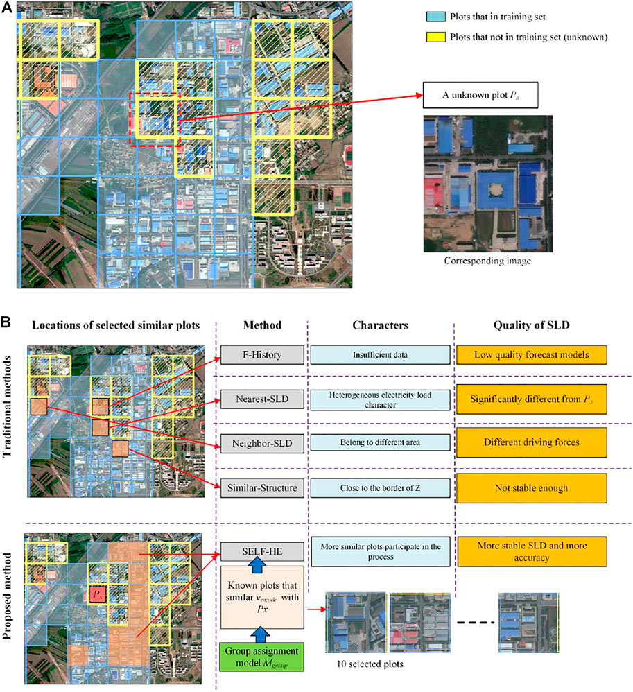
FIGURE 11. Detailed process of each method: (A) unknown plot P_x and (B) comparison of all the methods.

As shown in Figure 11A, there are two types of plots in this area. The plots indicated in blue are from the training set; their SLD is stable and contains more historical data. The plots indicated in yellow are from the testing set, and they contain less historical data. Given that P_x is an unknown plot from the testing set, additional SLD data may be required to facilitate its SLF calculation. The characteristics of the five methods are shown in Figure 11B, and the error rates of the five methods on P_x are listed in Table 3.

TABLE 3

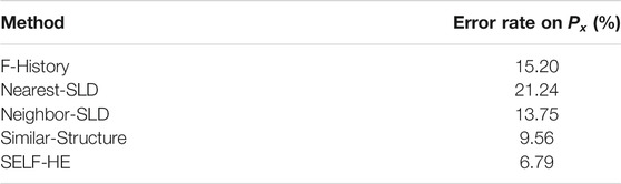
TABLE 3. Error rates of the five methods on P_x.

For F-History, as it only uses limited historical data for SLF calculations, the plots of the neighbors do not participate in the SLF calculation. Moreover, due to the lack of historical data, the SLF model generated by F-History is readily fitted with specific features, which reduces its prediction accuracy. The error rate of F-History is 15.20%. For Nearest-SLD, there are four plots closest to P_x (east, south, west, and north). Given that the north and east are unknown plots, only west or east can be selected. The Nearest-SLD algorithm finally selected the south plot as the source of SLD. Although this selection mitigates the lack of historical data in F-History, this plot is located at the junction of residential and industrial areas, and its load consumption characteristic is significantly different from that of P_x, leading to the introduction of heterogeneous SLD. Thus, the forecast results obtained are lower than those of F-History, and its error rate is the highest, at 21.24%. The Nearest-SLD algorithm uses SLD to identify similar plots. As can be seen from Figure 11B, Nearest-SLD identified a plot across the main road. Although this plot can help P_x obtain the SLD and improve the accuracy of the forecast; in urban environments, several main roads divide different administrative regions, functional regions, enterprises, or residential structures in the city, which results in different policies and groups that are core driving forces of power consumption. The Nearest-SLD error rate is 13.75%. Similar-Structure selected a plot with a similar building structure and composition content near P_x. The SLD provided by this plot causes the error rate of Similar-Structure to reach 9.56%, indicating that it is feasible to use the structure of the ground building as an index to obtain the SLD. However, this method exhibits several problems. In particular, for this plot in the rapid urban development area, the electricity consumption characteristics are not sufficiently stable; thus, further improvement is required. Moreover, SELF-HE uses M_group to assign v_encode to all plots and then selects the 10 most similar plots. Based on the average SLD of these plots, the optimal result obtained by SELF-HE demonstrates an error rate of 6.79%. This result indicates that the SELF-HE electric load forecasting based on the high-level encoding of high-resolution remote sensing images is more effective than those of the other methods. Moreover, SELF-HE achieves the optimal results among the five methods, indicating that it can extract key characteristics for SLD clustering in remote sensing images and acquire SLDs that are highly similar to the SLD of a plot of interest, enabling more accurate and stable forecasting results to be obtained. The corresponding results reveal that SELF-HE can foster connections between different remote sensing image characteristics (e.g., the specific characteristics described in Figure 8) and SLD selection, which can serve as a new data source for SLF.

Comparison of Methods Under Different Scenarios

To more fully evaluate the spatial forecasting ability of SELF-HE under different scenarios, we introduce more regions for comparison, and the characteristics of these regions are as follows.

Stable old urban region (SO-R).

The central part of Changchun City is selected as the research object. This area has been developed for decades, and the number and type of residents and enterprises are relatively stable.

The changing old urban region (CO-R).

A region of Jilin City was selected as the research object. The original industry in this region was concentrated in the chemical field, and now it is transforming into the green and high-tech field.

Rapidly developing area with relatively monotonous industry (DM-R).

Select a developing region in Tonghua City, and the enterprises in this region are mainly concentrated in the pharmaceutical field.

Rapidly developing areas combining various industries (DV-R).

The economic and technological development zone of Changchun City is selected as the object, and the enterprises in this area come from various fields.

For the above four test scenarios, we tested the error rates of the five methods, and the comparison is shown in Table 4.

TABLE 4

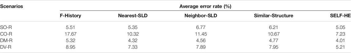
TABLE 4. Comparison of the methods under different scenarios.

It can be seen from Table 4 that for scenario SO-R, all five methods have achieved good results due to the relatively stable electric load character, and SELF-HE is slightly better than the other four methods. For CO-R, the large amount of historical data becomes unreliable because the region is in industrial restructuring, and F-History achieves the worst results due to its high dependence on historical data. For DM-R, due to the monotonous industrial structure, the prediction is relatively easy, and the five methods have obtained good results. For DV-R, the accuracy drops due to the heterogeneity of electricity users in the region. SELF-HE has obtained the best results for the above four scenarios, indicating that SELF-HE has good stability and can adapt to various spatial forecast work; especially for CO-R and DV-R the advantages of the proposed method are more obvious, indicating that SELF-HE can cope with the changes and diversity of electric users in a region and can obtain higher-precision forecasting results.

Further Research

The separate strategy of plots has a considerable impact on SELF-HE. Smaller plots will make the SLF results more capable of reflecting the characteristics of urban regions, but it will also increase the fluctuation of the load data in the boundaries between different regions and reduce the SLF accuracy. Meanwhile, larger plots will introduce more objects and make the load data more stable, but they will confuse the content of different regions and reduce the value of the SLF result. In this study, the plot size was manually specified; this strategy may not yield the optimal solutions and may cause a longer trial-and-error experimental process. In future research, we plan to introduce more urban data sets and plot sizes to explore the relationships between different urban areas and a variety plot sizes and then explore ways to optimize the plot size automatically to make SELF-HE more efficient.

Conclusion

For the SLF process, considerable historical data are typically required to construct forecasting models. As it is generally difficult to accumulate sufficient data for rapidly developing regions in cities, considering the SLD information of plots for which abundant historical data are available is a feasible solution. With this approach, the key is to find plots with electricity consumption behaviors that are similar to that of the plot to be predicted.

To this end, this study proposes a spatial electric load forecasting method based on the high-level encoding of high-resolution remote sensing images called SELF-HE. Based on the experimental results, when the plots contained relatively small amounts of historical data, the traditional F-History approach could not achieve high accuracies, and the Nearest-SLD method could be influenced by the boundaries of different land use categories, introducing errors into the forecasting results. Owing to the diversity of historical data and ground data, a selection strategy that only relies on SLD (Neighbor-SLD) or ground object features (Similar-Structure) cannot fully represent the characteristics of the plot to be predicted; thus, the prediction results are unstable. Moreover, SELF-HE adopts high-resolution remote sensing images as a data source for the identification of similar plots, which enables the direct use of remote sensing images to obtain more appropriate SLD estimates. Thus, SELF-HE achieved the optimal results among the five methods.

Furthermore, SELF-HE bridges the remote sensing features and electric load characteristics and enables SLF to be performed based on remote sensing, to obtain higher-quality electric load forecasting results at a lower data collection cost. Using SELF-HE, load forecasting results for larger regions or areas of new development can, therefore, be rapidly obtained, which play an important role in the field of regional power infrastructure construction planning and power grid management.

Data Availability Statement

The original contributions presented in the study are included in the article/Supplementary Material, further inquiries can be directed to the corresponding author.

Author Contributions

BW: writing and method. HS: idea and proof.

Funding

This work was supported in part by the Scientific and Technological Planning Project of Jilin Province (20190302106GX).

Conflict of Interest

The authors declare that the research was conducted in the absence of any commercial or financial relationships that could be construed as a potential conflict of interest.

Publisher’s Note

All claims expressed in this article are solely those of the authors and do not necessarily represent those of their affiliated organizations, or those of the publisher, the editors, and the reviewers. Any product that may be evaluated in this article, or claim that may be made by its manufacturer, is not guaranteed or endorsed by the publisher.

References

Brunoro, C. M., El Hage, F. S., and de Oliveira, C. C. B. (2009). “Integrated Model of Spatial and Global Load Forecast for Power Distribution Systems,” in 20th International Conference and Exhibition on Electricity Distribution-Part 1 (CIRED, 2009 IET), 1–4.

CrossRef Full Text | Google Scholar

Carreno, E. M., Rocha, R. M., and Padilha-Feltrin, A. (2010). A Cellular Automaton Approach to Spatial Electric Load Forecasting. IEEE Trans. Power Syst. 26, 532–540.

Google Scholar

Chakraborty, T., Lee, X., Ermida, S., and Zhan, W. (2021). On the Land Emissivity assumption and Landsat-Derived Surface Urban Heat Islands: A Global Analysis. Remote Sensing Environ. 265, 112682. doi:10.1016/j.rse.2021.112682

CrossRef Full Text | Google Scholar

Chow, J. H., Wu, F. F., and Momoh, J. A. (2005). “Applied Mathematics for Restructured Electric Power Systems,” in Applied Mathematics for Restructured Electric Power Systems (Springer), 1–9.

Google Scholar

Evangelopoulos, V., Karafotis, P., and Georgilakis, P. (2020). Probabilistic Spatial Load Forecasting Based on Hierarchical Trending Method. Energies 13, 4643. doi:10.3390/en13184643

CrossRef Full Text | Google Scholar

Georgilakis, P. S., and Hatziargyriou, N. D. (2015). A Review of Power Distribution Planning in the Modern Power Systems Era: Models, Methods and Future Research. Electric Power Syst. Res. 121, 89–100. doi:10.1016/j.epsr.2014.12.010

CrossRef Full Text | Google Scholar

Han, Z., Cheng, M., Chen, F., Wang, Y., and Deng, Z. (2020). A Spatial Load Forecasting Method Based on DBSCAN Clustering and NAR Neural Network. J. Phys. Conf. Ser., 1449. IOP Publishing, 012032. doi:10.1088/1742-6596/1449/1/012032

CrossRef Full Text | Google Scholar

He, Y. X., Zhang, J. X., Xu, Y., Gao, Y., Xia, T., and He, H. Y. (2015). Forecasting the Urban Power Load in China Based on the Risk Analysis of Land-Use Change and Load Density. Int. J. Electr. Power Energ. Syst. 73, 71–79. doi:10.1016/j.ijepes.2015.03.018

CrossRef Full Text | Google Scholar

Hung-Chih Wu, H. C., and Chan-Nan Lu, C. N. (2002). A Data Mining Approach for Spatial Modeling in Small Area Load Forecast. IEEE Trans. Power Syst. 17, 516–521. doi:10.1109/tpwrs.2002.1007927

CrossRef Full Text | Google Scholar

Kang, J., Fernandez-Beltran, R., Hong, D., Chanussot, J., and Plaza, A. (2020). Graph Relation Network: Modeling Relations between Scenes for Multilabel Remote-Sensing Image Classification and Retrieval. IEEE Trans. Geosci. Remote Sensing. 59, 4355–4369.

Google Scholar

Li, M., Stein, A., Bijker, W., and Zhan, Q. (2016). Urban Land Use Extraction from Very High Resolution Remote Sensing Imagery Using a Bayesian Network. ISPRS J. Photogrammetry Remote Sensing 122, 192–205. doi:10.1016/j.isprsjprs.2016.10.007

CrossRef Full Text | Google Scholar

Li, W., Liu, H., Wang, Y., Li, Z., Jia, Y., and Gui, G. (2019). Deep Learning-Based Classification Methods for Remote Sensing Images in Urban Built-Up Areas. IEEE Access 7, 36274–36284. doi:10.1109/access.2019.2903127

CrossRef Full Text | Google Scholar

Melo, J., Carreno, E., and Padilha-Feltrin, A. (2012). “Considering Urban Dynamics in Spatial Electric Load Forecasting,” in IEEE Power Energy Soc. Gen. Meet. (IEEE Publications), 1–7. doi:10.1109/pesgm.2012.6345436

CrossRef Full Text | Google Scholar

Melo, J., Carreno, E., and Padilha-Feltrin, A. (2010). “Spatial Load Forecasting Using a Demand Propagation Approach,” in (IEEE Publications)/PES Transmission and Distribution Conference and Exposition (Latin America T&D-LA), 196–203. doi:10.1109/tdc-la.2010.5762882

CrossRef Full Text | Google Scholar

Melo, J. D., Carreno, E. M., Calviño, A., and Padilha-Feltrin, A. (2014). Determining Spatial Resolution in Spatial Load Forecasting Using a Grid-Based Model. Electric Power Syst. Res. 111, 177–184. doi:10.1016/j.epsr.2014.02.019

CrossRef Full Text | Google Scholar

Melo, J. D., Carreno, E. M., and Padilha-Feltrin, A. (2015). Estimation of a Preference Map of New Consumers for Spatial Load Forecasting Simulation Methods Using a Spatial Analysis of Points. Int. J. Electr. Power Energ. Syst. 67, 299–305. doi:10.1016/j.ijepes.2014.11.023

CrossRef Full Text | Google Scholar

Monteiro, C., Ramirez-Rosado, I. J., Miranda, V., Zorzano-Santamaria, P. J., Garcia-Garrido, E., and Fernandez-Jimenez, L. A. (2005). GIS Spatial Analysis Applied to Electric Line Routing Optimization. IEEE Trans. Power Deliv. 20, 934–942. doi:10.1109/tpwrd.2004.839724

CrossRef Full Text | Google Scholar

Moreno-Carbonell, S., Sánchez-Úbeda, E. F., and Muñoz, A. (2020). Rethinking Weather Station Selection for Electric Load Forecasting Using Genetic Algorithms. Int. J. Forecast. 36, 695–712. doi:10.1016/j.ijforecast.2019.08.008

CrossRef Full Text | Google Scholar

Pan, X., Zhang, C., Xu, J., and Zhao, J. (2021). Simplified Object-Based Deep Neural Network for Very High Resolution Remote Sensing Image Classification. ISPRS J. Photogrammetry Remote Sensing 181, 218–237. doi:10.1016/j.isprsjprs.2021.09.014

CrossRef Full Text | Google Scholar

Park, S.-J., Lee, C.-W., Lee, S., and Lee, M.-J. (2018). Landslide Susceptibility Mapping and Comparison Using Decision Tree Models: A Case Study of Jumunjin Area, Korea. Remote Sensing 10, 1545. doi:10.3390/rs10101545

CrossRef Full Text | Google Scholar

Plant, G., Kort, E. A., Murray, L. T., Maasakkers, J. D., and Aben, I. (2022). Evaluating Urban Methane Emissions from Space Using TROPOMI Methane and Carbon Monoxide Observations. Remote Sensing Environ. 268, 112756. doi:10.1016/j.rse.2021.112756

CrossRef Full Text | Google Scholar

Pristeri, G., Peroni, F., Pappalardo, S. E., Codato, D., Masi, A., and De Marchi, M. (2021). Whose Urban green? Mapping and Classifying Public and Private green Spaces in Padua for Spatial Planning Policies. Ijgi 10, 538. doi:10.3390/ijgi10080538

CrossRef Full Text | Google Scholar

Salvó, G., and Piacquadio, M. N. (2017). Multifractal Analysis of Electricity Demand as a Tool for Spatial Forecasting. Energy Sustain. Dev. 38, 67–76.

Google Scholar

Shi, K., Chen, Y., Yu, B., Xu, T., Yang, C., Li, L., et al. (2016). Detecting Spatiotemporal Dynamics of Global Electric Power Consumption Using DMSP-OLS Nighttime Stable Light Data. Appl. Energ. 184, 450–463. doi:10.1016/j.apenergy.2016.10.032

CrossRef Full Text | Google Scholar

Shin, J.-H., Yi, B.-J., Kim, Y.-I., Lee, H.-G., and Ryu, K. H. (2011). Spatiotemporal Load-Analysis Model for Electric Power Distribution Facilities Using Consumer Meter-reading Data. IEEE Trans. Power Deliv. 26, 736–743. doi:10.1109/tpwrd.2010.2091973

CrossRef Full Text | Google Scholar

Srivastava, S., Vargas-Muñoz, J. E., and Tuia, D. (2019). Understanding Urban Landuse from the above and Ground Perspectives: A Deep Learning, Multimodal Solution. Remote Sensing Environ. 228, 129–143. doi:10.1016/j.rse.2019.04.014

CrossRef Full Text | Google Scholar

Su, Y., Zhong, Y., Zhu, Q., and Zhao, J. (2021). Urban Scene Understanding Based on Semantic and Socioeconomic Features: From High-Resolution Remote Sensing Imagery to Multi-Source Geographic Datasets. ISPRS J. Photogrammetry Remote Sensing 179, 50–65. doi:10.1016/j.isprsjprs.2021.07.003

CrossRef Full Text | Google Scholar

Vasquez-Arnez, R., Jardini, J., Casolari, R., Magrini, L., Semolini, R., and Pascon, J. (2008). “A Methodology for Electrical Energy Forecast and its Spatial Allocation over Developing Boroughs,” in (IEEE Publications)/PES Transmission and Distribution Conference and Exposition, 1–6.

CrossRef Full Text | Google Scholar

Willis, H. L. (2002). Spatial Electric Load Forecasting. Florida: CRC Press.

Google Scholar

Willis, H., and Tram, H. (1983). A Cluster Based V.A.I. Method for Distribution Load Forecasting. IEEE Trans. Power Apparatus Syst. PAS-102, 2677–2684. doi:10.1109/tpas.1983.317673

CrossRef Full Text | Google Scholar

Xie, S., Hu, Z., Zhou, D., Li, Y., Kong, S., Lin, W., et al. (2018). Multi-objective Active Distribution Networks Expansion Planning by Scenario-Based Stochastic Programming Considering Uncertain and Random Weight of Network. Appl. Energ. 219, 207–225. doi:10.1016/j.apenergy.2018.03.023

CrossRef Full Text | Google Scholar

Yao, W., Chung, C. Y., Wen, F., Qin, M., and Xue, Y. (2015). Scenario-based Comprehensive Expansion Planning for Distribution Systems Considering Integration of Plug-In Electric Vehicles. IEEE Trans. Power Syst. 31, 317–328.

Google Scholar

Ye, C., Ding, Y., Wang, P., and Lin, Z. (2019). A Data-Driven Bottom-Up Approach for Spatial and Temporal Electric Load Forecasting. IEEE Trans. Power Syst. 34, 1966–1979. doi:10.1109/tpwrs.2018.2889995

CrossRef Full Text | Google Scholar

Ying, L.-C., and Pan, M.-C. (2008). Using Adaptive Network Based Fuzzy Inference System to Forecast Regional Electricity Loads. Energ. Convers. Manage. 49, 205–211. doi:10.1016/j.enconman.2007.06.015

CrossRef Full Text | Google Scholar

Yuan, H., Yang, G., Li, C., Wang, Y., Liu, J., Yu, H., et al. (2017). Retrieving Soybean Leaf Area index from Unmanned Aerial Vehicle Hyperspectral Remote Sensing: Analysis of RF, ANN, and SVM Regression Models. Remote Sensing 9, 309. doi:10.3390/rs9040309

CrossRef Full Text | Google Scholar

Zhang, C., Wei, S., Ji, S., and Lu, M. (2019). Detecting Large-Scale Urban Land Cover Changes from Very High Resolution Remote Sensing Images Using CNN-Based Classification. Ijgi 8, 189. doi:10.3390/ijgi8040189

CrossRef Full Text | Google Scholar