Gab-SSDS: An AI-Based Similar Days Selection Method for Load Forecast

The important, while mostly underestimated, step in the process of short-term load forecasting–STLF is the selection of similar days. Similar days are identified based on numerous factors, such as weather, time, electricity prices, geographical conditions and consumers’ types. However, those factors influence the load differently within different circumstances and conditions. To investigate and optimise the similar days selection process, a new forecasting method, named Genetic algorithm-based–smart similar days selection method–Gab-SSDS, has been proposed. The presented approach implements the genetic algorithm selecting similar days, used as input parameters for the STLF. Unlike other load forecasting methods that use the genetic algorithm only to optimise the forecasting engine, authors suggest additional use for the input selection phase to identify the individual impact of different factors on forecasted load. Several experiments were executed to investigate the method’s effectiveness, the forecast accuracy of the proposed approach and how using the genetic algorithm for similar days selection can improve traditional forecasting based on an artificial neural network. The paper reports the experimental results, which affirm that the use of the presented method has the potential to increase the forecast accuracy of the STLF.

1 Introduction

World’s limited energy sources influence the global electric power industry and constrain the energy demand, which varies daily. An accurate electrical load prediction is a necessity, and it plays a crucial role in the coordination of power generation (Khwaja et al., 2015). Therefore, a precise load forecast is acquired by utilities and system operators in order to provide efficient unit commitment, load dispatching decisions, contingency planning, and optimal load flow (Campillo et al., 2012; Kavousi-Fard et al., 2014).

Forecasting the electrical load from one to several days ahead is usually referred to as short-term load forecasting–STLF. It is one of the critical parameters that help electrical utility operators make decisions regarding purchasing and selling electric power, maintenance, load switching, and maintenance planning, including some sophisticated areas, e.g., as relay protection (Selakov et al., 2014). In a deregulated electricity market, STLF is a helpful tool for the economical and reliable operation of the power system. The primary application of STLF is to provide load predictions for generation scheduling, such as unit commitment and economic dispatch (Li et al., 2016). In addition, STLF is an essential component of smart grids for cost savings and ensuring a continuous flow of electricity supply (Khwaja et al., 2015; Berntzen et al., 2021) and generating operating decisions such as dispatch scheduling, maintenance plans and security analysis(Kyriakides and Polycarpou, 2007; Kouhi et al., 2014; Çevik and Çunkaş, 2015). Therefore, STLF plays a significant role in distribution and transmission planning, maintenance, and scheduling.

Various methods and load forecasting techniques have been proposed and applied in load forecasting. However, there is still an essential need for a more accurate load forecast since a universal forecasting solution cannot be made that will give the most accurate results for all areas and weather conditions (Selakov et al., 2014). The critical step in the process that is underestimated chiefly is the similar days selection. The selection of similar days can improve the identification of patterns in the forecasting process, and it can be combined with many forecasting techniques. For example, forecasting based on linear regression or artificial neural network requires adequate training data with a strong relationship between the predictor and predicted data. Such adequate input can be achieved by selecting days from history similar enough to forecasting day. The similar days identification is based on numerous similarity factors, such as weather, time, characteristics of population, economy, electricity prices, geographical conditions, and type of consumers (Khwaja et al., 2015). However, these factors influence the load differently within different circumstances and condition sets. For example, the influence of outside temperature on the load pattern varies depending on other factors such as the day in a week, time of day, wind speed, sky cover, or more specific ones: load inertia and daylight duration. Therefore, in similar days selection, every specific factor should be assigned with proper weight, depending on the particular circumstances, representing its impact at a specific point in time. Poor initialisation of those weights may introduce inferior values, leading to an unreliable result. In order to address the variety of factors and differences in their influence on forecasting, additional methods should be introduced to improve the calculation (Barman et al., 2018; Karimi et al., 2018). Therefore, the authors identified a need for a meta-heuristic technique to optimise weight coefficients for the selection of similar days, and suggested a method that addresses the issues mentioned above, using a genetic algorithm (GA). The genetic algorithm was chosen because of its ability to converge to the globally optimal result since it has an efficient exploration ability to search in the global scope of the search space (Lipo Wang, 2010). The optimal result is achieved by mutation schemes which tend to increase diversity among the population (Simon, 2008), and escape a convergence to some of the local minimums. Such an approach is essential in systems with many different input variables that can be optimised.

This research aims to investigate how the genetic algorithm can optimise short-term load forecasting in terms of selecting similar days as optimal training data. Primarily, the genetic algorithm has been created for the optimisation of weight coefficient of similarity factors. In order to get the best possible results, the genetic algorithm is also used to optimise Artificial Neural Network (ANN) hyper-parameters. Hyper-parameters are tuning parameters of machine learning models, while hyper-parameter optimisation refers to the process of choosing optimal hyper-parameters for a machine learning model (Hertel et al., 2020).

Keeping all of this in mind, the contribution of this work is mainly based on answering and discussing the following research questions:

• RQ1: Is it possible to increase the load forecasting accuracy by optimising weights of similarity factors for similar days selection?

• RQ2. Does the weights optimisation of similarity factors increase the performance of the short term load forecasting performed by ANN?

• RQ3. Can a continuous optimisation of weight coefficients generate optimal values for the whole year?

In order to answer the defined questions, an approach called Genetic algorithm based - smart similar days selection method - Gab-SSDS was implemented, and simulations have been performed to evaluate its effectiveness for STLF. Through this approach, the genetic algorithm was implemented for optimisation of weight coefficients in similar days selection, and an artificial neural network based on TensorFlow (Abadi et al., 2015) was used as a forecasting engine. Although ANN is chosen as the forecasting engine, the approach can also be used as a starting point for every STLF calculation method, whether it is based on a statistical or artificial intelligence approach. In addition, unlike most contemporary research, this study implements GA for the input selection phase of STLF rather than simple load forecast engine optimisation or actual calculation of expected load.

The contributions of this research are threefold: 1) it introduces the novel similar days selection method based on optimisation by GA, 2) it improves the accuracy and performance of STLF based on ANN, and 3) it provides valuable insights into the influence of specific weather, calendar and inertia factors on the predicted load throughout the year.

The paper is organised as follows. Section 2 introduces related work and the ideas behind the implementation. The infrastructure of the system is designed to support the implemented method for STLF, and details on the implemented genetic algorithm are presented in Section 3. Performed experiments and collected results are presented in Section 4 and Section 5, respectively. The paper ends with a discussion and conclusions.

2 Related Work

The field of load forecasting attracts significant attention, and a large variety of methods have been proposed and used (Selakov et al., 2014). Existing forecasting methods can be roughly grouped into three categories (Yu and Xu, 2014):

• conventional statistical methods, such as: time series method, multiple linear regression, and trend extrapolation (Minerva and Paterlini, 2002; Taylor and McSharry 2007; Hahn et al., 2009; Taylor, 2012; Kavousi-Fard et al., 2014).

• artificial intelligence methods, such as neural network and genetic algorithm (Heng et al., 1998; Defilippo et al., 2015; Ghofrani et al., 2015; Khwaja et al., 2015; Chen et al., 2016).

• hybrid methods such as genetic algorithm and neural network (El Desouky et al., 2001; Yu and Xu, 2014), genetic algorithm and support vector machine (Hong et al., 2013), fuzzy neural network combined with genetic algorithm (Liao and Tsao, 2006) and particle swarm optimisation and support vector machines (Selakov et al., 2014).

Recent studies have shown that hybrid methods provide better-projected results compared to statistical methods (Kouhi et al., 2014; Yu and Xu, 2014; Baliyan et al., 2015). However, many authors argue that the results could be even more improved with a careful and precise selection of input data, or more precisely, list of similar days (Karimi et al., 2018; Janković et al., 2021; Liu et al., 2021; Zhang et al., 2021). Although research exists on the use of the genetic algorithm in several exciting fields such as power system scheduling, load flow analysis, and efficiency, its use for similar days selection has not been covered yet.

2.1 Genetic Algorithm in Load Forecasting

The genetic algorithm is a powerful, general stochastic optimisation technique that has been successfully applied in numerous areas (Chen et al., 2016). It seeks to solve optimisation problems using the methods of evolution, specifically, the survival of the fittest (Heng et al., 1998). The genetic algorithm implements the natural selection idea from the biological evolution process, where the variables are regarded as genes that consist of many attributes (Liao and Tsao, 2006). Creating new genes produces better solutions for optimisation problems.

Several researchers used different genetic algorithms for the implementation of diverse and effective neural networks (Kouhi et al., 2014; Ghayekhloo et al., 2015; Chen et al., 2016; Bouktif et al., 2018; Santra and Lin, 2019; Prado et al., 2020), optimisation of the neural network performance (El Desouky et al., 2001; Chiang and Reddy, 2007; Jawad et al., 2018; Jalali et al., 2021) or improvement of the performance of individual predictors (Wang and Chiang, 2011). In those approaches, genetic algorithm has been used in different forms to optimise the load forecasting, or more precisely, the last phase of the process–for calculating the expected load. However, several phases precede the final calculation. Initial collection and aggregation of weather and load history data is followed by similar day selection phase (Srivastava et al., 2016; Barman et al., 2018; Phyo and Jeenanunta, 2021). The research presented in this paper proposes optimising the similar day selection process.

The selection of similar days is most often based on the Euclidian norm in which weight coefficients evaluate the similarity between the forecast day and previous days [as proposed in (Mandal et al., 2006) and (Chen et al., 2009)]. Multiple authors report improved forecasting accuracy with enhanced similar-day selection process using Support Vector Machine (SVM) model (Barman et al., 2018), factor analysis (Karimi et al., 2018; Sun and Zhang, 2018) and neural networks (Eapen and Simon, 2019). However, despite the recent advances in the hybrid forecasting methods, selecting appropriate input data via similar days selection is still an open research area, and authors of this work argue that GA can significantly enhance the forecast accuracy (Ghofrani et al., 2015).

The motivation for this research comes from a need for the best possible training dataset for the short term load forecast (Karimi et al., 2018; Janković et al., 2021; Liu et al., 2021) based on regression models, primarily for Artificial Neural Network. This work starts from the assumption that similar days selection can improve regression-based load forecasting in terms of accuracy and performance.

3 Load Forecasting Infrastructure

In order to evaluate developed similar days selection method in the STLF process, load forecasting infrastructure has been designed and developed. It represents a technical foundation for the presented approach, and it consists of the following sub-modules (Figure 1).

• Data handler module processes and prepares the input data.

• Similar day selection module (Gab-SSDS method) generates a set of similar days with the highest similarity level. This module contains two sub-components:

• Genetic algorithm calculates weight coefficients for similarity factors.

• Similar Day Extraction Engine calculates dissimilarity coefficients for each day previously selected by data handler and selects days with lowest value.

• Forecasting engine generates the forecast of realised load for the desired period. This stage is further explained in Section 3.3.

FIGURE 1

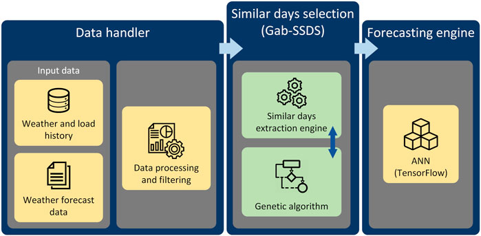
FIGURE 1. The STLF infrastructure.

The Gab-SSDS method can act independently regardless of the chosen forecasting engine. As a result, similar days selection module is entirely autonomous, decoupled from other modules, and fully reusable. In addition, the Gab-SSDS method can be used as an input for the arbitrary load forecast method, either based on the Artificial Neural network or other methodologies, like Linear Regression, Support Vector Machine (SVM), etc. In this particular case, to perform the experiments and evaluate the proposed method, an engine based on the artificial neural network has been used (TensorFlow library) (Abadi et al., 2016).

The overall flowchart of load forecasting process supported with the proposed similar day calculation method is presented in (Figure 2). Gab-SSDS module receives an initial set of days from the Data Handler module. Gab-SSDS uses weight coefficients optimised by the genetic algorithm in a separate process. The output of the Gab-SSDS module is a set of similar days, which is used to produce the input rows to the forecasting engine. Hyper-parameters for ANN training are once optimised, also by genetic algorithm. The output of ANN prediction is the planned load for the forecasting period.

FIGURE 2

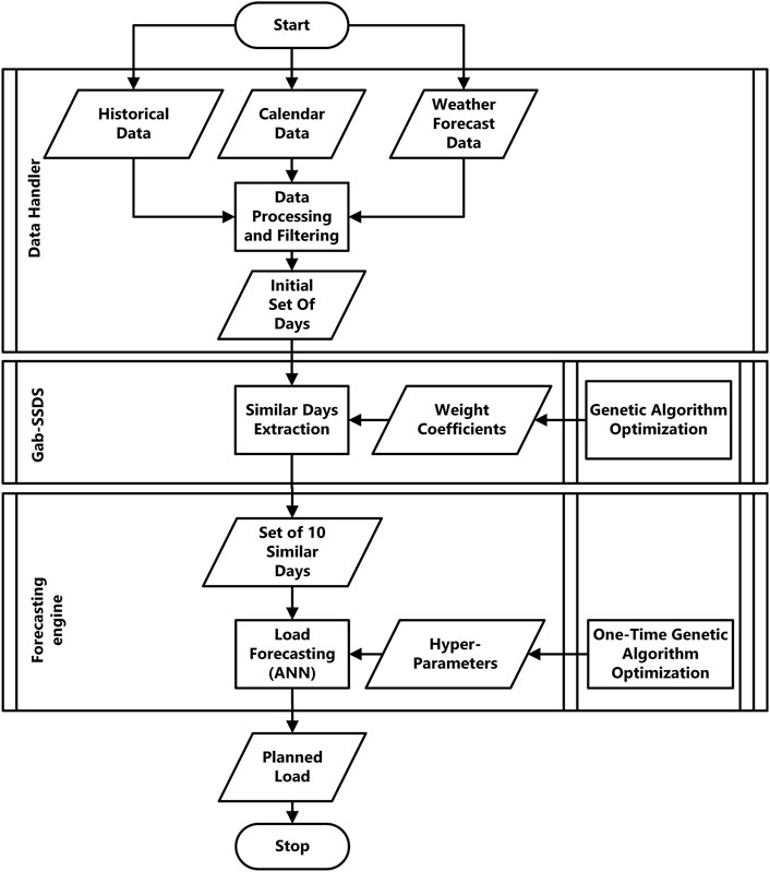
FIGURE 2. Load forecasting method flow chart.

Details about the Gab-SSDS method, used input data, data processing, and overall forecasting process are presented in the following sections.

3.1 Data Handler

Data handler uses weather forecast data and historical load and weather data as inputs, and implements the initial filter that executes data preparation and pre-processing. The filter includes day selection based on a day of a week and rough temperature similarity–days with an average temperature in a close temperature range, compared with forecasting day. The generated output of this module is an initial set of days.

3.1.1 Input Data

The data model required for the forecasting process collects and stores all data necessary for the successful implementation of the algorithm. This model details:

• Weather forecast–represents the instances of the hourly weather forecast. It contains weather type (e.g., temperature, wind speed, humidity, sky cover, daylight duration, etc), forecast value, and timestamp.

• Load history–represents the instances of realised load per hour through the history.

• Weather history–represents the instances of weather data per hour through the history. It includes weather type, measured value, and measurement time.

The model also keeps track of geographical areas for which forecasting is being made, time intervals for data import, weather types, calendar data and current users responsible for customising and initiating calculations.

3.1.2 Data Processing and Filtering

The purpose of the Data processing and filtering module is to prepare data and to exclude days with utterly inadequate calendar and meteorological characteristics. Since temperature is the most important information of all weather variables, it is used most commonly in the regression approach. However, with the use of additional factors, better results should be obtained (Park et al., 1991). In this respect, only days with the same day of the week and temperature range as of the forecasting day are selected from the history database. Day types are defined on the basis of the natural classification: \{Monday\}, \{Tuesday, Wednesday, Thursday\}, \{Friday\}, \{Saturday\} and \{Sunday\} (Alexander Bruhns and Deurveilher, 2005). The temperature range is defined as the actual average temperature from historical data, plus/minus 5 degrees comparing to the predicted average temperature of the forecasting day. In this way, days that do not have approximately the same characteristics as the forecast day are excluded from consideration, which increases the algorithm’s performance. Other factors, like hourly temperature, wind, sky cover and load inertia, are further filtered to detect similarity with the forecasting day more precisely.

3.2 Gab-SSDS Method

Choosing the best parameter setting is an essential and challenging task in evolutionary algorithms. The calculation of the dissimilarity coefficient is based on similarity factors and their weight coefficients. Each similarity factor is assigned with the weight coefficient representing a level of influence of similarity factors on calculated coefficients. Values of weight coefficients may have different optimal values depending on different circumstances such as geographic location, electrical network infrastructure or habits of the population. Furthermore, optimal values of weight coefficients can vary by the period of the year. The approach for weight coefficient adjustment proposed in this paper is implemented with a continuous genetic algorithm.

3.2.1 The Similar Days Extraction

As an initial step in the similar days selection phase, the forecast day and past days are evaluated, and a set of similar days is selected from the past based on a level of similarity. The level of similarity for historical days is determined by dissimilarity coefficient. It is calculated for each historical day by the following equation:

$D_c=\frac{{\sum }_{j=1}^{nsf}SF{D}_{j}w{f}_j}{{\sum }_{j=1}^{nsf}w{f}_j},(1)$

where:

nsf–number of similarity factors. The most common similarity factor is temperature, and it can be used as hourly temperature and daily temperature. Other similarity factors are wind, humidity, and other meteorological factors. Similarity factors can also be calendar factors, e.g., daylight duration.

SFD_j–Similarity Factor Difference for jth similarity factor. It is calculated as a difference between similarity factors for history day and forecast day and can represent an absolute difference between daily values (e.g., daily temperatures) or as an average hourly factor deviation between 2 days (e.g., for hourly temperature).

wf_j–Weight coefficient for jth similarity factor. It is an indicator of a relative contribution of the similarity factor in the dissimilarity coefficient. The calculation of useful dissimilarity coefficients depends primarily on these variables.

The lower dissimilarity coefficient indicates a higher similarity between selected days. Once the similarity level has been calculated, the top n most similar days (with the lowest dissimilarity coefficient) are selected.

3.2.2 The Weight Coefficients Tuning With the Genetic Algorithm

A flow of genetic algorithm implementation in Gab-SSDS method implies an iterative execution of similar days extraction phase with different combinations of weight coefficients until the exit criterium is reached. (Figure 3). Optimised values of weight coefficients are stored in the database after successful GA execution.

FIGURE 3

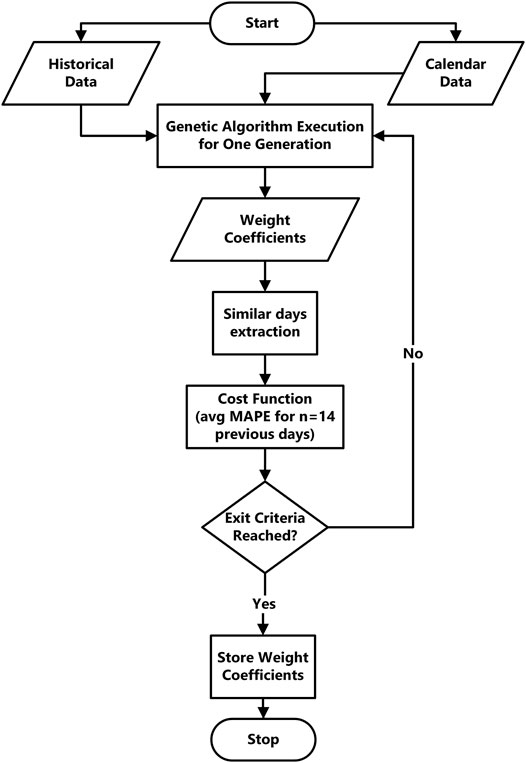
FIGURE 3. Flow chart of GA.

Gab-SSDS uses continuous GA for determining continuous variables - weight coefficients for similarity factors (Figure 4). Variables intended for determination are called genetic variables or genes. In this case, genes represent the weight coefficients of the similarity factors. Genes are arranged in rows called Chromosomes. Every chromosome represents a combination of variable values. In the Gab-SSDS method, the chromosome represents one combination of weight coefficients for the chosen similarity factors.

FIGURE 4

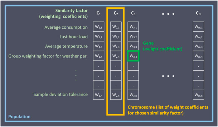
FIGURE 4. Genetic algorithm terminology.

Chromosomes are grouped into population. The population represents the list of chromosomes, or, in this case, the list of possible combinations of weights for chosen similarity factors. In this work, the population consists of 64 chromosomes. The goal is to find the optimal chromosomes, that is, chromosomes with the lowest value of cost function. Chromosomes with higher cost function values are abandoned. Chromosomes with lower cost function value cross over and generate new chromosomes with combined values of genetic variables. This procedure is repeated until defined exit criteria–three iterations without decreasing function cost in resting chromosomes.

The initial population is a random creation of chromosomes consisting of genes–weight coefficients for similarity factors. The variables in the initial population have random values between 0 and 100. As genetic variables represent possible values of weight coefficients, every genetic variable contains the minimal value and maximal value. Chromosomes in the initial population consist of variables with random values between minimal and maximal values.

The Cost Function generates an output of the variable set (chromosome). Every chromosome has assigned the output value of the cost function. Chromosomes are sorted based on their cost values in such a way that chromosomes with lower cost values are better positioned. Thirty-two chromosomes with higher cost values are abandoned, and the remaining 32 chromosomes cross with each other and create new 32 chromosomes. Chromosome pairs are selected by weighted random pairing. The selection probabilities assigned to the chromosomes are inversely proportional to their cost (Tanese, 2004).

The cost function in the presented model is defined as an average Mean Absolute Percentage Error (MAPE) for n days that precede the forecasting day (Chai and Draxler, 2014) in a single-chromosome cost function execution. The number of n days is adjustable, and it depends on the region on which forecasting is executed and mid-term weather stability in that region. In the proposed solution, daily GA is executed for the n = 14 previous days. This period is used for GA optimisation only. It is considered as big enough for finding optimal weight coefficients at the point of the year, but also small enough to prevent time over-consumption of the GA (Shayeghi et al., 2009).

In order to calculate MAPE for 1 day in history, it is necessary to make the load forecast for that day and calculate MAPE between forecasted and observed load. In the real-time execution (outside of the genetic algorithm), the load forecast is performed by ANN as a selected forecasting engine. However, the cost function of every chromosome in the genetic algorithm is based on the arithmetic mean (AM) of load in best ranked similar days (days with minimum dissimilarity coefficients). MAPE is obtained by comparing AM and actual load. Load forecasting in GA cost function is used this way for two reasons:

1) in GA cost function, the goal is not the best possible accuracy of load, but the best possible similarity of days,

2) in this manner, a high-performance saving is made because time-consuming load forecast (e.g., ANN) execution is avoided in GA optimisation.

Day similarity calculation can have more local minimums, and there is a possibility of converging to some of the local minimums. Hence, some chromosomes have to be mutated. The mutation prevents convergence too fast to some of the local minimums before sampling the entire cost surface. In each iteration, six chromosomes mutate in a population. The number of mutated genes in every mutated chromosome is a randomly selected value from one to four.

3.3 Calculation of the Load Forecast

Similar days selection aims to provide input data for the load forecasting process. Even though Gab-SSDS is designed to apply to all forecasting techniques, in this study, it is combined with TensorFlow artificial neural network to investigate its usability and effectiveness.

Artificial Neural Network is a powerful tool for non-linear inputs and prediction problems (Raza et al., 2013). ANN mimics human brains to learn the relationship between certain inputs and outputs from experience (Hong, 2010). The popularity of ANN is based on its ability to model complex relationships that are difficult to identify with traditional techniques (Hippert et al., 2001; Mandal et al., 2006). A typical ANN deployed for STLF is a multi-layer feed-forward ANN, which consists of input, hidden and output layers interconnected by some modifiable weights, represented by the links between the layers. The computational units in each layer are called neurons (Hong, 2010). values of TensorFlow is an open-source artificial intelligence programming system released by Google in 2015 (Abadi et al., 2015). It is used primarily for deep neural networks and machine learning (Zhang et al., 2017). It can efficiently support large-scale training and inference as well as flexible support experimentation and research into new models and system-level optimisations (Jia et al., 2018). TensorFlow includes features like a high degree of flexibility, portability, automatic differential design, and performance optimisation (Qin et al., 2019). STLF refers to a forecasting period of up to 7 days (Gross and Galiana, 1987). The forecasting horizon in the presenting model depends on supplied weather forecast data and cannot extend 7 days.

The proposed forecasting engine is a feed-forward multi-layer neural network model. Days with minimum dissimilarity coefficients, along with their load and weather data, are input to ANN training. Predictor data includes weather data, load inertia, and calendar data, while predicted data is hourly load. ANN predicts future hourly load using weather forecast, load inertia data, and calendar data as predictor parameters. Load inertia data for the forecasting day is realised load in previous days. ANN training and prediction is executed for each hour in the forecasted day. The number of hidden layers and the number of neurons in each hidden layer are obtained through optimisation, along with other hyper-parameters.

The output of ANN prediction is the hourly planned load for the forecast period. Planned load data contains starting and ending time, time resolution, user, geographical area, and a value of the planned load. It represents the output of the system.

3.4 Tuning the Hyper-Parameters

Optimisation of hyper-parameters is another challenge that should be met for the effective use of the ANN. Values of hyper-parameters can be determined manually, looking at training results and predictions using different values of hyper-parameters. However, in this work, hyper-parameters have been determined using a genetic algorithm. Chromosomes are combinations of genes, while each gene represents one value of one specific hyper-parameter. The population is consisted of 64 chromosomes. The cost function for the genetic algorithm is MAPE weighted by execution time. The cost function is obtained by training and prediction of ANN with different values of hyper-parameters. Genetic algorithm optimised hyper-parameters once, and these hyper-parameters were utilised for further forecasting calculations.

Hyper-parameters determined by the genetic algorithm are batch size, number of hidden layers, learning rate, optimiser, activation function, number of neurons in first hidden layers, number of neurons in other hidden layers, optimal input layer, and number of samples. The optimal input layer is the combination of predictors (features). Every possible predictor is a gene with possible values 0 and 1, indicating if the predictor should be used. Determining the optimal number of samples refers to the number of similar days used as input to the neural network.

Genetic algorithm execution was completed after 24 iterations. Figure 5 shows the Pareto frontier diagram (Michel et al., 2019; Mostafa et al., 2020; Izquierdo et al., 2021), with optimal solutions from each iteration. Dominant solutions are the ones that dominate either in terms of accuracy or execution time. The selected solution is marked as the one with the lowest MAPE. However, every dominant solution can be chosen, considering accuracy or execution time preference.

FIGURE 5

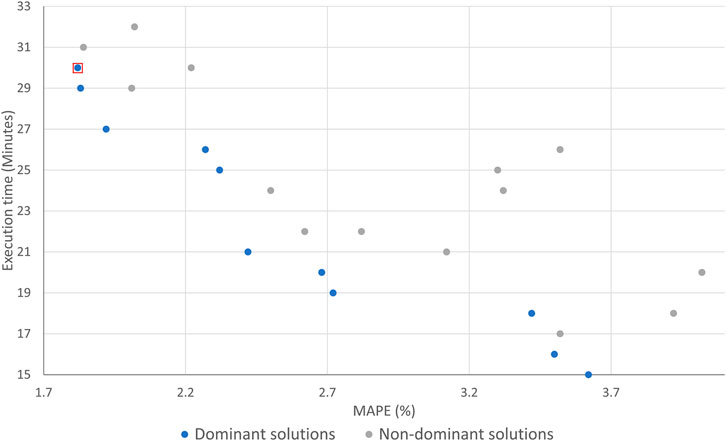
FIGURE 5. Optimal solutions in Pareto diagram.

Table 1 contains value range, step, and final values for each optimised parameter. Figure 6 shows the structure of ANN with optimised layer structure.

TABLE 1

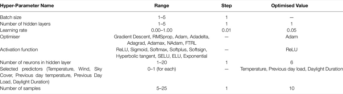
TABLE 1. Optimised ANN hyper-parameters.

FIGURE 6

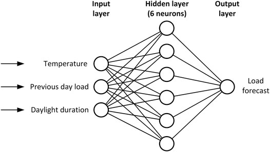
FIGURE 6. Structure of used neural network.

4 The Research Methodology

The goal of this study is to investigate the forecast accuracy, the effectiveness of the proposed method and the possibilities for the whole-year continuous optimisation for similar days selection based on genetic algorithm (Gab-SSDS method). Analysing methods’ strengths and weaknesses could provide us with guidelines to further improve the short-term load forecasting based on the selected similar days. In this section, the used dataset, the approach, the metrics and the measurements used for the data analysis will be described. Such setup is used to perform simulation, the details of which are presented in Section 5.

4.1 Dataset

The study used the electrical load published by Statnett, the system operator of the Norwegian power system¹. This data includes hourly load in transmission for the area of Norway. Historical hourly weather data used in the simulation has been downloaded from the website designed and supported by Raspisaniye Pogodi Ltd.², for the same period and city of Oslo, including temperature, wind speed, sky cover, and humidity. Training and testing data includes a period starting from 1 December 2015, until 30 November 2020.

4.2 The Course of the Experiment

The experiment involves daily short-term load forecasting for 1 day ahead, during 1 year, from 1 December 2019, until 30 November 2020. It includes 365 daily load forecasts. The model is updated with fresh history data and weather forecast data once per day. Every daily load forecast is performed at midnight, and it predicts hourly load on the forecasting day. At the moment when daily forecasting starts, all historical data and weather forecast data for the forecasting day are present.

4.3 Approach

A deductive and quantitative approach is applied in order to answer the proposed research questions. Considering the focus of the study, the authors wanted to understand how the proposed algorithm performs in real-time. The experiment was performed in three phases (Figure 7): 1) development of the algorithm (details presented in Section 3.2), (2) simulation and data collection, and 3) analysis of the results (Section 4.4).

FIGURE 7

FIGURE 7. Phases of the experiment.

In order to investigate the benefits that the proposed method can bring to the load forecasting process, simulation of the load forecast has been executed on the used dataset and with STLF method based on TensorFlow neural network (Abadi et al., 2016) for load forecast. The simulation included the execution of the STLF method using two forecasting approaches (FA1 and FA2):

• FA1: STLF using ANN without Gab-SSDS method. The entire available history of days grouped by day of the week has been used as an input for STLF using TensorFlow neural network.

• FA2: STLF using ANN with Gab-SSDS method. The proposed forecasting method with similar days selection from the entire available history has been used as an input for STLF using TensorFlow neural network. The chosen number of selected similar days in this use case is 10 (as explained in Section 3.4).

The two forecasting approaches have been simulated and applied to the same dataset and time frame. In both cases, forecasting for every day was performed for the period 00:00–23:00 and every hour separately. In each separate daily forecast, historical data is available for the entire period before forecasting. In the FA1 approach, the dataset used for ANN training was a complete data history up to that date, filtered by a day of the week. For a data history of 2 years, every training dataset had a size of up to 104 weeks (2 years multiplied by 52 weeks). Every hour was forecasted separately, and therefore 24 ANN forecasts were executed every day.

In the FA2 approach, data preparation included GA execution and similar days extraction. The genetic algorithm determined the number of 10 similar days as input to ANN training. 24 ANN-based forecasts (with 10 similar days training dataset) were executed every day in the experimental period.

To answer the RQ1 research question and measure the forecast accuracy and, ultimately, effectiveness of the proposed method, the authors compared the forecasted load with the realised load, using two evaluation metrics: Mean absolute percentage error (MAPE) (Khair et al., 2017) and Root Mean Square Percentage Error (RMSPE) (Chai and Draxler, 2014) (described in more details in Section 4.4). The accuracy of the load forecast based on the proposed Gab-SSDS method is determined by comparing the forecasted daily load with realised daily load for the experimental period. More precisely, during simulation, the method generated a load forecast for each day, and these forecast results were compared with the realised load. Besides, the authors compared the forecast results of approaches FA1 and FA2.

In order to answer the RQ2 research question, the authors compared the execution time of ANN forecasting for approaches FA1 and FA2. In both cases, the execution time represents a total time of execution, including both data preparation and forecast execution. Calculated weight coefficients and their average monthly values were analysed to address the RQ3.

4.4 Data Analysis and Evaluation Metrics

The authors introduced several metrics to analyse the results and quantify the forecast accuracy and the effectiveness of the proposed algorithm. Several models are used in the literature to determine which formulations produce more accurate and precise estimations of the variables of interest. Many different statistical methodologies for deviation analysis have been applied in order to evaluate the effectiveness of estimation methods (Willmott and Matsuura, 2005; Chai and Draxler, 2014). The most regularly utilised studies in the model evaluation are the mean absolute percentage error (MAPE) and Root Mean Square Percentage Error (RMSPE) (Willmott and Matsuura, 2005).

Mean Absolute Percentage Error–MAPE represents forecast accuracy of a forecasting method. MAPE is calculated using the absolute error in each period divided by the observed values that are evident for that period. Then, those fixed percentages are averaged. This approach is useful when the size of a prediction variable is significant in evaluating the accuracy of a prediction (Khair et al., 2017). MAPE indicates how high is the error in prediction compared with the real value. MAPE divides each error individually, so it can distort the results as they are highly impacted by high errors during periods with low demand.

$MAPE=\frac{100\%}{n}\sum _{t=1}^n\left|\frac{A_t-F_t}{A_t}\right|(2)$

Calculation of the root-mean-square percentage error–RMSPE involves a sequence of 3 simple steps (Willmott and Matsuura, 2005). Total square error is obtained first as the sum of the individual squared errors; that is, each error influences the total in proportion to its square rather than its magnitude. High hourly errors, as a result, have a relatively greater influence on the total square error than smaller errors do.

$RMSPE=100\cdot \sqrt{\frac{1}{n}\sum _{t=1}^n{\left(\frac{A_t-F_t}{A_t}\right)}^2}(3)$

The pros and cons of the use of both measures have been discussed in numerous papers (Willmott and Matsuura, 2005; Chai and Draxler, 2014). Both deviation metrics were used to exploit the benefits and minimise the drawbacks of these approaches. The RMSPE is more appropriate to represent model performance than the MAPE when the error distribution is expected to be Gaussian (Chai and Draxler, 2014). MAPE protects against outliers, whereas RMSPE provides the assurance to get an unbiased forecast and gives greater importance to the highest errors. While they have both been used to assess model performance for many years, there is no consensus on the most appropriate metric for model errors (Chai and Draxler, 2014). Since both measures are defined differently, they are expected to generate different results. Therefore, a combination of metrics was used in this paper to assess model performance and to provide a complete picture of error distribution (Chai and Draxler, 2014).

5 Simulation Results

This section presents the results of the executed simulation. The simulation was performed following the strategy in five stages. The first stage of the simulation examines the effectiveness of genetic algorithm optimisations. The second stage depicts the weight coefficients tuned by GA. The third stage examines the forecasting accuracy of the proposed load forecast technique using the Gab-SSDS method. In the fourth stage, the effectiveness and overall performance of two load forecasts (with and without the Gab-SSDS method) are compared. In the fifth stage, results are compared with other forecasting methods.

5.1 The Effectiveness of ANN Training

For proving the effectiveness of ANN training, learning curves were tracked. They show the diverging behaviour of in and out-of-sample performance as a function of the number of training iterations for a given number of training examples (Perlich, 2010). They provide insight into the dependence of a learner’s generalisation performance on the training set size (Viering and Loog, 2021).

Learning curves are generated for training and validation datasets. Twenty similar days are selected from the Gab-SSDS filter. This set is divided into two new sets, consisting of 10 randomly selected days. One set is used as the training dataset, and another is used as the validation dataset. The training was tracked for the first hour of the first day of the experiment (1 December 2019).

Figure 8 shows learning curves of training and validation datasets. They show decrements of loss (x-axis) through training iterations (y-axis). The training curve indicates the fitness between the model and the training data, while the validation curve indicates the fitness between the model and new data. Both curves had approximately the same trajectory. Root Mean Square Percentage error between the curves is 12.08%. The learning curves show the high efficiency of ANN training for the selected input data and optimised hyper-parameters.

FIGURE 8

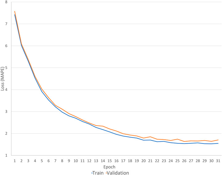
FIGURE 8. ANN learning curves for training and validation datasets.

5.2 The Effectiveness of Genetic Algorithm Optimisation

The primary goal of the optimisation by the genetic algorithm is an adequate selection of similar days used as an input to the forecasting mechanism. The GA cost function is the average daily load that precede the forecasting day. GA optimisation stops when there is no improvement in the average cost function for resting chromosomes in three consecutive iterations. Table 2 shows selected effectiveness parameters of GA used in the Gab-SSDS method: average initial cost function value, average final cost function value, the average convergence rate, the average number of iterations, and the average convergence rate per iteration. The initial cost function value is the cost value of the best individual in the first iteration, and the final cost function value is the cost value of the best individual in the last iteration. The average convergence rate decreases the cost function from the initial to the final cost function value.

TABLE 2

TABLE 2. Effectiveness parameters of GA in Gab-SSDS.

The average convergence rate of 0.38 in average 56.34 iterations (0.007 average convergence rate per iteration) indicates a steady convergence in GA optimisation. However, the more profound analysis of GA optimisation effectiveness is out of this work’s scope.

5.3 Weight Coefficients Tuning

GA optimisation was applied on all days of the testing dataset. Every separate optimisation used its history of days as input to GA. The output of every GA optimisation was a set of weight coefficients of similarity factors for similar days extraction. In this manner, the set of 10 similar days was selected. This set of similar days was used for ANN-based forecasting. During the time, optimised values of the weight coefficient had different values. Table 3 shows the average optimised weight coefficient values of each similarity factor. Five factors with the highest weight coefficients are further analysed.

TABLE 3

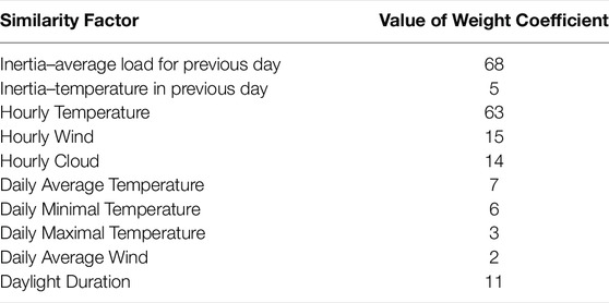
TABLE 3. Tuned weight coefficients of similarity factors.

Table 4 shows average optimised values of weight coefficients per month in the testing dataset for five selected factors (with the most substantial influence).

$D_c=\frac{LoadDif\cdot 68+HTempDif\cdot 61+HCloudDif\cdot 14+HWiDif\cdot 15+DDurDif\cdot 11}{68+61+15+14+11},(4)$

where:

• LoadDif–Average hourly load difference between the day that precedes the similar day and day that precedes the forecasting day,

• HTempDif–Average hourly temperature difference between the similar day and the forecasting day,

• HCloudDif–Average hourly cloud difference between the similar day and the forecasting day,

• HWiDif–Average hourly wind difference between the similar day and the forecasting day,

• DDurDif–Daylight duration difference between the similar day and the forecasting day.

TABLE 4

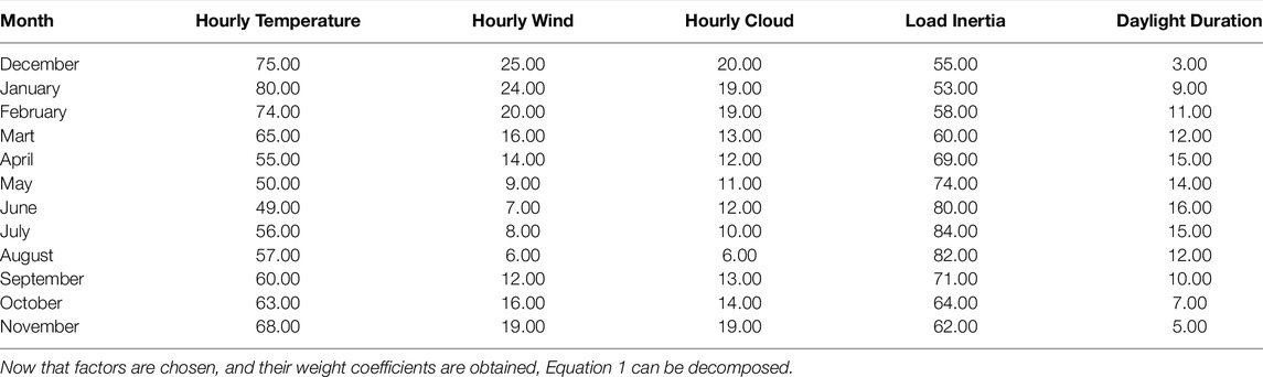
TABLE 4. Average weight coefficients per month.

The dissimilarity coefficient equation is applied to every day previously selected by the data handler.

5.4 Forecast Accuracy

Two error metrics (MAPE and RMSPE) have been used to estimate the forecast accuracy of the FA1 and FA2 methods. The results, shown in Figure 9, are grouped by months. The first columns represent the overall MAPE for FA1 (1.82), the overall MAPE for FA2 and RMSPE for FA2 (2.52). RMSPE for FA1 is shown to depict an influence of outliers. The presented results are significant, as, in the community, all MAPE results smaller than 2% are concerned acceptable (Dong et al., 2017; Hossen et al., 2017; Amber et al., 2018).

FIGURE 9

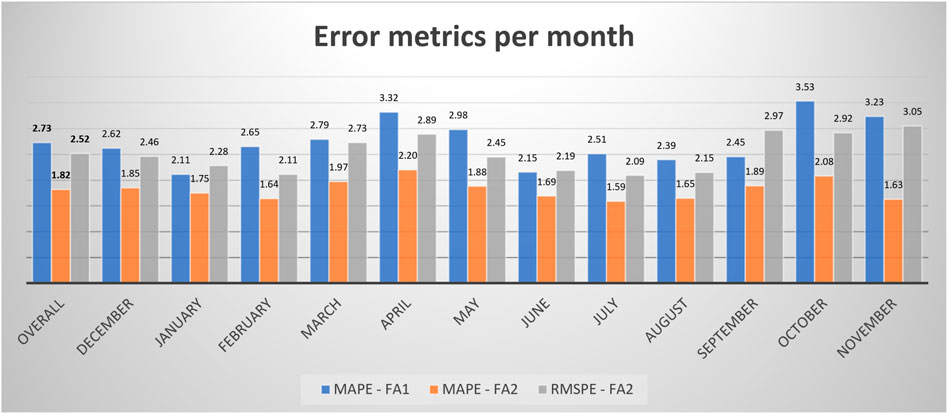
FIGURE 9. Error metrics distribution.

Figure 10 presents the box and whisker plot (Massart and Smeyers-verbeke, 2005) with the distribution of forecast accuracy for the presented algorithm (calculated only with MAPE). It can be noted that the majority of prediction errors fall below 3%, with only seven outliers. Therefore it can be concluded that the presented algorithm proves to be accurate.

FIGURE 10

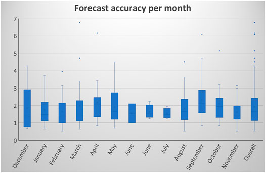
FIGURE 10. Forecast accuracy distribution.

5.5 Comparison of Two Approaches

In order to compare two approaches, FA1 and FA2, their forecast accuracy (effectiveness) and execution times (performance) were measured.

Comparing MAPE for FA1 and FA2 (Figure 9), it is evident that the Gab-SSDS method for similar days selection (approach FA2) outperforms the same algorithm without Gab-SSDS in terms of forecast accuracy (effectiveness). FA2 shows better results in both overall (1.82 with Gab-SSDS vs. 2.73 without Gab-SSDS) and segmented view (for each month in the experimental period). It is noticeable that Gab-SSDS significantly improves the overall forecasting and provides a more accurate forecast.

To compare the performance of the approaches, an analysis of their execution time has been performed for the first forecasting day of the testing data set. Table 5 shows a comparative presentation of execution time for approaches FA1 and FA2. As can be seen, data preparation time is a bit longer for FA2 for the reason that it includes an execution of GA and similar days extraction. On the other hand, data preparation for FA1 is almost instant, as it only includes the selection of days from the history database and weather forecast database. However, forecast execution for FA1 lasts disproportionately longer for the reason that the training data size for FA2 is significantly smaller than for FA1.

TABLE 5

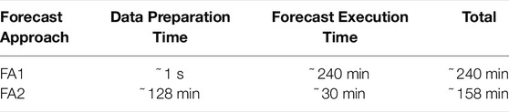
TABLE 5. Execution times for two approaches.

5.6 Comparison With Other Methods

To confirm the effectiveness of Gab-SSDS, the proposed method is also compared with other methods:

1. Hybrid PSO–SVM method for short-term load forecasting (Selakov et al., 2014), which uses Support Vector Machine (SVM), Particle Swarm Optimisation (PSO) for optimisation of SVM parameters, and selection of similar days which adapts to significant temperature variations, and

2. Day similarity metric model for short-term load forecasting supported by PSO and artificial neural network (Janković et al., 2021), which uses Particle Swarm Optimisation for optimal selection of similar days, and ANN as a forecasting engine.

All three methods were applied on the same dataset as Gab-SSDS, and the same testing period: 1 December 2019, until 30 November 2020. The results are present in Table 6.

TABLE 6

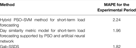
TABLE 6. Comparison Gab-SSDS and other methods.

Obtained results show the more accurate results of Gab-SSDS compared with other methods.

6 Discussion

The presented experiments were designed to address the proposed research questions and to investigate: the forecast accuracy of the Gab-SSDS method (RQ1), increased effectiveness and performance when ANN-based load forecast is combined with Gab-SSDS method (RQ2) and applicability of the method for the weight coefficients optimisation (RQ3).

The analysis of the results gained by the Gab-SSDS method in combination with TensorFlow ANN showed that overall load forecast resulted in accurate results with MAPE values below 2% or slightly above 2% for all months (Figure 9) and with significant forecast accuracy distribution (Figure 10). These results, even though significantly accurate, only provide proof of the applicability of the method as input for the ANN forecast method (affirmative answer for the RQ1). However, to prove that the Gab-SSDS method increased the effectiveness and performance of the overall approach, additional experiments have been executed. Parallel execution of load forecast based on TensorFlow ANN, with and without support of GAB-SSDS method for similar days selection have been simulated.

Two forecasting approaches were named FA1 and FA2, and they represented the same forecasting approach, with and without the support of Gab-SSDS method, respectively. As presented in Section 5 the approach FA2, supported by the proposed method, outperforms the FA1 approach, in terms of forecast accuracy (effectiveness–Figure 9) and overall performance (Table 5). FA1 uses the entire dataset, and therefore it does not spend time for data preparation. However, the large dataset increases the execution time of the ANN forecast. In addition, FA2 spends time for data preparation (including GA optimisation). However, the smaller dataset saves time for the ANN forecast execution, and FA2 spends less total time than FA1. These results confirm a positive answer to RQ2.

As can be noted in Table 3, similarity factors with the highest values of weight coefficients are load in the previous day–Inertia, and hourly temperature. However, weight coefficients for hourly temperature decrease from January to June, have stable values during the summer and increase from September to November. The weight coefficient for load inertia has the opposite behaviour in the same interval (Table 4). Weight coefficients for hourly wind and hourly cloud have a trend similar to hourly temperature. The assumption of the reason for observed trends is the fact that consumers in Norway spend more electricity for heating when temperature decreases, and therefore weight coefficients of weather factors have higher values in these periods. On the other hand, when temperatures are higher, weight coefficients for weather factors decrease, and the primary factor becomes load inertia. Considering observed trends, the authors give an affirmative answer to RQ3: GA can optimise weight coefficients of influential factors of similar days extraction during different periods of the year. Simulation results demonstrate that the implemented method is suitable for short-term load forecasting as it provides accurate forecast and high performance.

The comparison of the developed method with other methods that use meta-heuristic optimisation and non-linear forecasting engines indicated the visible advantage of the Gab-SSDS method in terms of the forecasting results precision. Overall experimental results suggest clear benefits the proposed method can offer to the short term load forecast.

6.1 Limitations of the Study

In order to evaluate the proposed similar days selection method (Gab-SSDS), ANN has been used as the forecasting engine. However, other forecast methods could have been used, such as linear regression, support vector machine or more advanced machine learning techniques. The fact that only ANN has been tested potentially limits the value of results, and additional studies are required to evaluate the suitability of the similar days selection method in combination with other load forecasting engines.

Another limitation of the study is that the load forecast was only tested for 24 h ahead. The influence of similarity factors may have different values for more extended forecasting periods. Therefore GA can be adapted accordingly to optimise weight coefficients for similarity factors depending on the forecasting periods.

7 Conclusion

In the field of short term load forecasting, accurate predictions are made based on a vast amount of correct and accurate historical weather and load data. However, wrong data (outlines, missing or data exceptional) or misleading data (low relevance) are unavoidable and can interfere with the forecasting process and thus reduce the forecast accuracy. Therefore, in order to establish accurate forecasts, the filtering of correct and relevant data is essential to provide relevant input for load forecast algorithms. This paper presented the method for similar data selection that generates a list of days from the past that represents the appropriate historical data as input for a short term load forecast. The implemented Gab-SSDS method is based on the integration of genetic algorithm and similar days selection method. The common use of the genetic algorithm in the load forecast is optimising the parameters of the forecasting engine. Besides optimisation of forecasting engine, the proposed solution uses the genetic algorithm to enhance the forecasting methods by providing relevant input data by tuning the parameters used for similar days selection. Even though the methods can be used as an input method for different load forecasting methods, in order to prove its effectiveness and evaluate its performance, it has been tested with a commonly used TensorFlow artificial neural network. With considerable caution and the respective contextual limitations, we want to report positive findings for the feasibility and potential of using this similar days selection method (Gab-SSDS) for short term load forecasting.

For future work, as an extension of the proposed method, the authors have an intention to further explore the possibilities for the integration of the proposed method in other STLF techniques. Therefore, the series of experiments and simulations will be performed on other load forecasting approaches based on ANN and other regression models–SVM and linear regression.

Data Availability Statement

The raw data supporting the conclusions of this article will be made available by the authors, without undue reservation.

Author Contributions

ZJ developed the algorithm and performed the experiments. ZJ and BV worked on the experiments’ design, data analysis, and writing of the paper. AS and LB worked on the analysis and improvement of the paper.

Funding

This work was supported under the ERA-Net Smart Grids Plus scheme Grant number 89029 and funded through the Research Council of Norway Grant number 295750 with the project title “Multi-layer aggregator solutions to facilitate optimum demand response and grid flexibility.”

Conflict of Interest

The authors declare that the research was conducted in the absence of any commercial or financial relationships that could be construed as a potential conflict of interest.

Publisher’s Note

All claims expressed in this article are solely those of the authors and do not necessarily represent those of their affiliated organizations, or those of the publisher, the editors and the reviewers. Any product that may be evaluated in this article, or claim that may be made by its manufacturer, is not guaranteed or endorsed by the publisher.

Footnotes

¹Statnett the system operator of the Norwegian power system Website.

²Raspisaniye Pogodi Ltd. Website.

References

Abadi, M., Agarwal, A., Barham, P., Brevdo, E., Chen, Z., Citro, C., et al. (2015). Tensorflow : Large-Scale Machine Learning on Heterogeneous Distributed Systems.

Google Scholar

Abadi, M., Barham, P., Chen, J., Chen, Z., Davis, A., Dean, J., et al. (2016). “Tensorflow: A System for Large-Scale Machine Learning,” in 12th \{USENIX\} Symposium on Operating Systems Design and Implementation \{OSDI\} 16, 265–283.

Google Scholar

Alexander Bruhns, J.-S. R., and Deurveilher, G. (2005). A Non-linear Regression Model for Mid-term Load Forecasting and Improvements in Seasonality. Liège, Belgium: Citeseer.

Google Scholar

Amber, K. P., Ahmad, R., Aslam, M. W., Kousar, A., Usman, M., and Khan, M. S. (2018). Intelligent Techniques for Forecasting Electricity Consumption of Buildings. Energy 157, 886–893. doi:10.1016/j.energy.2018.05.155

CrossRef Full Text | Google Scholar

Baliyan, A., Gaurav, K., and Mishra, S. K. (2015). A Review of Short Term Load Forecasting Using Artificial Neural Network Models. Proced. Comp. Sci. 48, 121–125. doi:10.1016/j.procs.2015.04.160

CrossRef Full Text | Google Scholar

Barman, M., Dev Choudhury, N. B., and Sutradhar, S. (2018). A Regional Hybrid goa-svm Model Based on Similar Day Approach for Short-Term Load Forecasting in assam, india. Energy 145, 710–720. doi:10.1016/j.energy.2017.12.156

CrossRef Full Text | Google Scholar

Berntzen, L., Meng, Q., Vesin, B., Johannessen, M. R., Brekke, T., and Laur, I. (2021). “Blockchain for Smart Grid Flexibility-Handling Settlements between the Aggregator and Prosumers.,” in International Conference on Digital Society and eGovernments (ICDS). (Nice, France: IARIA).

Google Scholar

Bouktif, S., Fiaz, A., Ouni, A., and Serhani, M. (2018). Optimal Deep Learning LSTM Model for Electric Load Forecasting Using Feature Selection and Genetic Algorithm: Comparison with Machine Learning Approaches †. Energies 11, 1636. doi:10.3390/en11071636

CrossRef Full Text | Google Scholar

Campillo, J., Wallin, F., Torstensson, D., and Vassileva, I. (2012). “Energy Demand Model Design for Forecasting Electricity Consumption and Simulating Demand Response Scenarios in sweden,” in 4th International Conference in Applied Energy 2012 (Suzhou, China).

Google Scholar

Çevik, H. H., and Çunkaş, M. (2015). Short-term Load Forecasting Using Fuzzy Logic and Anfis. Neural Comput. Appl. 26, 1355. doi:10.1007/s00521-014-1809-4

CrossRef Full Text | Google Scholar

Chai, T., and Draxler, R. R. (2014). Root Mean Square Error (RMSE) or Mean Absolute Error (MAE)? - Arguments against Avoiding RMSE in the Literature. Geosci. Model. Dev. 7, 1247–1250. doi:10.5194/gmd-7-1247-2014

CrossRef Full Text | Google Scholar

Chen, L. G., Chiang, H. D., Dong, N., and Liu, R. P. (2016). Group‐based Chaos Genetic Algorithm and Non‐linear Ensemble of Neural Networks for Short‐term Load Forecasting. IET Generation, Transm. Distribution 10, 1440–1447. doi:10.1049/iet-gtd.2015.1068

CrossRef Full Text | Google Scholar

Chen, Y., Luh, P. B., Guan, C., Zhao, Y., Michel, L. D., Coolbeth, M. A., et al. (2009). Short-term Load Forecasting: Similar Day-Based Wavelet Neural Networks. IEEE Trans. Power Syst. 25, 322.

Google Scholar

Chiang, H.-D., and Reddy, C. K. (2007). Trust-tech Based Neural Network Training. in Neural Networks, 2007. IJCNN 2007. International Joint Conference onIEEE, 90–95. doi:10.1109/ijcnn.2007.4370936

CrossRef Full Text | Google Scholar

Defilippo, S. B., Neto, G. G., and Hippert, H. S. (2015). “Short-term Load Forecasting by Artificial Neural Networks Specified by Genetic Algorithms–A Simulation Study over a Brazilian Dataset,” in XIII Simposio Argentino de Investigación Operativa (SIO)-JAIIO 44 (Rosario).

Google Scholar

Dong, X., Qian, L., and Huang, L. (2017). Short-term Load Forecasting in Smart Grid: A Combined Cnn and K-Means Clustering Approach (BigComp) (IEEE).” inIEEE International Conference on Big Data and Smart Computing, 119–125. doi:10.1109/bigcomp.2017.7881726

CrossRef Full Text | Google Scholar

Eapen, R. R., and Simon, S. P. (2019). Performance Analysis of Combined Similar Day and Day Ahead Short Term Electrical Load Forecasting Using Sequential Hybrid Neural Networks. IETE J. Res. 65, 216–226. doi:10.1080/03772063.2017.1417749

CrossRef Full Text | Google Scholar

El Desouky, A. A., Aggarwal, R., Elkateb, M. M., and Li, F. (2001). Advanced Hybrid Genetic Algorithm for Short-Term Generation Scheduling. IEE Proc. Gener. Transm. Distrib. 148, 511–517. doi:10.1049/ip-gtd:20010642

CrossRef Full Text | Google Scholar

Ghayekhloo, M., Menhaj, M. B., and Ghofrani, M. (2015). A Hybrid Short-Term Load Forecasting with a New Data Preprocessing Framework. Electric Power Syst. Res. 119, 138–148. doi:10.1016/j.epsr.2014.09.002

CrossRef Full Text | Google Scholar

Ghofrani, M., Ghayekhloo, M., Arabali, A., and Ghayekhloo, A. (2015). A Hybrid Short-Term Load Forecasting with a New Input Selection Framework. Energy 81, 777–786. doi:10.1016/j.energy.2015.01.028

CrossRef Full Text | Google Scholar

Gross, G., and Galiana, F. D. (1987). Short-term Load Forecasting. Proc. IEEE 75, 1558–1573. doi:10.1109/proc.1987.13927

CrossRef Full Text | Google Scholar

Hahn, H., Meyer-Nieberg, S., and Pickl, S. (2009). Electric Load Forecasting Methods: Tools for Decision Making. Eur. J. Oper. Res. 199, 902–907. doi:10.1016/j.ejor.2009.01.062

CrossRef Full Text | Google Scholar

Heng, E. T., Srinivasan, D., and Liew, A. (1998). Short Term Load Forecasting Using Genetic Algorithm and Neural networksEnergy Management and Power Delivery. Proc. EMPD’98. 1998 Int. Conf. (Ieee) 2, 576.

Google Scholar

Hertel, L., Collado, J., Sadowski, P., Ott, J., and Baldi, P. (2020). Sherpa: Robust Hyperparameter Optimization for Machine Learning. SoftwareX 12, 100591. doi:10.1016/j.softx.2020.100591

CrossRef Full Text | Google Scholar

Hippert, H. S., Pedreira, C. E., and Souza, R. C. (2001). Neural Networks for Short-Term Load Forecasting: A Review and Evaluation. IEEE Trans. Power Syst. 16, 44–55. doi:10.1109/59.910780

CrossRef Full Text | Google Scholar

Hong, T. (2010). Short Term Electric Load Forecasting (Doctoral Dissertation). Raleigh, North Carolina: North Carolina State University.

Google Scholar

Hong, W.-C., Dong, Y., Zhang, W. Y., Chen, L.-Y., and K. Panigrahi, B. (2013). Cyclic Electric Load Forecasting by Seasonal Svr with Chaotic Genetic Algorithm. Int. J. Electr. Power Energ. Syst. 44, 604–614. doi:10.1016/j.ijepes.2012.08.010

CrossRef Full Text | Google Scholar

Hossen, T., Plathottam, S. J., Angamuthu, R. K., Ranganathan, P., and Salehfar, H. (2017). Short-term Load Forecasting Using Deep Neural Networks (Dnn). North American Power Symposium (NAPS) (IEEE). doi:10.1109/naps.2017.8107271

CrossRef Full Text | Google Scholar

Izquierdo, S., Guerrero-Viu, J., Hauns, S., Miotto, G., Schrodi, S., Biedenkapp, A., et al. (2021). “Bag of Baselines for Multi-Objective Joint Neural Architecture Search and Hyperparameter Optimization,” in 8th ICML Workshop on Automated Machine Learning (AutoML).

Google Scholar

Jalali, S. M. J., Ahmadian, S., Khosravi, A., Shafie-khah, M., Nahavandi, S., and Catalao, J. P. S. (2021). A Novel Evolutionary-Based Deep Convolutional Neural Network Model for Intelligent Load Forecasting. IEEE Trans. Ind. Inf. 17, 8243–8253. doi:10.1109/tii.2021.3065718

CrossRef Full Text | Google Scholar

Janković, Z., Selakov, A., Bekut, D., and Djordjević, M. (2021). Day Similarity Metric Model for Short-Term Load Forecasting Supported by Pso and Artificial Neural Network. Electr. Eng. 103, 2973.

Google Scholar

Jawad, M., Ali, S. M., Khan, B., Mehmood, C. A., and Farid, U., (2018). Genetic Algorithm-Based Non-linear Auto-Regressive with Exogenous Inputs Neural Network Short-Term and Medium-Term Uncertainty Modelling and Prediction for Electrical Load and Wind Speed. J. Eng. 2018, 721. doi:10.1049/joe.2017.0873

CrossRef Full Text | Google Scholar

Jia, C., Liu, J., Jin, X., Lin, H., An, H., Han, W., et al. (2018). Improving the Performance of Distributed Tensorflow with Rdma. Int. J. Parallel Programming 46, 674–685. doi:10.1007/s10766-017-0520-3

CrossRef Full Text | Google Scholar

Karimi, M., Karami, H., Gholami, M., Khatibzadehazad, H., and Moslemi, N. (2018). Priority index Considering Temperature and Date Proximity for Selection of Similar Days in Knowledge-Based Short Term Load Forecasting Method. Energy 144, 928–940. doi:10.1016/j.energy.2017.12.083

CrossRef Full Text | Google Scholar

Kavousi-Fard, A., Samet, H., and Marzbani, F. (2014). A New Hybrid Modified Firefly Algorithm and Support Vector Regression Model for Accurate Short Term Load Forecasting. Expert Syst. Appl. 41, 6047–6056. doi:10.1016/j.eswa.2014.03.053

CrossRef Full Text | Google Scholar

Khair, U., Fahmi, H., Al Hakim, S., and Rahim, R. (2017). Forecasting Error Calculation with Mean Absolute Deviation and Mean Absolute Percentage Error. J. Phys. Conf. Ser., 930. doi:10.1088/1742-6596/930/1/012002

CrossRef Full Text | Google Scholar

Khwaja, A., Naeem, M., Anpalagan, A., Venetsanopoulos, A., and Venkatesh, B. (2015). Improved Short-Term Load Forecasting Using Bagged Neural Networks. Electric Power Syst. Res. 125, 109–115. doi:10.1016/j.epsr.2015.03.027

CrossRef Full Text | Google Scholar

Kouhi, S., Keynia, F., and Ravadanegh, S. N. (2014). A New Short-Term Load Forecast Method Based on Neuro-Evolutionary Algorithm and Chaotic Feature Selection. Int. J. Electr. Power Energ. Syst. 62, 862–867. doi:10.1016/j.ijepes.2014.05.036

CrossRef Full Text | Google Scholar

Kyriakides, E., and Polycarpou, M. (2007). “Short Term Electric Load Forecasting: A Tutorial,” in Trends in Neural Computation (Springer), 391–418.

Google Scholar

Li, S., Goel, L., and Wang, P. (2016). An Ensemble Approach for Short-Term Load Forecasting by Extreme Learning Machine. Appl. Energ. 170, 22–29. doi:10.1016/j.apenergy.2016.02.114

CrossRef Full Text | Google Scholar

Liao, G.-C., and Tsao, T.-P. (2006). Application of a Fuzzy Neural Network Combined with a Chaos Genetic Algorithm and Simulated Annealing to Short-Term Load Forecasting. IEEE Trans. Evol. Comput. 10, 330–340. doi:10.1109/tevc.2005.857075

CrossRef Full Text | Google Scholar

Lipo Wang, G. S. (2010). Optimal Location Management in mobile Computing with Hybrid Genetic Algorithm and Particle Swarm Optimization (ga-pso). Athens, Greece: 17th IEEE International Conference on Electronics, Circuits and Systems.

Google Scholar

Liu, A., Li, J., Che, Y., Qian, B., Zhou, M,, and Li, F. (2021). Short-term power load forecasting via recurrent neural network with similar day selection.” in IEEE International Conference on Data Science and Computer Application (ICDSCA) (IEEE).doi:10.1109/icdsca53499.2021.9650231

CrossRef Full Text | Google Scholar

Mandal, P., Senjyu, T., Urasaki, N., and Funabashi, T. (2006). A Neural Network Based Several-Hour-Ahead Electric Load Forecasting Using Similar Days Approach. Int. J. Electr. Power Energ. Syst. 28, 367–373. doi:10.1016/j.ijepes.2005.12.007

CrossRef Full Text | Google Scholar

Massart, D. L., Smeyers-verbeke, A. J., et al. (2005). Practical Data Handling Visual Presentation of Data by Means of Box Plots. Chester, UK: LC-GC Europe.

Google Scholar

Michel, G., Alaoui, M. A., Lebois, A., Feriani, A., and Felhi, M. (2019). DVOLVER: Efficient Pareto-Optimal Neural Network Architecture Search.

Google Scholar

Minerva, T., and Paterlini, S. (2002). “Evolutionary Approaches for Statistical modellingEvolutionary Computation,” in Proc. 2002 Congress (Ieee), Honolulu, HI. (Honolulu, HI: Proceedings of the 2002 Congress on Evolutionary Computation. CEC'02) 2, 022023.

Google Scholar

Mostafa, S. S., Mendonça, F., Ravelo-Garcia, A. G., Gabriel Juliá-Serdá, G., and Morgado-Dias, F. (2020). Multi-objective Hyperparameter Optimization of Convolutional Neural Network for Obstructive Sleep Apnea Detection. IEEE Access 8, 129586–129599. doi:10.1109/ACCESS.2020.3009149

CrossRef Full Text | Google Scholar

Park, D., El-Sharkawi, M., Marks, R., Atlas, L., and Damborg, M. (1991). Electric Load Forecasting Using an Artificial Neural Network. IEEE Trans. Power Syst. 6, 442–449. doi:10.1109/59.76685

CrossRef Full Text | Google Scholar

Perlich, C. (2010). Learning Curves in Machine Learning. Boston, MA: Springer US, 577–580. doi:10.1007/978-0-387-30164-8_452

CrossRef Full Text | Google Scholar

Phyo, P. P., and Jeenanunta, C. (2021). Daily Load Forecasting Based on a Combination of Classification and Regression Tree and Deep Belief Network. IEEE Access 9, 152226–152242. doi:10.1109/access.2021.3127211

CrossRef Full Text | Google Scholar

Prado, F., Minutolo, M. C., and Kristjanpoller, W. (2020). Forecasting Based on an Ensemble Autoregressive Moving Average-Adaptive Neuro-Fuzzy Inference System–Neural Network-Genetic Algorithm Framework. Energy 197, 117159. doi:10.1016/j.energy.2020.117159

CrossRef Full Text | Google Scholar

Qin, J., Liang, J., Chen, T., Lei, X., and Kang, A. (2019). Simulating and Predicting of Hydrological Time Series Based on Tensorflow Deep Learning. Polish J. Environ. Stud. 28. doi:10.15244/pjoes/81557

CrossRef Full Text | Google Scholar

Raza, M. Q., Baharudin, Z., Islam, B., Zakariya, M., and Khir, M. M. (2013). Neural Network Based Stlf Model to Study the Seasonal Impact of Weather and Exogenous Variables. Res. J. Appl. Sci. Eng. Techn. 6, 3729–3735. doi:10.19026/rjaset.6.3583

CrossRef Full Text | Google Scholar

Santra, A. S., and Lin, J.-L. (2019). Integrating Long Short-Term Memory and Genetic Algorithm for Short-Term Load Forecasting. Energies 12, 2040. doi:10.3390/en12112040

CrossRef Full Text | Google Scholar

Selakov, A., Cvijetinović, D., Milović, L., Mellon, S., and Bekut, D. (2014). Hybrid Pso–Svm Method for Short-Term Load Forecasting during Periods with Significant Temperature Variations in City of burbank. Appl. Soft Comput. 16, 80–88. doi:10.1016/j.asoc.2013.12.001

CrossRef Full Text | Google Scholar

Shayeghi, H., Shayanfar, H., and Azimi, G. (2009). Stlf Based on Optimized Neural Network Using Pso. Int. J. Electr. Comp. Eng. 4, 1190–1199.

Google Scholar

Simon, D. (2008). Biogeography-based Optimization, 702–713. doi:10.1109/tevc.2008.919004

CrossRef Full Text | Google Scholar

Srivastava, A., Pandey, A. S., and Singh, D. (2016). Notice of Violation of Ieee Publication Principles: Short-Term Load Forecasting Methods: A reviewICETEESES) (IEEE). International Conference on Emerging Trends in Electrical Electronics & Sustainable Energy Systems, 130–138. doi:10.1109/iceteeses.2016.7581373

CrossRef Full Text | Google Scholar

Sun, W., and Zhang, C. (2018). A Hybrid Ba-Elm Model Based on Factor Analysis and Similar-Day Approach for Short-Term Load Forecasting. Energies 11, 1282. doi:10.3390/en11051282

CrossRef Full Text | Google Scholar

Tanese, R. (2004). Practical Genetic Algorithms. Hoboken, NJ: John Wiley & Sons, Inc.

Google Scholar

Taylor, J. W., McSharry, P. E., et al. (2007). Short-term Load Forecasting Methods: An Evaluation Based on European Data. IEEE Trans. Power Syst. 22, 2213–2219. doi:10.1109/tpwrs.2007.907583

CrossRef Full Text | Google Scholar

Taylor, J. W. (2012). Short-term Load Forecasting with Exponentially Weighted Methods. IEEE Trans. Power Syst. 27, 458–464. doi:10.1109/tpwrs.2011.2161780

CrossRef Full Text | Google Scholar

Viering, T. J., and Loog, M. (2021). The Shape of Learning Curves: A Review.

Google Scholar

Wang, B., and Chiang, H.-D. (2011). Elite: Ensemble of Optimal Input-Pruned Neural Networks Using Trust-Tech. IEEE Trans. Neural networks 22, 96–109. doi:10.1109/tnn.2010.2087354

PubMed Abstract | CrossRef Full Text | Google Scholar

Willmott, C. J., and Matsuura, K. (2005). Advantages of the Mean Absolute Error (Mae) over the Root Mean Square Error (Rmse) in Assessing Average Model Performance. Clim. Res. 30, 79–82. doi:10.3354/cr030079

CrossRef Full Text | Google Scholar

Yu, F., and Xu, X. (2014). A Short-Term Load Forecasting Model of Natural Gas Based on Optimized Genetic Algorithm and Improved Bp Neural Network. Appl. Energ. 134, 102–113. doi:10.1016/j.apenergy.2014.07.104

CrossRef Full Text | Google Scholar

Zhang, M., Xu, H., Wang, X., Zhou, M., and Hong, S. (2017). Application of Google Tensorflow Machine Learning Framework. Microcomputer Its Appl. 36, 58. doi:10.1007/978-981-32-9698-5

CrossRef Full Text | Google Scholar

Zhang, R., Zhang, C., and Yu, M. (2021). A Similar Day Based Short Term Load Forecasting Method Using Wavelet Transform and Lstm. IEEJ Trans. Electr. Electron. Eng. doi:10.1002/tee.23536

CrossRef Full Text | Google Scholar