Regional Ultra-Short-Term Wind Power Combination Prediction Method Based on Fluctuant/Smooth Components Division

When multiple scattered wind farms are connected to the power grid, the meteorological and geographic information data used for power prediction of a single wind farm are not suitable for the regional wind power prediction of the dispatching department. Therefore, based on the regional wind power historical data, this study proposes a combined prediction method according to data decomposition. Firstly, the original sequence processed by the extension methods is decomposed into several regular components by Complete Ensemble Empirical Mode Decomposition with Adaptive Noise (CEEMDAN). All the components are classified into two categories: fluctuant components and smooth components. Then, according to the characteristics of different data, the long short-term memory (LSTM) network and autoregressive integrated moving average (ARIMA) model are used to model the fluctuant components and the smooth components, respectively, and obtain the predicted values of each component. Finally, the predicted data of all components are accumulated, which is the final predicted result of the regional ultra-short-term wind power. The feasibility and accuracy of this method are verified by the comparative analysis.

Introduction

With the vigorous development of wind resources in China, multiple wind farms are connected to the provincial and regional power grid at the same time. Different wind farms are far away and have dispersion characteristics (Gan et al., 2016). In order to face the impact of cluster grid connection on the power system and the power market, it is necessary to predict the regional wind power when making decisions such as operating plans and market transactions (Zalzar et al., 2020). In recent years, regional wind power prediction has become a key technology to improve the operation level of large-scale wind power integration into a power system (Wang et al., 2021). The traditional regional wind power prediction is to accumulate the power prediction results of sub-wind farms or divided small-region wind farms (Lobo and Sanchez, 2012). However, error may occur in the wind power prediction for each wind farm, and it is difficult to consider the dispersion characteristics of prediction error in accumulation (Wang C et al., 2017). In addition, the weather forecasts and geographical features used in the power prediction of each wind farm are different from each other. They are no longer applicable to regional wind power prediction. Therefore, the dispatching department can use the stored regional historical wind power data to complete the forecast, which avoids the accumulation process and does not rely on individual wind farms.

With the rapid development of the smart grid, environmental sensors, and related technologies, artificial intelligence methods have been gradually applied in ultra-short-term wind power prediction. Compared with the traditional support vector regression (SVR) and backpropagation (BP) algorithms, recurrent neural network (RNN) is good at processing time series data. In response to the problem of gradient disappearance or gradient explosion about RNN, the input gate, the output gate, and the forget gate have been introduced in the long short-term memory network (Hochreiter and Schmidhuber, 1997), which can fully reflect the long-term historical information in time series data and showing better performance. Xu et al. (2021) showed that, by combining a similar day with an LSTM network, the ultra-short-term wind power prediction method had been proposed to improve the prediction accuracy. Wu et al. (2021) proposed a spatiotemporal correlation model for the ultra-short-term wind power prediction based on CNN-LSTM. By constructing the error following the forget gate-based LSTM model, the ultra-short-term wind power prediction has been achieved with less prediction error (Zhang et al., 2020). In order to improve the accuracy and reduce the training time, a multilayer bidirectional gated recurrent unit (GRU) is constructed (Chen et al., 2021). However, meteorological data have been used in the abovementioned works, which are not suitable for the regional ultra-short-term wind power prediction. Machine learning methods continue to learn the mapping relationship between input data and output data through training a large number of data samples (Elsaraiti and Merabet, 2021), providing improvement for power prediction only based on historical data. In order to further explore the variation law of wind power data with time and improve the prediction accuracy of training models, many scholars choose wavelet decomposition, Empirical Mode Decomposition (EMD) (Huang et al., 1998), Ensemble Empirical Mode Decomposition (EEMD) (Wu and Huang, 2011), and other methods to decompose the historical data into several regular subsequences (Safari et al., 2017). These methods integrated with the machine learning method can build a combination model. Using the discrete wavelet transform to decompose the non-stationary wind power time series, the obtained components have more stationarity, which is easier to predict (Liu et al., 2019). Similarly, three-stage wavelet decomposition is adopted to smooth the original wind power time series, and the prediction models for each sub-series sample are developed based on the LSTM network. The proposed method overcomes the poor prediction of a single LSTM network for the non-stationary signals (Wang et al., 2019). Compared with the wavelet decomposition technique, the EMD method has more advantages in dealing with nonlinear, non-stationary, and complex time series data. EMD is used to decompose the power load data, and LSTM is used to train the subsequences (Bedi and Toshniwal, 2018). The EEMD-SE technique is used to decompose the original wind power series into a number of subsequences with obvious complexity differences. The forecasting model of each subsequence is created by full-parameters continued fraction (Wang HZ et al., 2017). A novel fault diagnosis method based on EEMD and optimized Elman_AdaBoost is proposed to get better accuracy and real-time processing performance (Fu et al., 2018). In practice, EMD and EEMD have some defects, including mode mixing, large calculation, and difficulties in eliminating auxiliary noise, which limit their application (Mahmoud et al., 2017). Compared with EMD and EEMD, Complete Ensemble Empirical Mode Decomposition with Adaptive Noise (CEEMDAN) (Torres et al., 2011) is more suitable for data decomposition. CEEMDAN is used to decompose wind speed data, and each component is trained based on an improved BP neural network (Qu et al., 2018). The original wind power is decomposed by the CEEMDAN to eliminate the noise of the data. Then, the decomposed wind power is reconstructed into new subsequences (Lu et al., 2021). In addition, to improve the prediction accuracy, the end effect of the intrinsic mode functions (IMFs) obtained by CEEMDAN also needs to be resolved (Huang et al., 2003). There are usually two methods to suppress the end effect. The first is to replace spline interpolation using different interpolation methods, but the degree of suppression is limited. The second is to increase the sequence length by extending the left and right ends of the original sequence, which is proved to be more suitable.

Aiming at the problem of regional wind power prediction with weak regularity, this study proposes a combined prediction method based on modal decomposition and artificial intelligence technology. Through actual analysis, the accuracy of the combined prediction method will be tested by comparison with the actual engineering level and the prediction results of other methods. The main contributions are as follows:

1) CEEMDAN is used to decompose wind power data to solve the problem of mode mixing and difficulties in eliminating auxiliary noise.

2) LSTM, which can reflect the long-term historical information in time series, is used to predict the fluctuant components of wind power.

3) According to the different characteristics of fluctuant and smooth components, LSTM and ARIMA are selected to predict the wind power, respectively, and the prediction results are further combined and optimized.

Processing and Division of Regional Wind Power Historical Data

Before decomposition, the end points of the regional wind power historical data are extended to suppress the end effect. After decomposition, the decomposed subsequences are divided into two categories: fluctuant components and smooth components.

Data Extension Method

The existing extension methods have certain requirements for the original data, making it inapplicable for wind power data because regularity is not obvious. In order to suppress the end effect as much as possible, two different methods are used to deal with the left and right end points, respectively. For the left end points, the data of two pairs of extreme points are extracted forward. In contrast, for the right end points, the data of the two pairs of extreme points are extracted in a symmetrical continuation manner. The extension process is shown in Figure 1.

FIGURE 1

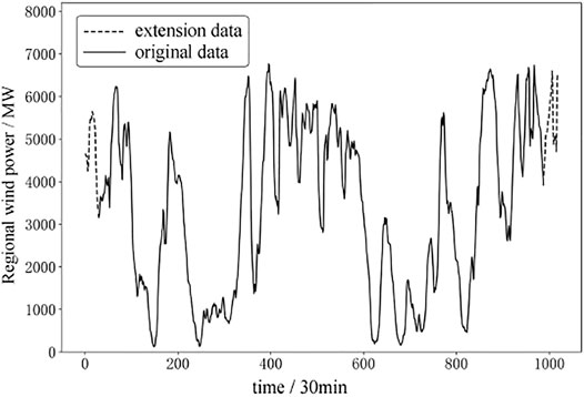
FIGURE 1. Diagram of the data extension process.

Complete Ensemble Empirical Mode Decomposition With Adaptive Noise

CEEMDAN is based on EMD and EEMD. In order to eliminate end effect and reconstruction errors, CEEMDAN replaces the noise data added by EEMD with adaptive white noise. The complete decomposition steps of CEEMDAN are as follows.

1) First, add the I group of normally distributed white noise data w_i(t) to the regional wind power historical data s(t). Construct the I group of new series s_i(t) (i = 1, 2, ··· I). After EMD decomposition is performed to obtain the average value, the first modal component IMF₁(t) is obtained as follows:

${\mathrm{s}}_{\mathrm{i}}\left(t\right)=s\left(t\right)+{\epsilon }_0{W}_i\left(t\right)(1)$

${\mathrm{IMF}}_1\left(t\right)=\frac{1}{I}{\displaystyle \sum _{i=1}^I{\mathrm{IMF}}_1^i\left(t\right)}(2)$

where ε₀ denotes the weight coefficient of Gaussian white noise and IMF₁ⁱ(t) denotes the first IMF after EMD decomposition of s_i(t).

2) Subtracting IMF₁(t) from s(t), the first residual component r₁(t) is obtained as follows:

$r_1\left(t\right)=\mathrm{s}\left(t\right)-{\mathrm{IMF}}_1\left(t\right)(3)$

3) Continue to do EMD decomposition on r₁(t) + ε₁E₁[w_i(t)] to obtain the IMF₂(t) and r₂(t), as shown in Eqs 4, 5:

${\mathrm{IMF}}_2\left(t\right)=\frac{1}{I}{\displaystyle \sum _{i=1}^I{E}_1\{r_1\left(t\right)+{\epsilon }_1{E}_1\left[W_i\left(t\right)\right]\}}(4)$

where E1(·) denotes the first component after EMD decomposition:

$r_2\left(t\right)=r_1\left(t\right)-{\mathrm{IMF}}_2\left(t\right)(5)$

4) Repeat the process of Step 3. Then, IMF_h(t) and r_h(t) can be calculated as follows:

${\mathrm{IMF}}_h\left(t\right)=\frac{1}{I}{\displaystyle \sum _{i=1}^I{E}_1\{r_{h-1}\left(t\right)+{\epsilon }_{h-1}{E}_{h-1}\left[W_i\left(t\right)\right]\}}(6)$

$r_h\left(t\right)=r_{h-1}\left(t\right)-{\mathrm{IMF}}_h\left(t\right)(7)$

5) Until the termination condition is satisfied, h IMF(t)s and a res(t) can be obtained as follows:

$s\left(t\right)={\displaystyle \sum _{i=1}^h{\mathrm{IMF}}_i}\left(t\right)+res\left(t\right).(8)$

Component Judgment Formula

Because the data changes of the latter few IMFs and Res are relatively smooth, modeling these subsequences by fitting can save time. Therefore, a threshold f* is set according to the ratio f of the number of extreme points to the number of original data. When f is greater than f*, these IMFs are judged to be the fluctuant components, and the remaining IMFs and Res are judged to be the smooth components. The extension data are not included when calculating f, and the judgment formula f is as follows:

$f=\frac{M_{\max }+M_{\min }}{N}(9)$

where M_max, M_min, and N denote the number of maximum points, minimum points, and the original data, respectively.

Fluctuant/Smooth Components Prediction Method

After completing the processing and division of regional wind power historical data, the subsequences contained in each component are modeled and predicted, respectively. Because the decomposition results are a number of subsequences with gradually decreasing frequency components, it is more difficult to model the fluctuant components relative to the smooth components.

Prediction Method of Fluctuant Components

Because the fluctuant components contain several IMFs with the highest frequency components, the prediction results of each subsequence in this component will directly affect the final prediction accuracy. RNN is specialized in processing time series data and has a unique memory function for processed data. In order to effectively solve the problem in RNN related to gradient, LSTM adds three control gates on the basis of RNN: the input gate, forget gate, and output gate are added to build LSTM. In addition, it can ensure the model remembers the historical information of an uncertain time. The basic unit model of LSTM is shown in Figure 2.

FIGURE 2

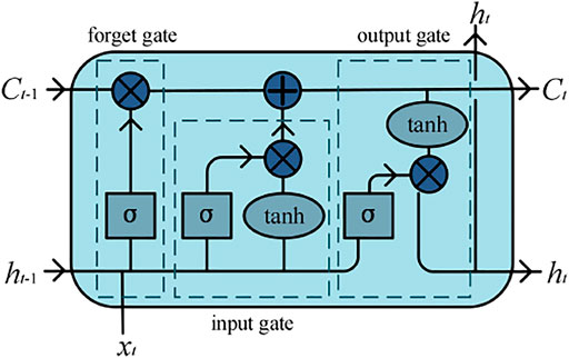
FIGURE 2. Basic unit model of LSTM.

The forget gate determines the degree of retention of historical state information. When the output value is closer to 0, it means more discarded; when the output value is closer to 1, it means more reserved as follows:

$f_t=\mathrm{sigmoid}({\mathit{w}}_{\mathrm{f}}\cdot [h_{t-1},x_t]+{\mathit{b}}_{\mathrm{f}})(10)$

where x_t denotes the input vector. h_t-1 denotes the output vector of the hidden layer at the previous moment. w_f and b_f denote the weight and bias of the forget gate, respectively.

The input gate determines the information stored in the unit as follows:

$i_t=\mathrm{sigmoid}({\mathit{w}}_{\mathrm{i}}\cdot [h_{t-1},x_t]+b_i)(11)$

Update the status information after getting the output value of the input gate. Then, the state and the new cell state calculate can be gained:

$C_t^{\prime }=\tanh ({\mathit{W}}_{\mathrm{c}}\cdot [h_{t-1},x_t]+b_c)(12)$

$C_t=f_t\ast C_{t-1}+i_t\ast C_t^{\prime }(13)$

where w_i and w_c denote the weights of the input gate and cell state, respectively. b_i and b_c denote the biases of the input gate and cell state, respectively.

The output gate determines the output of information:

$o_t=\mathrm{sigmoid}({\mathit{w}}_{\mathrm{o}}\cdot [h_{t-1},x_t]+b_o)(14)$

$h_t=o_t\ast \tanh \left(C_t\right),(15)$

where w_o denotes the weight of the output gate and b_o represents the bias of the output gate.

Prediction Method of Smooth Components

Compared with the fluctuant components, the data of each subsequence in the smooth components are extremely steady. ARIMA can be used to predict the smooth components, which can reduce time consumption while obtaining extremely high prediction accuracy. The ARIMA (p, d, q) model is shown as follows:

$\mathrm{\Delta }x=x_t-x_{t-1}=(1-D)x_t(16)$

${\mathrm{\Delta }}^{2}x=\Delta \mathrm{x}-\mathrm{\Delta }{x}_{t-1}={(1-D)}^2{x}_t(17)$

${\mathrm{\Delta }}^{d}x={(1-D)}^d{x}_t={\phi }_0+{\phi }_1{x}_{t-1}+{\phi }_2{x}_{t-2}\mathrm{...}+{\phi }_p{x}_{t-p}+{\epsilon }_t-{\theta }_1{\epsilon }_{t-1}\mathrm{...}-{\theta }_q{\epsilon }_{t-q}(18)$

where p denotes the autoregressive order; q denotes the average moving order; d denotes the difference order; φ₀, φ₁ … φ_p denote the autoregressive coefficients; and θ₁, θ₂ … θ_q denote the moving average coefficients.

Combined Prediction Method

In this section, the missing data in the historical data of regional wind power will be repaired and the data will be denoised to improve the signal-to-noise ratio. Then, the left and right end points of the data will be extended and decomposed by CEEMDAN. Additionally, we will delete the data of the extension part of each subsequence.

Forecasting Process

The CEEMDAN process will find the upper and lower envelopes, respectively, according to the maximum and minimum points of the repaired original sequence. When the training data are updated, they need to be re-decomposed, and subsequences will also change after each decomposition. Figure 3 shows that the decomposed IMFs₁ of the training data are separated by 96 data points. It can be seen that the changing trends of the overlapping part are almost the same, but a more obvious difference can be seen after partial magnification. Therefore, the trained model cannot be saved for continuous prediction. After each prediction is completed, the data need to be decomposed again by CEEMDAN, with the fluctuant/smooth components redivided and retrained. In addition, in order to directly obtain multiple power values, the LSTM model is trained in n:1 multi-input and multi-output modes. After the model training is completed, the last n data are input, and the future l data will be predicted.

FIGURE 3

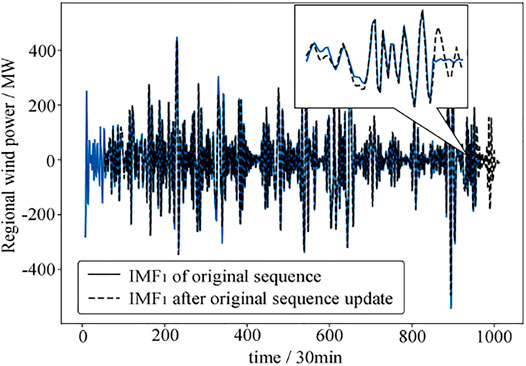
FIGURE 3. Difference of IMF1 before and after updating training data.

The construction process based on the fluctuant /smooth components partition model (combined prediction method) is shown in Figure 4. The specific steps are as follows:

1) Extract the repaired n days of historical data before the predictive time points as the training data, and complete the data extension.

2) Perform CEEMDAN on the data to obtain the subsequences composed of IMFs and Res. Calculate the proportion f of each subsequence, and divide IMFs and Res into fluctuant components and smooth components according to f.

3) Different methods are used to model the subsequences contained in the fluctuant components and the smooth components.

FIGURE 4

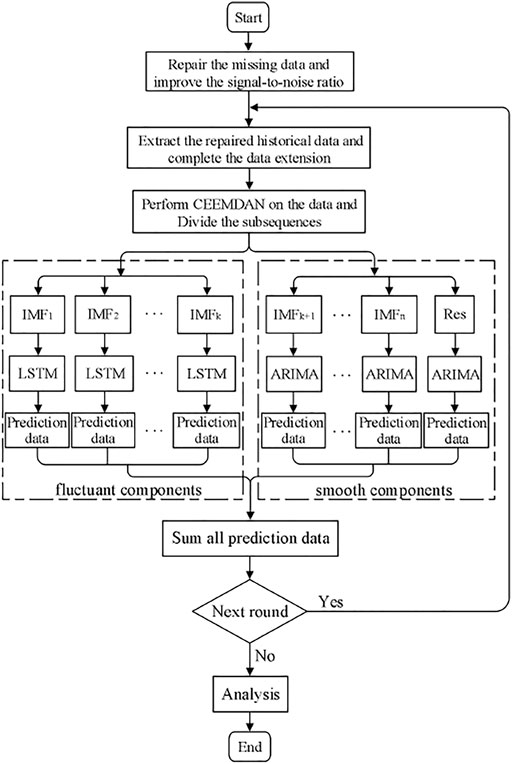
FIGURE 4. Prediction flow chart based on fluctuant/smooth components division.

For the fluctuant components, each subsequence is divided into training data and testing data. The tree-structured Parzen estimator (TPE) algorithm is used to optimize the hyperparameters of the LSTM model, including the number of LSTM layers of each model, the number of nodes in each layer, the activation function, batch_size, and optimizer.

For the smooth components, ARIMA (1, 2, 0) is used to fit the z data points before each subsequence predictive time point. After the fitting function is obtained, the z + 1 to z + l data can be calculated.

4) The final predictive result can be obtained by combining all the predictive data for each subsequence.

5) In the next round of prediction, update the regional wind power historical data first and repeat Steps 1–4 to start a new prediction round. The hyperparameter optimization process of the LSTM model is not re-optimized due to the time-consuming process, and the first hyperparameters combination is used again.

Evaluation Indexes

In order to measure the prediction accuracy, an evaluation system with mean absolute error (MAE), root mean squared error (RMSE), and qualified rate (Q) is established, which can effectively reflect the prediction accuracy. The calculations of MAE, RMSE, and Q are shown in Eqs 19, 20, 21, 22. RMSE and MAE reflect the absolute value of the error and are used to directly measure the prediction accuracy. Q reflects the acceptable degree of the prediction effect in practice.

$\mathrm{MAE}=\frac{1}{n}{\displaystyle \sum _{i=1}^n\left|P_{\mathrm{p}}-P_{\mathrm{r}}\right|}(19)$

$\mathrm{RMSE}=\sqrt{\frac{1}{n}{\displaystyle \sum _{i=1}^n{(P_{\mathrm{p}}-P_{\mathrm{r}})}^2}}(20)$

${\eta }_i=\{\begin{array}{l}1\left|\frac{P_{\mathrm{p}}-P_{\mathrm{r}}}{P_{\mathrm{r}}}\right|<10\%\\ 0\left|\frac{P_{\mathrm{p}}-P_{\mathrm{r}}}{P_{\mathrm{r}}}\right|\ge 10\%\end{array}(21)$

$\mathrm{Q}=\frac{1}{n}\left({\displaystyle \sum _{i=1}^n{\eta }_i}\right)\times 100\%(22)$

where P_p denotes the prediction value, P_r denotes the real value, and n denotes the length of the prediction value.

Experiment

The data from lots of wind power plants in a certain area of northern China are extracted from the November and December data of the current year. The unit is MW and the time resolution is 30 min. Therefore, there are 48 regional wind power values each day.

Historical Data Acquisition and Processing

Wind power data have strong intermittentness, randomness, and volatility, making it difficult to obtain high prediction accuracy for ultra-short-term wind power prediction. The curve in Figure 5 is the regional wind power data within 1 month. It can be seen that the data do not have obvious regularity but have a wide range of changes. The ultra-short-term sudden rise and sudden rise of nearly 4000 MW can be achieved within half a day. It also explains the low prediction accuracy of most algorithm models to a certain extent.

FIGURE 5

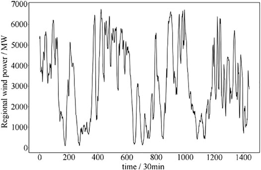
FIGURE 5. Variation of regional wind power data.

In each prediction, 960 wind power data points for 20 days are selected as the training data, and the prediction period is from 00:00 to 06:00 on the 21st day. Thirty-five comparative experiments have been conducted. The decomposition of the first CEEMDAN is made after removing the extension data, and six groups of IMFs and Res with frequency from high to low are obtained in Figure 6.

FIGURE 6

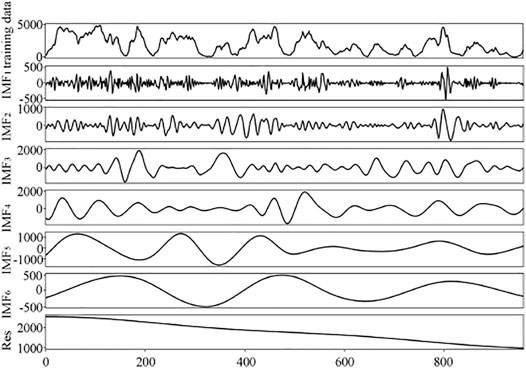
FIGURE 6. Decomposition effect of CEEMDAN.

Figure 6 shows that the change of each subsequence is relatively stable, and there is no obvious modal aliasing phenomenon, which is in line with the expected assumption. Based on many experiments, we decided to set 2% as the component division threshold f*. When the f of subsequence is greater than 2%, this subsequence is divided into fluctuant components. When the f of subsequence is less than 2%, this subsequence is divided into smooth components. With respect to the smooth components, using ARIMA instead of LSTM can not only eliminate the complex parameter tuning but also make the calculation faster. In Figure 6, from IMF₁ to IMF₄ belong to the fluctuant components, and the rest belong to the smooth components.

The total number of subsequences decomposed during 35 ultra-short-term predictions are shown in Figure 7. The numbers of subsequences are relatively stable, which are all between six and eight. Among them, seven groups had 25 times at most, accounting for 71.428%. Eight groups and six groups had six times and four times, respectively, accounting for 17.143% and 11.429% of the total. This also shows that after the training data are updated, the subsequence data decomposed by CEEMDAN are relatively stable, and there is no obvious difference in volatility. Therefore, it is reasonable for LSTM to train the subsequence following the first optimized hyperparameters.

FIGURE 7

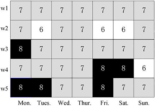
FIGURE 7. Number of decomposed subsequences of CEEMDAN.

Analysis of Prediction Results

In order to compare the performance of the combined prediction method in regional ultra-short-term wind power forecasting, ARIMA, SVR, BP, and LSTM are selected as comparative models, and actual project forecast data are added as a reference. The neural network model can obtain multiple outputs. BP and LSTM models all use 48 inputs and 12 outputs to train the models and use the TPE algorithm to determine the hyperparameters. Specifically, the hidden layer of BP is set as two layers with 36 neurons and 18 neurons, and the optimizer, activation function, and batch_size are Adam, tanh, and 64, respectively. For LSTM, the hidden layer is set as two layers with 48 neurons and 18 neurons. The optimizer, activation function, and batch_size are set to nadam, tanh, and 32. Moreover, the ARIMA and SVR models use rolling predictions to obtain 12 forecast data and use the grid search to achieve the best hyperparameters. The hyperparameters of the comparative model are optimized, and the results are as follows. p, d, and q of ARIMA are set as 4, 1, and 0, respectively. The kernel function, c, and epsilon of SVR are set as a linear kernel function, 1, and 0.05.

Table 1 shows the statistical results of the regional ultra-short-term wind power prediction within 1 month.

TABLE 1

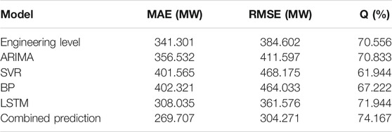
TABLE 1. | Model prediction accuracy comparison.

In Table 1, the combined prediction model has the best prediction effect when the hyperparameters of all the models are selected according to their respective optimization strategies. Compared with the engineering level, ARIMA, SVR, BP, and LSTM, the MAE of the combined prediction model is lower by 71.594, 86.825, 131.858, 132.614, and 38.328 MW, respectively. The RMSE is lower by 80.331, 107.326, 163.904, 159.762, and 57.305 MW, respectively. Q is higher by 3.611%, 3.334%, 12.223%, 6.945%, and 2.223% respectively. It indicates that CEEMDAN can effectively decompose the regional wind power historical data into several regular subsequences. At the same time, the fluctuant and smooth components are modeled by different methods, which can give full play to the predictive capabilities of LSTM and ARIMA. Figure 8 is a comparison of the prediction results for 1 day. The combined prediction results are the closest to the real value, which can effectively follow the 12 points of wind power in the next 6 h.

FIGURE 8

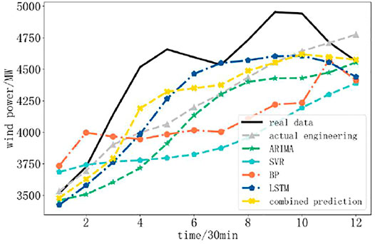
FIGURE 8. Comparison of prediction results.

Figures 9–11 give the box diagram of MAE, RMSE, and Q. It can be shown that the box height of the combined prediction model is the lowest among all the models, which demonstrates that the prediction error of the combined prediction model is more concentrated. In addition, in Figures 9, 10, the lower quartile line, the upper quartile line, and the upper edge of the combined prediction model are lower than those of other models except for LSTM, which indicates that the changes in the MAE and RMSE of the combined prediction model are concentrated, and the error is generally lower than other models. Figure 11 shows that the lower quartile of the combined prediction model is also the highest among all models, and the median line is also higher than most models, which indicates that the Q of the combined prediction model is generally higher than other models. To sum up, the box diagrams for MAE, RMSE, and Q show that the combined prediction model is not the best in all aspects but can achieve a high prediction concentration.

FIGURE 9

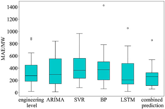
FIGURE 9. MAE box diagram of each model.

FIGURE 10

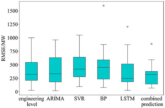
FIGURE 10. RMSE box diagram of each model.

FIGURE 11

FIGURE 11. Q box diagram of each model.

Conclusion

According to the variation characteristics of historical data of the regional wind power, this study proposes a combined prediction method based on CEEMDAN and the division of fluctuant/smooth components. The following studies have been completed.

1) In order to deeply explore the variation of historical data of the regional wind power, CEEMDAN is selected to decompose the data after extension processing, and the subsequences obtained are divided into the fluctuant and smooth components. LSTM is used to train the subsequences of the fluctuation components, while ARIMA is used to fit the subsequences of the smooth components directly. This method not only remedies the defect of the regularity of the regional wind power data but also gives full play to the advantages of LSTM and ARIMA.

2) The example shows that the combined prediction model can better follow the variation of the regional wind power data and can effectively improve the ultra-short-term prediction accuracy of regional wind power.

In this article, the prediction speed needs to be improved. It is proposed to further study the neural network with a simple structure to realize fast prediction, such as the improved method based on GRU.

Data Availability Statement

The original contributions presented in the study are included in the article/Supplementary Material, Further inquiries can be directed to the corresponding author.

Author Contributions

Conceptualization: YL and LY; methodology: YL and LY; software: YL and LY; validation: YL, WZ, and LY; formal analysis: YL; investigation: LY; resources: YL; data curation: HH; writing—original draft preparation: LY; writing—review and editing: YL, WZ, and LY; visualization: LY. All authors have read and agreed to the published version of the manuscript.

Funding

This research was funded by the National Natural Science Foundation of China (61703405).

Conflict of Interest

HH was employed by State Grid Jiangxi Electric Power Co., Ltd.

The remaining authors declare that the research was conducted in the absence of any commercial or financial relationships that could be construed as a potential conflict of interest.

Publisher’s Note

All claims expressed in this article are solely those of the authors and do not necessarily represent those of their affiliated organizations or those of the publisher, the editors, and the reviewers. Any product that may be evaluated in this article, or claim that may be made by its manufacturer, is not guaranteed or endorsed by the publisher.

References

Bedi, J., and Toshniwal, D. (2018). Empirical Mode Decomposition Based Deep Learning for Electricity Demand Forecasting. IEEE Access 6, 49144–49156. doi:10.1109/access.2018.2867681

CrossRef Full Text | Google Scholar

Chen, W., Qi, W., Li, Y., Zhang, J., Zhu, F., Xie, D., et al. (2021). Ultra-Short-Term Wind Power Prediction Based on Bidirectional Gated Recurrent Unit and Transfer Learning. Front. Energ. Res. 9, 808116. doi:10.3389/fenrg.2021.808116

CrossRef Full Text | Google Scholar

Elsaraiti, M., and Merabet, A. (2021). Application of Long-Short-Term-Memory Recurrent Neural Networks to Forecast Wind Speed. Appl. Sci. 11, 2387. doi:10.3390/app11052387

CrossRef Full Text | Google Scholar

Fu, Q., Jing, B., He, P., Si, S., and Wang, Y. (2018). Fault Feature Selection and Diagnosis of Rolling Bearings Based on EEMD and Optimized Elman_AdaBoost Algorithm. IEEE Sensors J. 18, 5024–5034. doi:10.1109/jsen.2018.2830109

CrossRef Full Text | Google Scholar

Gan, L., Li, G. Y., and Zhou, M. (2016). Coordinated Planning of Large-Scale Wind Farm Integration System and Transmission Network. CSEE J. Power Energ. Syst. 2, 2530–2539. doi:10.17775/cseejpes.2016.00005

CrossRef Full Text | Google Scholar

Hochreiter, S., and Schmidhuber, J. (1997). Long Short-Term Memory. Neural Comput. 9, 1735–1780. doi:10.1162/neco.1997.9.8.1735

PubMed Abstract | CrossRef Full Text | Google Scholar

Huang, N. E., Shen, Z., Long, S. R., Wu, M. C., Shih, H. H., Zheng, Q., et al. (1998). The Empirical Mode Decomposition and the hilbert Spectrum for Nonlinear and Non-stationary Time Series Analysis. Proc. R. Soc. Lond. A. 454, 903–995. doi:10.1098/rspa.1998.0193

CrossRef Full Text | Google Scholar

Huang, N. E., Wu, M.-L. C., Long, S. R., Shen, S. S. P., Qu, W., Gloersen, P., et al. (2003). A Confidence Limit for the Empirical Mode Decomposition and hilbert Spectral Analysis. Proc. R. Soc. Lond. A. 459, 2317–2345. doi:10.1098/rspa.2003.1123

CrossRef Full Text | Google Scholar

Liu, Y., Guan, L., Hou, C., and Han, H. (2019). Wind Power Short-Term Prediction Based on LSTM and Discrete Wavelet Transform. Appl. Sci. 9, 1108. doi:10.3390/app9061108

CrossRef Full Text | Google Scholar

Lobo, M. G., and Sanchez, I. (2012). Regional Wind Power Forecasting Based on Smoothing Techniques, with Application to the Spanish Peninsular System. IEEE Trans. Power Syst. 27, 1990–1997. doi:10.1109/tpwrs.2012.2189418

CrossRef Full Text | Google Scholar

Lu, P., Ye, L., Tang, Y., Zhao, Y., Zhong, W., Qu, Y., et al. (2021). Ultra-short-term Combined Prediction Approach Based on Kernel Function Switch Mechanism. Renew. Energ. 164, 842–866. doi:10.1016/j.renene.2020.09.110

CrossRef Full Text | Google Scholar

Mahmoud, T. K., Dong, Z. Y., and Ma, J. (2017). A Developed Integrated Scheme Based Approach for Wind Turbine Intelligent Control. IEEE Trans. Sustain. Energ. 8, 927–937. doi:10.1109/tste.2016.2632104

CrossRef Full Text | Google Scholar

Qu, Z. X., Mao, W. Q., Zhang, K. Q., Zhang, W. Y., and Li, Z. P. (2018). Multi-step Wind Speed Forecasting Based on a Hybrid Decomposition Technique and an Improved Back-Propagation Neural Network. Renew. Energ. 133, 919–929. doi:10.1016/j.renene.2018.10.043

CrossRef Full Text | Google Scholar

Safari, N., Chung, C. Y., and Price, G. C. D. (2017). Novel Multi-step Short-Term Wind Power Prediction Framework Based on Chaotic Time Series Analysis and Singular Spectrum Analysis. IEEE Trans. Power Syst. 33, 590–601. doi:10.1109/TPWRS.2017.2694705

CrossRef Full Text | Google Scholar

Torres, M. E., Colominas, M. A., Schlotthauer, G., and Flandrin, P. (2011). A Complete Ensemble Empirical Mode Decomposition with Adaptive Noise. Proceedings of the 2011 IEEE International Conference on Acoustics, Speech and Signal Processing. Prague: Czech Republic, 22–27. doi:10.1109/icassp.2011.5947265

CrossRef Full Text | Google Scholar

Wang, C., Zhang, H., Fan, W., and Ma, P. (2017). A New Chaotic Time Series Hybrid Prediction Method of Wind Power Based on EEMD-SE and Full-Parameters Continued Fraction. Energy 138, 977–990. doi:10.1016/j.energy.2017.07.112

CrossRef Full Text | Google Scholar

Wang, H.-z., Li, G.-q., Wang, G.-b., Peng, J.-c., Jiang, H., and Liu, Y.-t. (2017). Deep Learning Based Ensemble Approach for Probabilistic Wind Power Forecasting. Appl. Energ. 188, 56–70. doi:10.1016/j.apenergy.2016.11.111

CrossRef Full Text | Google Scholar

Wang, L., Tao, R., Hu, H., and Zeng, Y.-R. (2021). Effective Wind Power Prediction Using Novel Deep Learning Network: Stacked Independently Recurrent Autoencoder. Renew. Energ. 164, 642–655. doi:10.1016/j.renene.2020.09.108

CrossRef Full Text | Google Scholar

Wang, P., Sun, Y. H., Thai, S. W., and Wu, X. P. (2019). Ultra Short Term Probability Prediction of Wind Power Based on Wavelet Decomposition and Long Short-Term Memory Network. In Proceedings of the 2019 31st Chinese Control and Decision Conference (CCDC 2019), Nanchang, China, 3-5, 2061–2066.doi:10.1109/ccdc.2019.8832903

CrossRef Full Text | Google Scholar

Wu, Q., Guan, F., Lv, C., and Huang, Y. (2021). Ultra‐short‐term Multi‐step Wind Power Forecasting Based on CNN‐LSTM. IET Renew. Power Generation 15, 1019–1029. doi:10.1049/rpg2.12085

CrossRef Full Text | Google Scholar

Wu, Z., and Huang, N. E. (2011). Ensemble Empirical Mode Decomposition: a Noise-Assisted Data Analysis Method. Adv. Adapt. Data Anal. 01, 1–41. doi:10.1142/S1793536909000047

CrossRef Full Text | Google Scholar

Xu, H. Y., Chang, Y. Q., Wang, F. L., and Wang, S. (2021). Univariate and Multivariable Forecasting Models for Ultra-short-term Wind Power Prediction Based on the Similar Day and LSTM Network. J. Renew. Sust. Energ. 13, 063307. doi:10.1063/5.0027130

CrossRef Full Text | Google Scholar

Zalzar, S., Bompard, E., Purvins, A., and Masera, M. (2020). The Impacts of an Integrated European Adjustment Market for Electricity under High Share of Renewables. Energy Policy 136, 111055. doi:10.1016/j.enpol.2019.111055

CrossRef Full Text | Google Scholar

Zhang, P., Li, C., Peng, C., and Tian, J. (2020). Ultra-short-term Prediction of Wind Power Based on Error Following Forget Gate-Based Long Short-Term Memory. Energies 13, 5400. doi:10.3390/en13205400

CrossRef Full Text | Google Scholar