Study of Supercritical CO2 Physical Property Calculation Models

The supercritical CO₂ (SC-CO₂) thermodynamic cycle has been a promising and revolutionary technology. Related research has put higher demands on CO₂ physical property calculations in terms of computational accuracy and speed. In this study, the deviations between the experimental data and predicted data calculated by several models of CO₂ physical property calculation were obtained. According to the comparison results, the Span–Wagner equation of state, the Vesovic model, and the free-volume viscosity model are selected to construct a set of high-precision CO₂ property calculation models. For the time-consuming problem of commonly used models, new models were developed by using the polynomial fitting and interpolation method, which improved the speed of the physical property calculation by five orders of magnitude while ensuring high accuracy. On this basis, a physical property calculation program for the SC-CO₂ thermodynamic cycle could be developed, which can meet the demands of engineering applications in accuracy and calculation speed.

Introduction

In recent years, supercritical fluid (SCF) techniques have played a catalytic role in scientific research and engineering applications. In the food, pharmaceutical, and cosmetic industries, SCF extraction technology enables soluble components to be extracted from raw materials with high speed and efficiency, taking advantage of the unique properties above the critical point (Sodeifian et al., 2016a; Sodeifian et al., 2016b). SCFs have also been introduced into the biochemical and pharmaceutical industries to improve the bioavailability of drugs by producing nano- and micro-sized drug particles (Sodeifian et al., 2017; Sodeifian and Sajadian 2018; Sodeifian et al., 2018; Sodeifian et al., 2019) and to make it simpler to control the characteristics of the ultimate product by supercritical solvent impregnation (Ameri, Sodeifian, and Sajadian,2020). Meanwhile, supercritical dyeing technology has been used to prevent environmental pollution (water) and improve the performance of the pigments during the dyeing process (Ardestani et al., 2020).

In the field of energy and power, ultra-supercritical units have drawn much attention in recent years due to their energy-saving and emission reduction advantages (Wang 2015). In related studies, supercritical carbon dioxide (SC-CO₂) has been introduced into the new energy conversions as a low-pressure alternative to supercritical water. The critical pressure of carbon dioxide is moderate. In the pseudocritical region, CO₂ has the characteristics of large specific heat, low viscosity, and high compressibility, the utilization of which makes the SC-CO₂ thermodynamic cycle system compact and efficient, showing a promising future in the fields of advanced nuclear power (Huang and Wang 2012) and industrial waste heat recovery (Tao and Tao 2016).

In the SC-CO₂ thermodynamic cycle, the distortions of CO₂ properties in the pseudocritical region such as the isothermal compression coefficient are beneficial to reduce the power consumption of the compressor and improve the system efficiency but also pose a greater challenge for the calculation of the properties. Moreover, cycle analysis, the design of key thermodynamic processes, and components all place high demands on the physical properties of CO₂ (Yang et al., 2020). Therefore, how to calculate the thermodynamic and transport properties of CO₂ within the cycle conditions quickly and accurately has been a research focus.

However, the existing CO₂ property calculation models and CO₂ property calculation programs are no longer well suited to the needs of the rapid development of SC-CO₂ research. For example, the Span–Wagner equation of state (Span and Wagner 1996), recognized as the equation of state with the highest accuracy, is limited by its complex form, which means that it is time-consuming. The commonly used property database NIST REFPROP, which is based on the Span–Wagner equation, is hardly available to large-scale calculations owing to the low computational speed. In previous studies, some scholars have noticed such problems and have used polynomial fitting methods (Bahadori et al., 2009; Ouyang 2011) and neural network algorithms (Zhang et al., 2019) to obtain property prediction models with higher accuracy and calculation speed. Nevertheless, these available models do not correspond to the actual needs of the SC-CO₂ thermodynamic cycle in terms of applicable working conditions and solving methods, and little research work has concentrated on the efficiency evaluation of these models to prove their superiority of computational efficiency. Thus, it is necessary to develop new models differing from the existing ones and pay attention to computational speed comparison of the commonly used prediction models with that of the new models.

This study aims to meet the demands for accuracy and efficiency of CO₂ property calculation in the thermodynamic cycle. Meanwhile, a CO₂ physical property measurement experiment was conducted to obtain precise property data. On this basis, we compared the deviations between the experimental and predicted values of various CO₂ physical property calculation models and finally selected the Span–Wagner equation of state, the Vesovic model (Vesovic et al., 1990), and the free-volume viscosity model (Liu et al., 2013) to make up a set of high-precision CO₂ property calculation models. Also, to solve the time-consuming problem of traditional high-precision models, a high-speed calculation model of CO₂ physical properties was constructed by using the polynomial fitting and interpolation method, which also satisfies the requirement for accuracy.

Research on High-Precision CO₂ Property Models

Experiment in CO₂ Physical Property Measurement

Although much research has been done on CO₂ property data, few experimental studies have been conducted in the range of supercritical conditions. Thus, to obtain precise experimental data in the supercritical region, the experiment of CO₂ physical property measurement was carried out so that the accuracy of available models could be checked.

In this work, the density ($\rho$), isobaric specific heat ($c_p$), and viscosity ($\eta$) of CO₂ temperatures from 298.15 to 773.15 K and pressures from 7 to 14 MPa were measured through the U-tube vibration method (Jiang 2011), flow calorimeter (Liu et al., 2014; He et al., 2015), and capillary method (Liu et al., 2011), respectively. The physical property measurement experiment apparatus is shown in Figure 1.

FIGURE 1

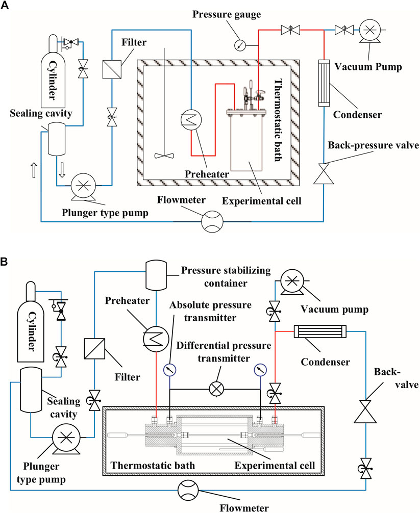
FIGURE 1. Schematic diagram of the experimental apparatus: (A) $c_p$ measurement (B) $\rho$ and $\eta$ measurement.

Several key technical problems have been solved in this experiment. First, a double-layer vacuum cylinder was used to ensure thermal insulation and prevent high temperature instability. Second, in order to minimize the heat loss, the fluid was heated by a microheater inside the tube assembly, and the heating tubes were fine. In addition, the horizontal placement of the experimental body proposed by Liu et al. (2014) was also used to avoid the vertical density stratification produced because of gravity.

Figure 2 presents the distribution of data points, where the horizontal and vertical coordinates indicate the temperature (in K) and pressure (in MPa), respectively. Table 1 summarizes the total measurement uncertainties of pressure and temperature, and the extended uncertainties at confidence factor k = 2 of $c_p$, $\rho$, and $\eta$. The uncertainty of $c_p$ comes from the measurement uncertainties of the differential temperature, the mass flow, the heating power, and the pressure. The uncertainty of $\rho$ is mainly from the uncertainty of the density measurement itself, and the uncertainty of $\eta$ is composed of the uncertainties of the inner diameter of the capillary tube, the mass flow, the differential pressure, the length of the capillary tube, the kinetic energy loss coefficient, the density, and the differential temperature. The equations for calculating synthetic uncertainty of $c_p$ and $\eta$ are as follows:

$u_c\left(c_p\right)=\sqrt{{\left(\frac{\partial c_p}{\partial \Delta T}\right)}^2{u}_{\Delta T}^2+{\left(\frac{\partial c_p}{\partial q_m}\right)}^2{u}_{q_m}^2+{\left(\frac{\partial c_p}{\partial Q}\right)}^2{u}_Q^2+{\left(\frac{\partial c_p}{\partial p}\right)}^2{u}_p^2},(1)$

$u_c \left(\eta \right)=\sqrt{{\left(\frac{\partial \eta }{\partial R}\right)}^2{u}_R^2+{\left(\frac{\partial \eta }{\partial q_m}\right)}^2{u}_{q_m}^2+{\left(\frac{\partial \eta }{\partial \Delta p}\right)}^2{u}_{\Delta p}^2+{\left(\frac{\partial \eta }{\partial L}\right)}^2{u}_L^2+{\left(\frac{\partial \eta }{\partial m}\right)}^2{u}_m^2+{\left(\frac{\partial \eta }{\partial \rho }\right)}^2{u}_{\rho }^2+{\left(\frac{\partial \eta }{\partial \Delta T}\right)}^2{u}_{\Delta T}^2,}(2)$

where $\Delta T$ is the differential temperature, $q_m$ is the mass flow, $Q$ is the heating power, $p$ is the pressure, $R$ is the inner diameter of the capillary tube, $\Delta p$ is the differential pressure, $L$ is the length of the capillary tube, $m$ is the kinetic energy loss coefficient, $\rho$ is the density, and $u_{factor}$ is the the uncertainty of some factors.

FIGURE 2

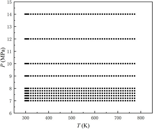
FIGURE 2. Distribution of experimental data points.

TABLE 1

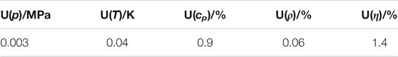
TABLE 1. Uncertainties of the experiment.

Selection and Evaluation Method

In this section, several commonly used models of CO₂ thermodynamic and transport properties were tested. $c_p$, $\rho$, and $\eta$ calculated by different models were compared with partial experimental data. According to the comparison results, the best performing models were selected. Furthermore, the selected models were evaluated with all the experimental data to reconfirm the accuracy.

Referring to Heidaryan and Jarrahian’s(2013) article, this article introduced four statistical parameters to present the comparison results, including the average relative error (ARE), average absolute relative error (AARE), absolute relative error (AE), and correlation coefficient (R²) (see Eq. 3–6):

$\text{ARE\%}=\frac{100}{{\text{N}}_{\text{d}}}\times {{\displaystyle \sum }}_{i=1}^{N_d}\left(\frac{{\rho }_{\text{i}}^{\text{exp}.}- {\rho }_{\text{i}}^{\text{calc}.}}{{\rho }_{\text{i}}^{\text{exp}.}}\right)(3)$

$\text{AARE\%}=\frac{100}{{\text{N}}_{\text{d}}}\times {{\displaystyle \sum }}_{i=1}^{N_d}\left|\frac{{\rho }_{\text{i}}^{\text{exp}.}- {\rho }_{\text{i}}^{\text{calc}.}}{{\rho }_{\text{i}}^{\text{exp}.}}\right|,(4)$

$\text{AE\%}=100\times \left|\frac{{\rho }_{\text{i}}^{\text{exp}.}- {\rho }_{\text{i}}^{\text{calc}.}}{{\rho }_{\text{i}}^{\text{exp}.}}\right|,\text{ and}(5)$

$R^2=1-\frac{{{\displaystyle \sum }}_{i=1}^{N_d}{\left({\rho }_{\text{i}}^{\text{exp}.}- {\rho }_{\text{i}}^{\text{calc}.}\right)}^2}{{{\displaystyle \sum }}_{i=1}^{N_d}{\left({\rho }^{\text{mean}}-{\rho }_{\text{i}}^{\text{calc}.}\right)}^2},(6)$

where ARE indicates the bias between the evaluated data and reference data. The smaller the ARE, the smaller the systematic bias of the data. When ARE is 0, it indicates that the values of evaluated data are randomly distributed around the reference data values. The AARE characterizes the accuracy of the evaluated data compared with the reference data. The maximum value of AE is the maximum deviation of the evaluated data from the reference data. The R² represents the precision of the evaluated data. The closer the R² is to 1, the stronger the correlation between the evaluated data and the reference data.

The specific selection criteria are as follows. Comparing data out of the pseudocritical region, a smaller AARE value and R² value closer to 1 indicate higher accuracy and precision of the model, respectively; if the values of these two statistical parameters are close between different models, then the AE (max) values in the pseudocritical region are compared, and the model with the smaller ones is counted as the better one.

Results and Discussion

Table 2 shows the comparisons between the predicted data obtained by different commonly used models and the experimental data out of the pseudocritical region. For $\rho$ and $c_p$ calculations, the AARE of the FEQ model (the Span–Wagner equation) is only 0.144 and 1.215%, respectively, and the R² are both close to 1. The values of these two parameters in contrast with those of other models indicate a high degree of accuracy and precision of the Span–Wagner equation in $\rho$ and $c_p$ calculations. For the calculation of $\eta$, the VS1 model and VS4 model have similar resultant values. The AAREs are 1.819 and 1.713%, and R² are both close to 1. Thus, to choose the better viscosity model, their predicted $\eta$ values are further compared with the experimental data in the pseudocritical region. The VS1 model (also the Vesovic model) is obtained to have a smaller AE value in the pseudocritical region overall (see Table 3).

TABLE 2

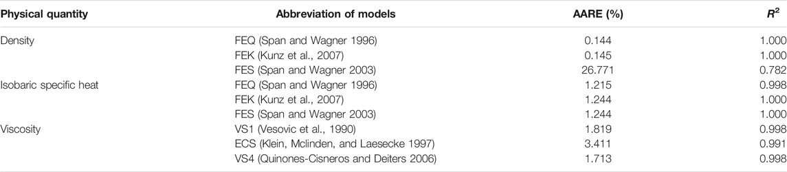
TABLE 2. Comparison between the predicted and experimental data out of pseudocritical region.

TABLE 3

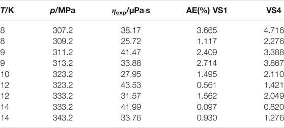
TABLE 3. Comparison between the predicted and experimental data in pseudocritical region.

In addition, for $\eta$ calculation, in order to make up for the shortcomings of the Vesovic model like complexity, the free-volume viscosity model with a simple form is introduced to this study. It is worth mentioning that several parameters of the model are obtained by fitting our experimental data, which means that it concentrates more on the supercritical region. Within that region (298.15 K≤ $T$ <773.15 K and seven MP a ≤ $p$ <14 MPa), its accuracy could be good. The equations are as follows (Liu et al., 2013):

$\eta ={\eta }_0+\Delta \eta ,(7)$

where

${\eta }_0=4.0785\times \frac{\sqrt{MT}}{V_c^{\frac{2}{3}}{\Omega }^{\ast }\left(T^{\ast }\right)}{F}_c\text{ and}(\mathrm{7a})$

$\Delta \eta =\frac{\rho l\left(\alpha \rho +\frac{pM}{\rho }\right)}{\sqrt{3RTM}}\exp \left[B{\left(\frac{\alpha \rho +\frac{pM}{\rho }}{RT}\right)}^{\frac{3}{2}}\right],(\mathrm{7b})$

where ${\eta }_0$ is the viscosity of dilute gas, $\Delta \eta$ is the correction term for the viscosity of dense fluid, ${\Omega }^{\ast }$ is the collision integral, $F_c$ is the parameter related to dipole moment and eccentricity factor, $B$ is the superimposed part of the free volume, $M$ is the molar mass, $\alpha \rho$ is the energy barrier, $l=L^2/b_f$ is the $L^2$ is the molecular mean characteristic square length and $b_f$ is the dissipation of potential energy.

In the aforementioned equations, $\alpha$, $B$, and $l$ are obtained by fitting the experimental data, and the values are as follows: $\alpha$ = 13.34816839, $B=$ 8.04589798 × 10⁻¹¹, and $l=$ 0.03939321.

Finally, the Span–Wagner equation of state, the Vesovic model, and the free-volume viscosity model are chosen to construct a set of high-precision CO₂ property calculation models. The three selected high-precision models are further evaluated to analyze their accuracy. The experimental data (298.15 K≤ $T$ <773.15 K and seven MP a ≤ $p$ <14 MPa) are divided into data in the general region and pseudocritical region, and the calculated data and experimental data are compared on this basis, as shown in Table 4.

TABLE 4

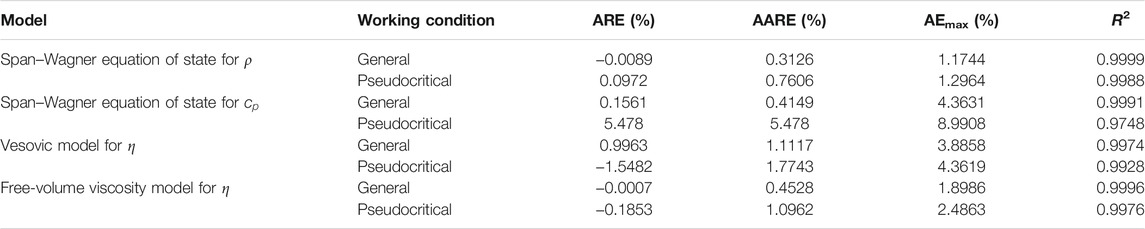
TABLE 4. Comparison of the calculated values of each model with the experimental data.

In the general region, the ARE between experimental data and the predicted $\rho$ calculated by the Span–Wagner equation is only -0.0089%, which is lower than the equation uncertainty ( $\pm$ 0.03%, $\pm$ 0.05%). In the pseudocritical region, although the average relative error is slightly larger than the equation uncertainty, it is still acceptable.

For $c_p$ calculation by the Span–Wagner equation, the ARE is only about 0.15% in the general region, while the maximum AE is 4.3631%, and this data point is near the pseudocritical region. The error around this region is generally large, possibly due to the rough partition of the pseudocritical region, which means that this part of general region is still influenced by property distortions. If data in the controversial region are ignored, the AARE then drops to about 1%. However, in the pseudocritical region, the ARE exceeds 5%, and the maximum AE is close to 9%. The absolute error between calculated and experimental values of $c_p$ in the pseudocritical region is presented in Table 5. The absolute error is large in the pseudocritical region from 7 to 8 MPa, up to 5.998 kJ/(kgK), indicating the poor accuracy of the Span–Wagner equation in the pseudocritical region.

TABLE 5

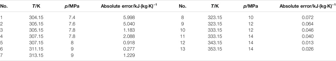
TABLE 5. Absolute error of isobaric specific heat calculation in the pseudocritical region.

For the comparison of $\eta$, the ARE between the Vesovic model and the experimental result is below the model’s minimum uncertainty of 1% in the general region. In the pseudocritical region, it is still lower than the uncertainty of 2% given by the model for this region. However, there are still several data points near the pseudocritical region with large AE up to 4%, suggesting that the $\eta$ calculation of the Vesovic model in the pseudocritical region is defective.

The free-volume viscosity model has very high accuracy in $\eta$ calculation throughout the region. The ARE is within 0.001% in the general region and only about 0.18% in the pseudocritical region.

These evaluation results offer some ideas for the improvement of the existing calculation programs. For example, in terms of CO₂ physical property calculation, the widely used program REFPROP is based partly on the Span–Wagner equation and the Vesovic model. The accuracy is relatively high as the evaluation results show. However, for the $\eta$ calculation in the supercritical region, it could be more accurate than the Vesovic model used by REFPROP when using the free-volume viscosity model.

Research on Fast Calculation CO₂ Property Models

In engineering applications of SC-CO₂, such as sub-channel studies and system analysis, their computational procedures require high precision and efficiency for physical property calculations. However, the aforementioned high-precision computational models are in a relatively complicated form and have low computation speed, which greatly limits their use in engineering. Therefore, models with faster computation speeds need to be studied. In this part, two fast calculation methods are introduced: polynomial fitting and interpolation method.

Polynomial Fitted Model

In previous studies, many researchers have obtained property calculation models with high prediction accuracy in a certain temperature and pressure range, using polynomial fitting methods (Ouyang 2011) and neural network algorithms (Zhang et al., 2019). However, these existing models do not correspond to our actual needs in terms of applicable working conditions and solving methods. Thus, a new model appropriate to related research needs to be fitted.

After trying various equation forms, we found that the fitted model obtained by the polynomial form of Eq. 8 is the best, and the prediction accuracy is extremely high in the required temperature and pressure range.

$z\left(x,y\right)={{\displaystyle \sum }}_{\text{i}=0}^{\text{n}}{C}_{\text{i}}\left(x\right)y^{\text{i}},(8)$

where

$C_{\text{i}}\left(x\right)={{\displaystyle \sum }}_{\text{j}=0}^{\text{n}}{D}_{\text{ij}}{x}^{\text{i}}.(\mathrm{8a})$

According to the actual demand of CO₂ physical properties for sub-channel studies and others, the model is designed to be applicable in the range 373.15 K≤ $T$ <773.15 K, 10 MPa≤ $p$ <20 MPa. Since the Span–Wagner equation and the Vesovic model are highly accurate in this range, the numerical fitting will be performed based on their calculation results.

Six fitted models are finally obtained in the form of Eq. 8, and the specific physical properties represented by $x$, $y$, $z$ and the value $n$ of each model are shown in Table 6. The table of the fitted coefficients $D_{\text{ij}}$ can be seen in Tables 7–12. According to the comparison results of relative errors between standard data and the fitted model with different maximum numbers of decimal digits (see Table 13), it was found that the relative errors generally decrease quickly when the number of decimal places is taken to four digits, and the reduction in relative errors is relatively small when going from 4 to 5 decimal places. Meanwhile, the accuracy of the result obtained by taking 5 decimal places is sufficient for our needs. Thus, the coefficients are retained to 5 decimal places in this article as shown in the tables.

TABLE 6

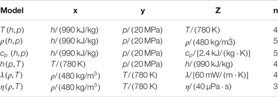
TABLE 6. Specific physical properties represented by x, y, z and the n value of each model.

TABLE 7

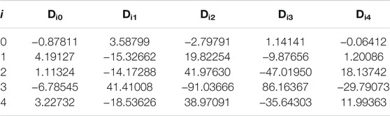
TABLE 7. Coefficients D_ij of $T\left(h,p\right)$.

TABLE 8

TABLE 8. Coefficients D_ij of $\rho \left(h,p\right)$.

TABLE 9

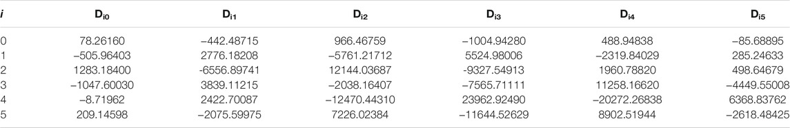
TABLE 9. Coefficients D_ij of $c_p \left(h,p\right)$.

TABLE 10

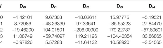
TABLE 10. Coefficients D_ij of $h\left(p,T\right)$.

TABLE 11

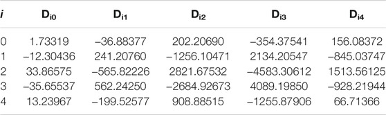
TABLE 11. Coefficients D_ij of $\lambda \left(\rho ,T\right)$.

TABLE 12

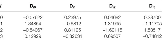
TABLE 12. Coefficients D_ij of $\eta \left(\rho ,T\right)$.

TABLE 13

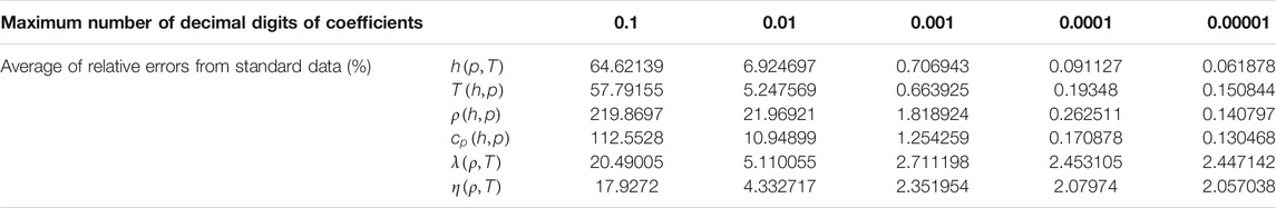
TABLE 13. Average of relative errors between standard data and the fitted models with different maximum number of decimal digits.

The deviation between the data by the fitted equations and the combination of the Span–Wagner equation and the Vesovic model outside the given applicable range (373.15 K≤ $T$ <773.15 K, 10 MPa ≤ $p$ <20 MPa) are calculated. Figure 3 shows that the distribution of the data points outside the given applicable range of the six equations, where the AE is less than 1 and 5%. The red and gray areas represent the range where the deviation is below 1 and 5%, respectively, and the surrounded blank area refers to the models’ applicable range. Under the accuracy requirement of 1%, the six equations are still acceptable in a wide range outside the applicable region, indicating that the calculation range of fitted models is expandable.

FIGURE 3

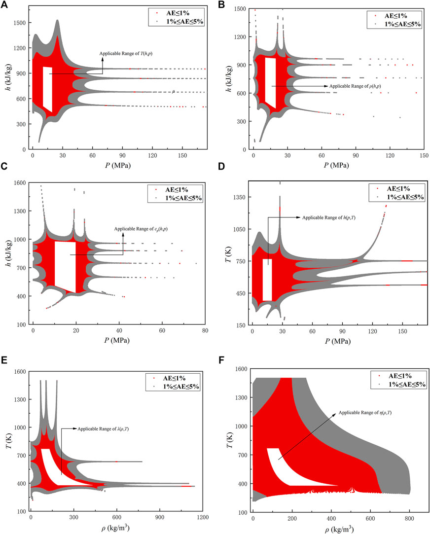
FIGURE 3. Distribution of working points with absolute error less than 1% for each formula: (A) $T\left(h,p\right)$ (B) $\rho \left(h,p\right)$ (C) $c_p\left(h,p\right)$ (D) $h\left(p,T\right)$ (E) $\lambda \left(\rho ,T\right)$ (F) $\mu \left(\rho ,T\right)$.

Fast Calculation Method: Interpolation

In addition to obtaining new models by polynomial fitting, interpolation is also a commonly used method with high computational speed. The basic idea is to estimate the physical properties through linear interpolation, referring to data tables of physical properties (interpolation nodes). It is fast but strictly limited to the range given by the data table, which means that it is non-expandable.

The applicable range, the physical properties to be calculated, and the corresponding independent variables are all consistent with those in the fitted models.

The values calculated by the fitted model and the interpolation method are compared with the predicted data calculated by the Span–Wagner equation and the Vesovic model. Table 14 presents the results: the maximum AE of them in the applicable range. The maximum AEs are all very small, within 2.02% (1% if disregarding $c_p$ calculation and the $\lambda$ interpolation calculation). The results indicate that both fitted models and the interpolation method have high accuracy. It can also be found that the fitted models generally have smaller maximum AE, which means that the accuracy of the fitted model is slightly higher than that of the interpolation method. However, considering the simplicity of the linear interpolation method compared to the fitted model calculation, the accuracy of the interpolation method is already satisfactory.

TABLE 14

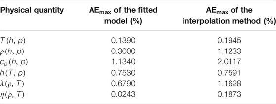
TABLE 14. Maximum absolute error between the two quick calculation methods and the standard data.

Computing Time Comparison With High-Precision Models

The fitted model, interpolation method, and the combination of the Span–Wagner equation and the Vesovic model are separately used to calculate the physical properties under 10⁵ working conditions in the applicable range, and the calculation time is compared as shown in Table 15, where CTR is the computing time ratio:

$CTR=\frac{\text{Calculation time of the Span}-\text{Wagner equation}}{\text{Calculation time of the fitted model }\left(\text{or the interpolation method}\right)}.(9)$

TABLE 15

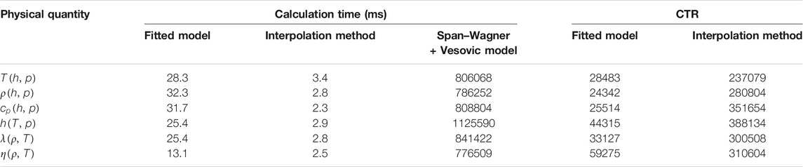
TABLE 15. Comparison of calculation time (for 10⁵ working conditions).

The computation time of the Span–Wagner equation + Vesovic model is four orders of magnitude more than that of the fitted models. and five orders of magnitude more than that of the interpolation method, showing the superiority of the two fast calculation models (methods) in terms of efficiency. In a cross-sectional comparison of the two fast calculation models (methods), it is found that the computation time of the interpolation method is only 1/10 of that of the fitted models. However, given that the overall accuracy of the interpolation method is slightly inferior to that of the fitted models, and the applicability is strictly limited to the given data tables, the choice of which calculation method to use should be combined with the reality in engineering applications.

Conclusion

Based on the experiment of CO₂ physical property measurement in the range of temperatures from 298.15 to 773.15 K and pressures from 7 to 14 MPa, some commonly used CO₂ property models are evaluated, and a set of relatively high-precision models is selected, including the Span–Wagner equation of state, the Vesovic model, and the free-volume viscosity model. Comparing $\rho$ (the Span–Wagner equation), $c_p$ (the Span–Wagner equation), and $\eta$ (the Vesovic model, the free-volume viscosity model) calculation results with experimental data, the AARE is 0.3126, 0.4149, 0.9963, and -0.0007, respectively, out of the pseudocritical region.

Meanwhile, to achieve the goal of fast calculation of CO₂ properties, polynomial fitting and interpolation methods are introduced in the present work. The results show that both methods have high accuracy with a relative error of less than 2.02% (1% if disregarding $c_p$ calculation and the $\lambda$ interpolation calculation) and can improve the calculation speed by 4-5 two magnitudes compared with the Span–Wagner equation + Vesovic model. Additionally, the fitted model has a large expandable region under the 1% accuracy requirement, and the computation time of the interpolation method is only 1/10 of that of the fitted models.

It can be concluded that the fitted models and interpolation method can successfully and quickly predict CO₂ properties within the range of temperatures from 373.15 to 773.15 K and pressures from 10 to 20 MPa. The results are significant for research of the SC-CO₂ Brayton cycle.

Data Availability Statement

The raw data supporting the conclusion of this article will be made available by the authors, without undue reservation.

Author Contributions

LM: Software, Formal Analysis, Writing - Original Draft; ML: Methodology, Writing - Review and Editing; DX: Software, Formal Analysis; MH and XL: Investigation, Validation; YH: Conceptualization, Funding Acquisition, Supervision.

Conflict of Interest

The authors declare that the research was conducted in the absence of any commercial or financial relationships that could be construed as a potential conflict of interest.

Publisher’s Note

All claims expressed in this article are solely those of the authors and do not necessarily represent those of their affiliated organizations, or those of the publisher, the editors, and the reviewers. Any product that may be evaluated in this article, or claim that may be made by its manufacturer, is not guaranteed or endorsed by the publisher.

References

Ameri, A., Sodeifian, G., and Sajadian, S. A. (2020). Lansoprazole Loading of Polymers by Supercritical Carbon Dioxide Impregnation: Impacts of Process Parameters. J. Supercrit. Fluids 164, 104892. doi:10.1016/j.supflu.2020.104892

CrossRef Full Text | Google Scholar

Bahadori, A., Vuthaluru, H. B., and Mokhatab, S. (2009). New Correlations Predict Aqueous Solubility and Density of Carbon Dioxide. Int. J. Greenhouse Gas Control. 3 (4), 474–480. doi:10.1016/j.ijggc.2009.01.003

CrossRef Full Text | Google Scholar

He, M., Su, C., Liu, X., Qi, X., and Lv, N. (2015). Measurement of Isobaric Heat Capacity of Pure Water up to Supercritical Conditions. J. Supercrit. Fluids 100, 1–6. doi:10.1016/j.supflu.2015.02.007

CrossRef Full Text | Google Scholar

Heidaryan, E., and Jarrahian, A. (2013). Modified Redlich⿿Kwong Equation of State for Supercritical Carbon Dioxide. J. Supercrit. Fluids 81, 92–98. doi:10.1016/j.supflu.2013.05.009

CrossRef Full Text | Google Scholar

Huang, Y., and Wang, J. (2012). Application of Supercritical Carbon Dioxide in Nuclear Reactor System. Nucl. Power Eng. 33 (3), 21–27. doi:10.1007/s11783-011-0280-z

CrossRef Full Text | Google Scholar

Jiang, Wei. (2011). Density Measurement by U-Tube Vibration Method. Sci. Tech. Inf. 000 (004), 1–2. doi:10.3969/j.issn.1672-3791.2011.04.001

CrossRef Full Text | Google Scholar

Klein, S. A., Mclinden, M. O., and Laesecke, A. (1997). An Improved Extended Corresponding States Method for Estimation of Viscosity of Pure Refrigerants and Mixtures. Int. J. Refrigeration 20 (3), 208–217. doi:10.1016/S0140-7007(96)00073-4

CrossRef Full Text | Google Scholar

Kunz, O., Klimeck, R., Wagner, W., and Jaeschke, M. (2007). The GERG-2004 Wide-Range Reference Equation of State for Natural Gases and Other Mixtures GERG TM15 2007. Germany: Düsseldorf VDI-Verl.

Google Scholar

Liu, X., He, M., and Zhang, Y. (2011). A Online Capillary Method for Viscosity Measurement under High Temperature and Pressure. J. Eng. Thermophys. 32 (8), 1283–1285.

Google Scholar

Liu, X., He, M. G., and Zhang, Y. (2013). Viscosity Model Based on the Free Volume Theory and the Crossover Function. J. Eng. Thermophys. V34 (001), 22–25.

Google Scholar

Liu, X., Su, C., He, K., and He, M. (2014). Measurement of Isobaric Heat Capacity of Pure Water at High Temperature and High Pressure. J. Eng. Thermophys. 35 (5), 844–847.

Google Scholar

Ouyang, L. B. (2011). New Correlations for Predicting the Density and Viscosity of Supercritical Carbon Dioxide under Conditions Expected in Carbon Capture and Sequestration Operations. Open Pet. Eng. J. 5 (1), 13–21. doi:10.2174/1874834101104010013

CrossRef Full Text | Google Scholar

Quiñones-Cisneros, S. E., and Deiters, U. K. (2006). Generalization of the Friction Theory for Viscosity Modeling. J. Phys. Chem. B 110 (25), 12820–12834. doi:10.1021/jp0618577

CrossRef Full Text | Google Scholar

Saadati Ardestani, N., Sodeifian, G., and Sajadian, S. A. (2020). Preparation of Phthalocyanine green Nano Pigment Using Supercritical CO2 Gas Antisolvent (GAS): Experimental and Modeling. Heliyon 6 (9), e04947. doi:10.1016/j.heliyon.2020.e04947

PubMed Abstract | CrossRef Full Text | Google Scholar

Sodeifian, G., Razmimanesh, F., and Sajadian, S. A.. 2019. Solubility Measurement of a Chemotherapeutic Agent (Imatinib Mesylate) in Supercritical Carbon Dioxide: Assessment of New Empirical Model. J. Supercrit. Fluids 146 89–99. doi:10.1016/j.supflu.2019.01.006

CrossRef Full Text | Google Scholar

Sodeifian, G., Saadati Ardestani, N., Sajadian, S. A., and Ghorbandoost, S. (2016a). Application of Supercritical Carbon Dioxide to Extract Essential Oil from Cleome Coluteoides Boiss: Experimental, Response Surface and Grey Wolf Optimization Methodology. J. Supercrit. Fluids 114, 55–63. doi:10.1016/j.supflu.2016.04.006

CrossRef Full Text | Google Scholar

Sodeifian, G., Sajadian, S. A., and Saadati Ardestani, N. (2017). Determination of Solubility of Aprepitant (An Antiemetic Drug for Chemotherapy) in Supercritical Carbon Dioxide: Empirical and Thermodynamic Models. J. Supercrit. Fluids 128, 102–111. doi:10.1016/j.supflu.2017.05.019

CrossRef Full Text | Google Scholar

Sodeifian, G., Sajadian, S. A., and Saadati Ardestani, N. (2016b). Optimization of Essential Oil Extraction from Launaea Acanthodes Boiss: Utilization of Supercritical Carbon Dioxide and Cosolvent. J. Supercrit. Fluids 116, 46–56. doi:10.1016/j.supflu.2016.05.015

CrossRef Full Text | Google Scholar

Sodeifian, G., and Sajadian, S. A. (2019). Utilization of Ultrasonic-Assisted RESOLV (US-RESOLV) with Polymeric Stabilizers for Production of Amiodarone Hydrochloride Nanoparticles: Optimization of the Process Parameters. Chem. Eng. Res. Des. 142, 268–284. doi:10.1016/j.cherd.2018.12.020

CrossRef Full Text | Google Scholar

Sodeifian, G., Sajadian, S. A., and Daneshyan, S.. 2018. Preparation of Aprepitant Nanoparticles (Efficient Drug for Coping with the Effects of Cancer Treatment) by Rapid Expansion of Supercritical Solution with Solid Cosolvent (RESS-SC). J. Supercrit. Fluids 140: 72–84. doi:10.1016/j.supflu.2018.06.009

CrossRef Full Text | Google Scholar

Span, R., and Wagner, W. (1996). A New Equation of State for Carbon Dioxide Covering the Fluid Region from the Triple‐Point Temperature to 1100 K at Pressures up to 800 MPa. J. Phys. Chem. Reference Data 25 (6), 1509–1596. doi:10.1063/1.555991

CrossRef Full Text | Google Scholar

Span, R., and Wagner, W. (2003). Equations of State for Technical Applications. III. Results for Polar Fluids. Int. J. Thermophys. 24 (1), 111–162. doi:10.1023/A:1022362231796

CrossRef Full Text | Google Scholar

Tao, X., and Tao, W. (2016). S-CO2 Waste Heat Recovery System. Construction Mater. Decoration, 226–227. doi:10.3969/j.issn.1673-0038.2016.51.149

CrossRef Full Text | Google Scholar

Vesovic, V., Wakeham, W. A., Olchowy, G. A., Sengers, J. V., Watson, J. T. R., and Millat, J. (1990). The Transport Properties of Carbon Dioxide. J. Phys. Chem. Reference Data 19 (3), 763–808. doi:10.1063/1.555875

CrossRef Full Text | Google Scholar

Wang, C. (2015). The Design of Brayton Circle for S-CO2 PBR and Reactor Core Thermodynamic Analysis. Harbin, China: Harbin Engineering University.

Google Scholar

Yang, F., Liu, H., Yang, Z., and Duan, Y. (2020). Working Fluid Thermophysical Properties of the Supercritical Carbon Dioxide Cycle. Therm. Power Generation 49 (No.40710), 27–35. doi:10.19666/j.rlfd.202006163

CrossRef Full Text | Google Scholar

Zhang, C., Jiang, J. B., and Peng, X. D. (2019). Comparison and Correction of CO2 Properties Model in Critical Region. CIESC J. 70 (8), 3058–3070. doi:10.11949/0438-1157.20190184

CrossRef Full Text | Google Scholar