Research on Energy Management of a Virtual Power Plant Based on the Improved Cooperative Particle Swarm Optimization Algorithm

Energy management of virtual power plants (VPPs) directly affects operators’ operating profits and is also related to users’ comfort and economy. In order to provide a reasonable scheme for scheduling each unit of the VPP and to improve the operating profits of the VPP, this study focuses on the optimization of VPP energy management under the premise of ensuring the comfort of flexible load users. First, flexible loads are divided into time-shiftable load (TL), power-variable load (PL), and interruptible load (IL), and their accurate power consumption models are established, respectively. Then, aiming at maximizing the operation profits of a VPP operator, an optimization model of VPP energy management considering user comfort is proposed. Finally, the improved cooperative particle swarm optimization (ICPSO) algorithm is applied to solve the proposed VPP energy management optimization model, and the optimal scheduling scheme of VPP energy management is obtained. Taking a VPP in the coastal area of China as an example, results show that the optimization model proposed in this article has the advantages of good economy and higher user comfort. Meanwhile, the ICPSO algorithm has the characteristics of faster optimization speed and higher accuracy when solving the problem with multiple variables.

Introduction

The problems of global energy crisis, climate warming, and environmental degradation have become increasingly prominent, which seriously threatens the survival and sustainable development of mankind (Yu et al., 2019; Elmorshedy et al., 2021). Developing renewable energy represented by wind energy and solar energy has gradually become an important way to protect the environment and lead the energy transformation (Hannan et al., 2021; Vohra and Sano, 2021). Wind power and photovoltaic power generation are widely used and popularized because of their advantages of low cost, no pollution, high flexibility, and high reliability (Mohammad et al., 2017). In 2019, the cumulative installed capacity of wind power and photovoltaic power generation in China will exceed 200 GW (Yang et al., 2020). However, due to uncertainties in natural factors such as wind speed and light intensity, wind turbines and photovoltaic power generation fluctuate greatly in time scale (Naughton et al., 2021). When large-scale new energy cannot be consumed locally, its grid connection will bring great challenges to the safe and stable operation of the power grid (Shabani and Kalantar, 2021). A VPP is a complex of renewable energy, energy storage system (ESS), conventional generator set, and adjustable load, and it is an effective way to realize local consumption of renewable energy (Luo et al., 2020; Dilantha et al., 2021). Through sensors, controllers, and communication networks, the VPP realizes the cooperative operation of its internal units and participates in electricity market transactions (Baringo et al., 2019). The operation mode of the VPP can optimize the overall energy efficiency and, at the same time, improve the economic benefits for various subjects (Zhang et al., 2021).

There are two modeling methods of VPP energy management: “top-down” and “bottom-up.” “top-down” is a modeling method based on existing operation data, which regards each unit in the VPP as an energy node and does not involve the mechanism model of a single unit (Zhao et al., 2018). Qu et al. put forward a comprehensive demand response model based on the price elasticity matrix, which explained the degree of influence of electricity consumption by electricity price, weather, day type, and other related factors (Qu et al., 2018). Li et al. compared and analyzed the VPP participation in the construction of the peak shaving and frequency modulation service market mechanism in different cities from four angles of market composition, market access, quotation clearing, and settlement and provided suggestions for the improvement of the VPP market mechanism (Li et al., 2021). “bottom-up” is a modeling method for constructing an equipment mechanism model based on factors such as equipment thermodynamic parameters and user behavior. Yoon et al. first established the mathematical model of residential air conditioning load and analyzed the response characteristics of monomer and polymerization load. On this basis, a linearized interactive demand response control strategy based on real-time electricity price was introduced to realize the control of a single air conditioning (Yoon et al., 2014). Zhu et al. first modeled the load of household appliances in detail and then developed a bottom-up residential electricity demand engineering model considering energy consumption and user comfort (Zhu et al., 2019). The “bottom-up” modeling method can more effectively reflect the effect of the control strategy. Combining the “top-down” and “bottom-up” modeling methods, this article establishes a VPP energy management model based on time of use tariff, which considers the subsidy cost of user comfort brought by applying flexible load adjustment and incorporates this cost into the objective function.

A VPP can carry out flexible load adjustment according to the hourly matching relationship between supply and demand of the system, so as to cope with the imbalance between supply and demand in some periods. Accurate description of flexible load can achieve the goals of less energy consumption, better economy, and higher user satisfaction (Yu et al., 2018). Mears and Martin considered the flexible load in the energy management of VPPs. By controlling the flexible load, the VPP can run more economically and stably. However, Mears and Martin did not analyze the accurate modeling of flexible load in detail (Mears and Martin, 2020). On the basis of considering IL and conventional load, Tan et al. established the VPP optimal scheduling model of carbon capture and waste incineration, which can effectively reduce the net cost and carbon emission of VPPs, realize the effective utilization of internal resources, and optimize the energy structure (Tan et al., 2021). Wang et al. considered TL and IL optimization in the VPP energy management system, but did not consider PL (Wang et al., 2020). In this article, PL is added to the existing research, and TL, PL, and IL are modeled more accurately.

The VPP energy management optimization problem is a nonlinear complex combinatorial optimization problem. For this kind of problem, the mixed integer quadratic programming method is often used to solve the model. However, because the VPP energy management model has many dimensions of variables, applying this method to solve the problem will bring about a double increase in computation and a “dimension disaster.” However, when solving nonlinear problems, the meta-heuristic algorithm does not need to transform nonlinear problems into linear problems, and its dimensions will not be multiplied. It can effectively deal with the solution of multidimensional models and can approach the optimal solution more quickly than the mixed integer quadratic programming method. Yang et al. used the multi-objective particle swarm optimization algorithm to solve the optimal real-time power allocation in the hybrid energy storage system (Yang et al., 2019). In the study by Mellouk et al. (2019), a parallel hybrid genetic algorithm was proposed to solve the energy management problem of the microgrid. In addition to the above two algorithms, other heuristic methods can be used to solve such problems, such as ant colony optimization (ACO) (Liang et al., 2020), artificial fish swarm algorithm (Zhang et al., 2019; Tirkolaee et al., 2020), and grey wolf optimization algorithm (Azizivahed et al., 2017). Among these heuristic methods, the particle swarm optimization (PSO) has become the preferred algorithm for solving complex nonlinear and nonconvex problems (Lin et al., 2009) because of its simple structure and few adjustment parameters (Charalampakis and Tsiatas, 2019). When using the standard PSO algorithm to solve the energy management problem of VPPs, each particle must include the adjustment schedule of all power generation and consumption equipment in VPPs. The PSO algorithm will encounter the problem of “two steps forward and one step backward” (Bergh and Engelbrecht, 2004), that is, when the optimization is carried out to a certain extent, due to the huge dimensions of particles, some dimensions of particles are close to the optimal solution, while the remaining dimensions are far from the optimal solution. In order to optimize the dimensions that deviate from the optimal solution, there is a certain chance that the dimensions that are close to the optimal solution will deviate from the optimal solution, resulting in difficulties in convergence. In order to overcome this difficulty, the cooperative particle swarm optimization (CPSO) algorithm was proposed in the study by Bergh and Engelbrecht (2004), which was implemented using the method of “divide and conquer.” The CPSO algorithm divides a day’s unit adjustment schedule into several continuous parts, each part is optimized by a particle swarm, and each subgroup iterates in sequence, which can speed up convergence. However, when particle precocity occurs, the slight deficiency of the first population will cause the fitness function of the last population to change seriously, and then all subgroups will fall into the local optimal state. In order to solve the problems in the CPSO algorithm, many methods to improve the CPSO algorithm have been proposed. Zhu et al. proposed the CPSO algorithm with particle reinitialization, but reinitialization will reduce the performance of the algorithm (Zhu et al., 2015). Riget and Vesterstrøm put forward a particle attraction and repulsion method to improve the CPSO algorithm, but the probability function of this method was fixed on the number of iterations, so this algorithm could not adapt well to the change of particle diversity (Riget and Vesterstrøm, 2002). In this study, a simulated annealing formula is introduced into the CPSO, and annealing is selected based on the probability function of particle diversity. Starting from a higher initial temperature and with the decrease in temperature parameters, the global optimal solution of the objective function is randomly selected in the feasible region with a certain probability, thus increasing the diversity of particles and avoiding premature particles.

Therefore, based on the ICPSO algorithm, a VPP energy management model considering user comfort is established in this article. The main contributions can be summarized as follows: 1) TL, PL, and IL are accurate, the adjustable potential of multiple types of loads is fully exploited, the influence mechanism of power market transaction on flexible load adjustment is revealed, and the cooperative and complementary relationship of different types of flexible loads in the adjustment process is obtained. 2) Considering the cost of flexible load adjustment, a complex nonlinear VPP energy management model is established with the goal of maximizing the overall operating income of the VPP, which achieves the goal of improving the operating income of the VPP without significantly affecting the comfort of users. 3) Based on the diversity of particles, a simulated annealing formula is introduced into the CPSO algorithm, and the ICPSO is proposed, which improves the global search ability of the algorithm.

The following main contents of this article can be summarized as follows: Section 2: Basic principles and flexible load modeling of the virtual power plant; Section 3: Energy management model of the virtual power plant; Section 4: Improved cooperative particle swarm algorithm; Section 5: Case introduction; Section 6: Analysis of optimization results; Section 7: Conclusion.

Basic Principle of Virtual Power Plant and Flexible Load Modeling

Basic Principles of Virtual Power Plant

A VPP is a cooperative polymer including power generation equipment, power consumption equipment, and energy storage equipment. The generator sets in the VPP include fossil energy generator sets and distributed new energy generator sets such as wind power and photovoltaic power generation. The electrical equipment is flexible load with adjustable characteristics and also includes energy storage equipment. The VPP operation mode is to realize interactive transactions between generator sets, flexible loads, and the electricity market by controlling the output of power generation equipment and adjusting flexible loads and to participate in the power grid demand response while consuming new energy generation. Its operation structure is shown in Figure 1.

FIGURE 1

FIGURE 1. Structure of a typical VPP.

Flexible Load Modeling

According to the load scheduling mode, this article divides the flexible load into TL (such as washing machine, dishwasher, etc.), PL (such as air conditioning, water heater, etc.), and IL (such as lighting, production load, etc.).

TL refers to the load that can change the energy consumption time within a scheduling period, where the load power shifted from t period to t' period can be expressed as follows:

$P_{TL}\left(t,t\prime \right)=N_{TL}\left(t,t\prime \right)\cdot \Delta P_{TL}(1)$

where P_TL (t, t′) is the load shift power from t period to t' period; N_TL (t, t′) is the shift load number from t period to t' period; ΔP_TL is the TL unit shift power.

When P_TL (t, t′) shifts to t' period, the load power of TL in t' period will increase correspondingly, which can be expressed as follows:

$P_{TL}\left(t\prime \right)=P_{TL}^0\left(t\prime \right)+P_{TL}\left(t,t\prime \right)(2)$

where P_TL (t′) is the TL load power in t' period after considering TL shift from t period to t' period; P0 TL (t') is TL load power in t' period before load adjustment.

PL refers to the load that changes its working power within the acceptable range of users, such as air conditioning, water heater, and other temperature control equipment. This study takes air conditioning as an example to establish a dynamic model of indoor temperature and PL load power.

$T_{in,i}(t+1)=T_{in,i}\left(t\right)e^{-1/(R\cdot C)}-\left(R\cdot P_{PL}^i\left(t\right)-T_{out}\left(t\right)\right)\cdot (1-e^{-1/(R\cdot C)})(3)$

where R is the thermal resistance of the building shell; C is the heat capacity of indoor air; Pi PL (t) is the working power of air conditioning equipment i in t period; T_in,i (t) is the indoor temperature of the building where air conditioning i is located in t period; T_out (t) is the outdoor temperature in t period.

After PL load adjustment, PL load power in t period can be expressed as follows:

$P_{PL}\left(t\right)={\displaystyle \sum }_{i=1}^{N_{PL}}{P}_{PL}^i\left(t\right)(4)$

where N_PL is the number of PL.

IL is a load that can directly interrupt its operation, and its adjustment model can be expressed as follows:

$P_{IL}\left(t\right)=P_{IL}^0\left(t\right)-N_{IL}\left(t\right)\cdot \Delta P_{IL}(5)$

where P_IL(t) is the IL load power after adjustment in t period; P0 IL (t) is the IL load power before adjustment in t period; N_IL (t) is the number of interrupted loads in t period; ΔP_IL is IL unit interrupt power.

Energy Management Model of Virtual Power Plant

Objective Function

On the premise of not significantly affecting user comfort, this study aims to maximize the profits of VPP operators, establishes a VPP energy management model, and optimizes the operation strategy of each unit in the VPP. After the power grid delivers the demand response task, the VPP responds to the power grid through load adjustment. During the power grid demand response period, the VPP will sell as much electricity as possible to the electricity market to complete the power grid demand response task.

In the non-demand response period of the power grid, VPP will absorb as much new energy as possible. The profit of VPP operators can be divided into sales revenue [I_SE (t)], income from participating in demand response [I_DR (t)], electricity purchase cost [C_BUY (t)], operation and maintenance cost [C_O&M (t)], flexible load adjustment cost [C_D (t)], and wind power and photovoltaic power generation cost [C_W&P (t)].

$\mathit{max}{\displaystyle \sum }_{t=1}^T\left(I_{SE}\left(t\right)+I_{DR}\left(t\right)-C_{BUY}\left(t\right)-C_{O\&M}\left(t\right)-C_D\left(t\right)-C_{W\&P}\left(t\right)\right)(6)$

1) Sales revenue, which includes the revenue from the VPP selling electricity to the electricity market and to load.

$I_{SE}\left(t\right)={\lambda }_{em}\left(t\right)G_{em}^{sell}\left(t\right)\Delta t+{\lambda }_{load}\left(t\right)P_{load}^{sell}\left(t\right)\Delta t(7)$

where λ_em (t) is the electricity price of the VPP selling to the electricity market in t period; Psell em (t) refers to the power that the VPP sells to the electricity market in t period; Δt is the time interval; λ_load (t) is the electricity price of the VPP for flexible load users in t period. Psell load (t) refers to the power that the VPP sells to flexible load users in t period.

2) Revenue obtained by participating in demand response. The VPP signs a demand response contract with the electricity market in advance to define the transaction power standard in each period. When the transaction standard is reached, the electricity market issues rewards to the VPP; otherwise, the electricity market imposes penalties on the VPP. Revenue obtained by VPP participation in demand response can be expressed as follows.

$I_{DR}\left(t\right)=\{\begin{array}{c}{c}_{up}\left(P_{em}^{sell}\left(t\right)-P_{em}^{std}\left(t\right)\right)+c_{std} P_{em}^{sell}\left(t\right)\ge P_{em}^{std}\left(t\right)\\ c_{dowm}\left(P_{em}^{sell}\left(t\right)-P_{em}^{std}\left(t\right)\right) P_{em}^{sell}\left(t\right)<P_{em}^{std}\left(t\right)\end{array}(8)$

where c_up is the reward for unit over-selling electricity when the transaction standard is reached; Pstd em (t) is the transaction power standard in t period; c_std is the basic reward for meeting the transaction standard; c_dowm is the penalty imposed when the transaction standard is not met.

3) Cost of electricity purchase. It is the cost of electricity purchase from the electricity market to the VPP.

$C_{BUY}\left(t\right)={\lambda }_{em}\left(t\right)P_{em}^{buy}\left(t\right)\Delta t(9)$

where Pbuy em (t) refers to the power purchased from the electricity market in t period.

4) System operation and maintenance cost, which consists of the operation and maintenance cost of ESS and conventional units.

$C_{O\&M}\left(t\right)=C_{ESS}\left(t\right)+C_G\left(t\right)(10)$

where C_ESS (t) and C_G (t) are, respectively, the operation and maintenance costs of ESS and conventional units in t period, which are calculated using the following formula.

ESS charging and discharging will cause loss to ESS, and its operation and maintenance cost can be expressed as follows.

$C_{ESS}\left(t\right)=a_{ESS}{P}_{ESS}^2\left(t\right)+b_{ESS}\left|P_{ESS}\left(t\right)\right|+c_{ESS}(11)$

where a_ESS, b_ESS, and c_ESS are, respectively, the quadratic, linear, and constant consumption characteristic parameters of ESS. P_ESS(t) is the charging and discharging power of ESS in t period. When it is positive, ESS is discharged and when it is negative, ESS is charged.

Operation and maintenance costs of conventional units can be expressed as follows.

$C_G\left(t\right)=c_G{P}_G\left(t\right)\Delta t+k_{oc}{P}_G\left(t\right)\Delta t+u_G\left(t\right)S_G(12)$

where c_G is the unit power generation cost of conventional units; P_G (t) is the output power of the conventional unit in t period; k_oc is the unit operation and maintenance cost of conventional units; u_G (t) is a Boolean variable, indicating whether the conventional unit is started in t period. When the unit changes from shutdown to running state in t period, u_G (t) is 1; otherwise, u_G (t) is 0. S_G is the start-up cost of conventional units.

5) Flexible load control cost.

Flexible load adjustment cost consists of the adjustment costs of TL, PL, and IL. As far as TL is concerned, considering TL users’ comfort requirements, the VPP tries its best to shift TL to the user satisfactory period. When shifting to the unsatisfactory period, it is necessary to provide corresponding financial subsidies to users. In addition, the adjustment of PL and IL also needs to subsidize users in the form of incentives. The cost of flexible load adjustment can be expressed as follows.

$C_D\left(t\right)=C_{TL}\left(t\right)+C_{PL}\left(t\right)+C_{IL}\left(t\right)(13)$

where C_TL (t), C_PL (t), and C_IL (t) are, respectively, TL, PL, and IL adjustment costs in t period.

The cost of TL adjustment is defined as unsatisfactory period T_dis and satisfactory period T_sat. The cost of TL adjustment is calculated according to the type of TL turn-in period (T_dis or T_sat) and turn-in power. Its expression is as follows.

$C_{TL}\left(t\right)=c_{TL}{\displaystyle \sum }_{i=1}^{N_{TL}}u\left(t\right)\Delta P_{TL}^i\left(t\right)(14)$

where c_TL is the TL compensation coefficient; u (t) is the utility function of TL load in t period. When the turn-in period of TL is the unsatisfactory period, u (t) = 1; otherwise, u (t) = 0. ΔPi TL (t) is the load turn-in amount of TL load i in t period. The effect function can be expressed using the following formula.

$u\left(t\right)=\{\begin{array}{cc}1& \forall t\in T_{dis}\\ 0& \forall t\in T_{sat}\end{array}(15)$

PL adjustment cost subsidizes the difference between the actual temperature and the expected comfortable temperature after PL adjustment, which can be expressed as follows.

$C_{PL}\left(t\right)=c_{PL}{\displaystyle \sum }_{i=1}^{N_{PL}}\left|T_i^{\ast }\left(t\right)-T_i\left(t\right)\right|(16)$

where c_PL is the temperature subsidy coefficient of PL participating in power demand response; T* i (t) is the expected temperature in t period; T_i(t) is the actual temperature in t period.

IL adjustment cost subsidizes users’ loss due to power failure according to the power interruption, and it can be expressed as follows.

$C_{IL}\left(t\right)=c_{IL}\left(P_{IL}^0\left(t\right)-P_{IL}\left(t\right)\right)\Delta t(17)$

where c_IL is the interruption subsidy unit price of IL participating in power demand response.

6) Wind power and photovoltaic power generation cost. It can be expressed as follows.

$C_{W\&P}=F_W\cdot P_W\left(t\right)\Delta t+F_S\cdot P_S\left(t\right)\Delta t(18)$

where F_W and F_S are, respectively, the cost coefficients of wind power and photovoltaic power generation. P_W (t) and P_S (t) are, respectively, the output power of wind power and photovoltaic power generation in t period.

Constraints

Considering the operation constraints of each unit in the VPP, conventional unit constraints, ESS charging/discharging constraints, flexible load adjustment constraints, and energy supply and demand matching constraints are set for this model as follows.

1) Conventional unit constraints.

$w_G\left(t\right)P_G^{min}\le P_G\left(t\right)\le w_G\left(t\right)P_G^{max}(19)$

$w_G\left(t\right)-w_G\left(t-1\right)\le u_G\left(t\right)(20)$

where Pmax G and Pmin G are, respectively, the upper and lower limits of the output power of the conventional units; w_G (t) is a Boolean variable, which indicates whether the conventional unit works in t period. It is 1 when working and 0 when not working.

2) ESS charging/discharging constraints.

The constraints consist of ESS charging and discharging power and operating conditions. The charging and discharging power of ESS in each period has corresponding upper and lower limits.

$-P_{ch, max}\le P_{ESS}\left(t\right)\le P_{dis,max},t=1,\cdots ,T(21)$

where P_ch,max is the maximum charging power of ESS; P_dis,max is the maximum discharging power of ESS.

The limit of the state of charge for ESS is expressed as follows.

$SO{C}_{min}\le SOC\left(t\right)\le SO{C}_{max},t=1,\cdots ,T(22)$

where the state of ESS charging and discharging is expressed as follows.

$\{\begin{array}{c}SOC\left(t\right)=SOC\left(t-1\right)-\frac{P_{ESS}\left(t\right)\cdot {\eta }_c\cdot \Delta t}{E_{ESS}} P_{ESS}\left(t\right)\le 0\\ SOC\left(t\right)=SOC\left(t-1\right)-\frac{P_{ESS}\left(t\right)\cdot \Delta t}{{\eta }_d\cdot E_{ESS}} P_{ESS}\left(t\right)>0\end{array}(23)$

where SOC (t) is the state of charge of ESS in t period; η_c is ESS charging efficiency; η_d is ESS discharging efficiency; E_ESS is the ESS storage capacity.

3) Flexible load adjustment constraints.

TL turn-in power constraint is as follows.

$0\le P_{TL}\left(t\right)\le P_{TL}^{max}\left(t\right)(24)$

where P_TL (t) is the power consumption of TL in t period after load adjustment; Pmax TL (t) is the power upper limit of TL in t period after load adjustment.

TL turn-in period constraint is as follows.

$\{\begin{array}{c}{P}_{TL}\left(t,t\prime \right)\ge 0,t\prime \in \left(T_{dis}\cup T_{sat}\right)\\ P_{TL}\left(t,t\prime \right)=0,t\prime \notin \left(T_{dis}\cap T_{sat}\right)\end{array}(25)$

where T_dis∪T_sat is the load shiftable period.

PL indoor temperature constraint is as follows.

$T_i^{min}\left(t\right)\le T_i\left(t\right)\le T_i^{max}\left(t\right)(26)$

where Tmin i (t) and Tmax i (t) are, respectively, the lower limit and upper limit of the indoor comfort temperature boundary of the building where air conditioning i is located in t period.

IL interrupt power constraint is as follows.

$0\le P_{IL}\left(t\right)\le P_{IL}^0\left(t\right)(27)$

4) Energy supply and demand matching constraints

$P_{ESS}\left(t\right)+P_G\left(t\right)+P_W\left(t\right)+P_S\left(t\right)+P_{em}^{buy}\left(t\right)=P_{FL}\left(t\right)+P_{em}^{sell}\left(t\right)(28)$

where P_FL (t) is the total flexible load in t period, which can be expressed as follows:

$P_{FL}\left(t\right)=P_{TL}\left(t\right)+P_{PL}\left(t\right)+P_{IL}\left(t\right)(29)$

Improved Cooperative Particle Swarm Optimization Algorithm.

The VPP energy management model is a complex nonlinear combinatorial programming problem with huge particle dimension. When solving this kind of problem, the basic PSO has the problem of “two steps forward and one step backward.” In order to improve the convergence performance of the algorithm, this article refers to the annealing formula (Lu, 2021) in the simulated annealing algorithm and proposes an annealing method based on particle diversity to improve the CPSO algorithm.

Cooperative Particle Swarm Optimization Algorithm

The PSO algorithm randomly generates a group of particles with position vector x and velocity vector v in the search space at first. After initialization, it iterates according to the update formula of particle position and velocity and simulates the movement of particles in the search space. The updating formulas of particle velocity and position are as follows.

$v_i^{k+1}=w\cdot v_i^k+c_1\cdot r_1\cdot \left(p_{\mathrm{besti}}^k-x_i^k\right)+c_2\cdot r_2\cdot \left(g_{best}^k-x_i^k\right)(30)$

$x_i^{k+1}=x_i^k+v_i^{k+1}(31)$

where k is the current iteration number. i is the particle label. w is inertia weight. c₁ and c₂ are learning factors.

r₁ and r₂ are random values between 0 and 1. pk besti is the current optimal position of particle i. gk best is the current global optimal position.

Based on the traditional PSO algorithm, the CPSO algorithm divides the dimension D of particles into D subgroups in turn, and each subgroup optimization belongs to a dimension of particles. After updating each subgroup every time, all dimensions are combined into a complete vector (e.g., except for the ith dimension of the ith subgroup, the other D-1 dimensions were the current optimal position), and the fitness value of the complete vector is calculated to update the optimal position of each particle, the optimal position of each subgroup, and the global optimal position in each subgroup. In each iteration, the particles of each subgroup are replaced by the positions of the corresponding dimensions of the complete vector until the optimal values of all dimensions are obtained.

Improved Cooperative Particle Swarm Optimization Algorithm

In this study, the simulated annealing formula is introduced into the CPSO algorithm. Starting from a certain high initial temperature, with the decrease in temperature parameters, the global optimal solution of the objective function is randomly selected in the solution space with a certain probability to increase the diversity of particles and avoid premature particles. The calculation steps of the ICPSO algorithm are as follows.

Step 1: First, on the premise of satisfying the constraint conditions, initialize the P_ESS (t), P_G (t), P_TL (t), P_PL (t), P_IL (t) in each period of 24 h, and the initial particle position X = [P_ESS (1), … P_ESS (T), P_G (1), …, P_G (T), P_TL (1), …, P_TL (T), P_PL (1), …, P_PL (T), P_IL (1), …, P_IL (T)] and particle velocity V are set. Then, the 24-h unit scheduling schedule is divided into four sub-unit scheduling schedules, that is, particle sub-population, with 6 h as the interval scale.

Step 2: Combining the particles of each subgroup into a complete particle vector, calculate the objective function value of the complete particle vector according to Eq. 6, and record the current position of each particle in each subgroup as the particle optimal position p1 best, s, i and the global optimal position g1 best, s.

Step 3: According to the probability function of particle diversity, randomly select whether the subgroup is subjected to particle oscillation annealing. The particle diversity can be expressed as follows.

$Di{v}_j^k=\frac{1}{n}{\displaystyle {\sum }_{i=1}^n\sqrt{{\displaystyle {\sum }_{d=1}^D{\left(x_{id}^k-{\overline{x}}_d^k\right)}^2}}}(32)$

where Divk j is the current particle diversity of population j at the kth iteration; n is the number of particles; D is the particle dimension; xk id is the dth dimension of the ith particle at the kth iteration; xk d is the average of the dth dimension of all particles.

The result is then mapped to p_anneal by the sigmoid function from Eq. 33, which is a value between 0 and 1. Then, according to the random number, the particle velocity position is updated normally or after annealing oscillation.

$p_{anneal}=\frac{2}{1+\mathit{exp}\left(-10\cdot Di{v}_j^k\right)}-1(33)$

$\{\begin{array}{cc}\mathrm{step}4& rand<p_{anneal}\\ \mathrm{step}5& rand\ge p_{anneal}\end{array}(34)$

Step 4: Perform simulated annealing for each particle in the subgroup and perform step 6 after this step. The initial annealing temperature of the subgroup is set as follows.

$T_0=-\frac{f\left(g_{best}^1\right)}{\mathit{ln}0.2}(35)$

A new particle x' = x+Δx is generated in the field of each particle, and the increment of objective function value Δf (x) = f (x')−f (x) is calculated. The probability of preserving the original particles (p_reserve) is calculated as follows.

$p_{reserve}=\{\begin{array}{cc}1& ,\Delta f>0\\ \mathit{exp}\left(-\frac{f\left(x\right)-f\left(x^{\text{'}}\right)}{T}\right)& ,\Delta f\le 0\end{array}(36)$

Then, judge whether to keep the original particles:

$\{\begin{array}{cc}x=x& rand<p_{reserve}\\ x=x\text{'}& rand\ge p_{reserve}\end{array}(37)$

The simulated annealing operation of the above particles is performed l_k times. The temperature is reduced according to the temperature attenuation updating formula after each execution:

$T\left(k\right)={\delta }^k{T}_0(38)$

where δ is the annealing coefficient.

Step 5: Updating the velocity and position of each particle in the subgroup according to Eq. 30 and Eq. 31.

Step 6: The current position of each particle in the subgroup and the current optimal position of other particles in the subgroup are combined into a complete vector, the objective function value of the complete vector is calculated, and the optimal position of each particle in the subgroup and the global optimal position of the subgroup are updated.

Step 7: To judge whether all subgroups are updated. If not, go to step 3, and if all subgroups are updated, execute the following steps.

Step 8: To judge whether the maximum iteration times have been reached. If so, stop iteration and output the optimal VPP scheduling plan. If not, go to step 2.

The flow chart of the ICPSO algorithm is shown in Figure 2.

FIGURE 2

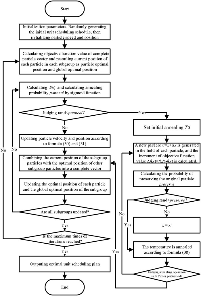
FIGURE 2. Overall flow chart of the ICPSO algorithm.

Case Study

In this study, a VPP in the coastal areas of China is taken as an example to verify the above energy management model. The VPP includes conventional generator set, distributed wind turbine, distributed photovoltaic, ESS, and flexible load. The rated capacity of the conventional generator set is 2 MW, and the minimum output of the conventional generator set is 0.5 MW. The maximum discharging power and charging power of ESS are 0.7 and 0.5 MW, respectively, and the charging and discharging efficiency is 90%. The time of use adopted in this study includes the transaction price between the VPP and the power market (market price) and the transaction price between the VPP and flexible load users (load price), as shown in Figure 3.

FIGURE 3

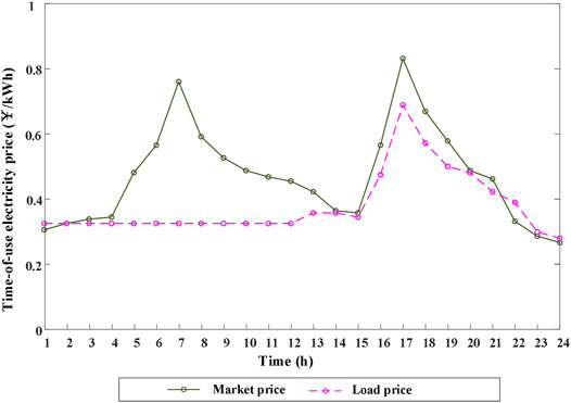
FIGURE 3. Time of use.

Both the output power of wind turbine, photovoltaic, and the flexible load power of TL, PL, and IL are shown in Figure 4.

FIGURE 4

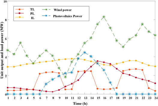
FIGURE 4. Temporal distribution of wind power output, photovoltaic power output, and flexible loads.

This case assumes that the TL non-shiftable periods T0 are 1:00–5:00 and 23: 00–24: 00. The idle periods of PL demand (the periods without requirements for indoor temperature) T1 and T2 are 9:00–12:00 and 14: 00–18: 00, respectively. The demand response periods are 6:00–8:00 and 16:00–19:00. Outdoor temperature is a typical daily temperature distribution in summer, as shown in Figure 5.

FIGURE 5

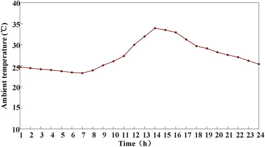
FIGURE 5. Distribution of ambient temperature.

Relevant parameter settings of the VPP energy management model are shown in Table 1.

TABLE 1

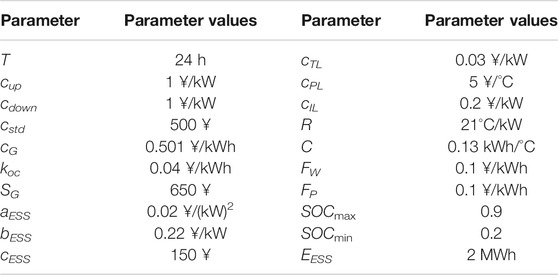
TABLE 1. Basic parameters of the proposed model.

Optimization Result Analysis

Verification of the Improved Cooperative Particle Swarm Optimization

To verify the superiority of the proposed algorithm, four typical benchmark functions (Tablet, Quadric, Griewank, and SchafferF7) were selected, and the proposed algorithm was compared with the PSO, the Genetic Algorithm (GA), and the CPSO algorithms. Among them, the first two functions are single-mode functions, and the last two functions are multi-mode functions. The expressions and variable ranges of the four functions are shown in Table 2.

TABLE 2

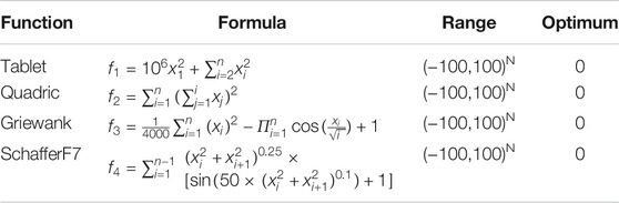
TABLE 2. Benchmark function.

The parameters of the four algorithms are set as follows: the maximum number of iterations is 100 and the number of particles is 50. Under MATLAB 2018a running environment, the ICPSO, the PSO, the GA, and the CPSO are used to run the above four functions 50 times, and the mean deviation (MD) and square deviation (SD) of the 50 times results are calculated. The results are shown in Table 3.

TABLE 3

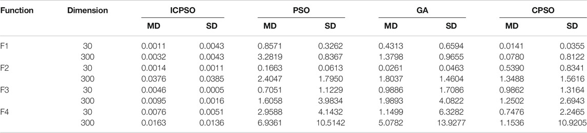
TABLE 3. Comparison results of the ICPSO, the PSO, the GA, and the CPSO algorithms.

It can be seen from Table 3 that the PSO, the GA, and the CPSO algorithms can accurately solve single-mode functions, and the CPSO algorithm is usually superior to the PSO and the GA algorithm when the particle dimension increases. When solving multimodal functions, the PSO, the GA, and the CPSO can complete the optimization, but the SD of solving such functions is too large due to the single way of updating particles. Compared with other algorithms participating in the comparison, the ICPSO algorithm proposed in this study has the best performance in solving multi-modal problems and multi-time particle dimensions.

Analysis of VPP Optimization Results Considering Flexible Load Adjustment

In order to analyze and consider the influence of flexible load adjustment on the operation of each unit in the VPP, this study calculates the optimization results of VPP energy management without considering flexible load adjustment (case1), only considering IL adjustment (case2), and considering three types of flexible load adjustment (case3), as shown in Figures 6–8.

FIGURE 6

FIGURE 6. Optimization results of case 1.

FIGURE 7

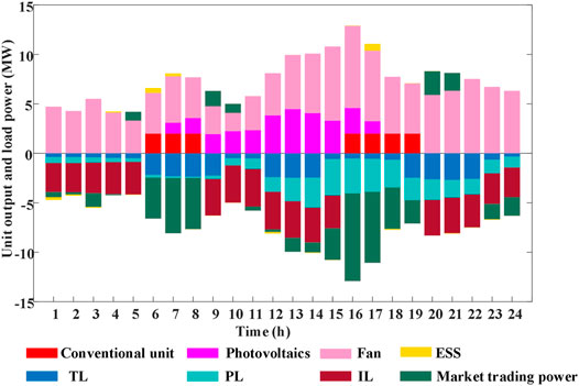
FIGURE 7. Optimization results of case 2.

FIGURE 8

FIGURE 8. Optimization results of case 3.

In Figures 6–8, the electricity quantity traded in the electricity market is greater than zero to buy electricity from the electricity market, and less than zero to sell electricity to the electricity market. ESS greater than zero indicates ESS discharging, and ESS lower than zero indicates ESS charging. Comparing Figures 6–8, it can be seen that the overall market electricity sales of case 1 is low, and according to the data calculation, the market electricity sales of case 1 is 25.10 MWh. Compared with case 1, in order to obtain higher economic benefits, case 2 and case 3 increased the market sales through load adjustment. According to the calculation, the market electricity sales in case 2 and case 3 are 47.13 MWh and 59.56 MWh, respectively, which are 22.03 MWh and 34.46 MWh higher than those in case1, and the increase is mostly concentrated in the demand response period. It should be noted that in terms of market power consumption, case 2 is 1.25 MWh less than case 1, while case 3 is 0.57 MWh more than case1. This is because in case 3, TL is shifted from the demand response period to the non-demand response period, which leads to an increase in the market purchasing power of the VPP in the non-demand response period. However, the amount of electricity purchased by the VPP in the non-demand response period has increased, resulting in a part of electricity purchase cost. The amount of electricity sold by the VPP in the demand response period will also increase correspondingly, resulting in electricity sales revenue. As this part of sales revenue can not only make up the load shift cost but also create operating income for operators, TL adjustment can bring better economic benefits to the VPP. In order to further verify the improvement of comprehensive load adjustment (case 3) on the system economy, this study calculates the relevant economic parameters in different cases and summarizes them in Table 4.

TABLE 4

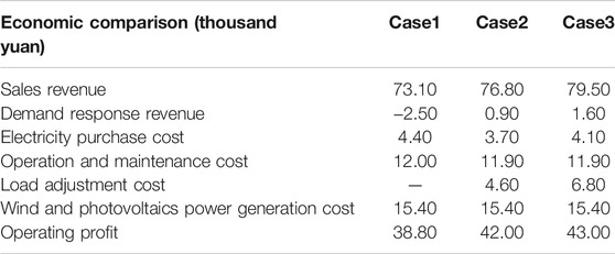
TABLE 4. Economic comparison results.

It can be seen from the economic comparison of the cases in Table 4 that although the cost of load control in case 3 is the highest, reaching 6,800 yuan, more income from electricity sales and demand response is obtained through load control. According to the calculation, the electricity sales revenue of the comprehensive load optimization control scheme proposed in this study reaches 79.50 thousand yuan, which is 8.76 and 3.52% higher than that of case1 and case 2, respectively. At the same time, the income from participating in demand response is 1.60 thousand yuan, which is 77.78% higher than that of case 2. It should be noted that the demand response income in case 1 is negative, which is due to the failure to meet the market demand response trading standards at 6:00, 8:00, 18:00, and 19:00 and the need to bear some economic penalties. In addition, the demand response income in case 2 and case 3 is far lower than the load adjustment cost, which is because the demand response income in the calculation results is only the extra income obtained according to the demand response contract and does not include the electricity price difference caused by load adjustment, which is included in the electricity sales income. Finally, the total operating profit of case 3 is 43.00 thousand yuan, which is 10.82 and 2.38% higher than that of case1 and case 2, respectively.

Influence of Electricity Marketization Trading on Flexible Load Adjustment

In order to further analyze the influence of power market transactions on flexible load adjustment, this section shows the optimization results of PL, IL, and TL adjustment, as shown in Figures 9–11.

FIGURE 9

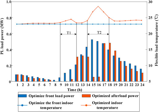
FIGURE 9. Results of PL demand and temperature change before and after optimization.

In this study, the temperature-controlled load air conditioning is taken as an example to analyze its influence on PL adjustment. It can be seen from Figure 9 that before optimization, in order to ensure that the indoor temperature is always below the expected value, the equipment needs continuous power supply, resulting in large power consumption when the outdoor temperature is high from 9:00 to 18:00. Since T1 period and T2 period are idle periods for PL demand of users, there is no strict demand for indoor temperature at this time, so the practice of keeping constant temperature will lead to partial waste of electric energy. By implementing the optimization method proposed in this study, PL can reduce the operating power in T1 period and T2 period. At the same time, before the end of T1 period and T2 period, the flexible temperature control load is turned on in advance to reduce the indoor temperature, so that the temperature can be kept within the comfort range of the human body during the normal demand period. According to the numerical calculation, in this optimization, PL-based adjustment reduced the electricity consumption by 10.36 MWh, saved the users electricity cost by 3.80 thousand yuan, and got the electricity-saving subsidy of 1.90 thousand yuan. In addition, it should be noted that in Figure 9, there is a significant difference in the rising amplitude of indoor temperature between T1 period and T2 period. This is because the outdoor temperature rises slightly during T1 period, and the indoor temperature rises slightly in order to reduce part of the load. At T2 period, the outdoor temperature reaches a high level, and the indoor temperature will increase greatly in order to reduce the load.

The above results show that the implementation of PL adjustment can greatly reduce PL users’ electricity consumption during the demand response period and the demand idle period without significantly affecting users’ comfort and reduce their electricity purchase cost.

It can be seen from Figure 10 that according to the IL adjustment strategy in this study, IL is completely interrupted during the demand response period. Combined with Table 4, it is calculated that compared with the situation without IL adjustment, the implementation of IL adjustment can increase the income from VPP sales by 3.70 thousand yuan, the income from demand response by 3.40 thousand yuan, and the overall income by 3.20 thousand yuan. However, the implementation of IL adjustment needs to pay an additional subsidy of 4.60 thousand yuan for user comfort loss.

FIGURE 10

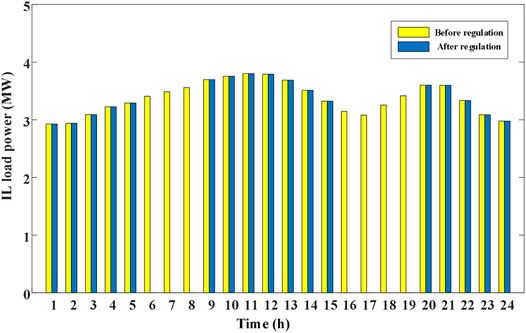
FIGURE 10. Time-by-time distribution of IL demand before and after optimization.

The above results show that the implementation of IL adjustment is helpful to improve users’ electricity consumption economy and VPP overall income. However, compared with PL adjustment, IL adjustment has a more obvious impact on users’ comfort by greatly reducing the load of users’ demand response period.

It can be seen from Figure 11 that similar to IL, in order to obtain demand response revenue, the VPP cuts TL during the demand response period. In addition, TL is increased in the non-demand response period at 10:00, 11:00, etc. The above load shift can provide more trading power for the VPP to participate in power grid interaction. According to the data calculation, the total load shift of case3 throughout the day is 7.77 MWh. In addition, load shift-in mainly occurs in the PL demand idle period, and the shift-in amount in this period accounts for 90.07% of all-day shift-in. This situation shows that the optimization method proposed in this study can compensate for the load fluctuation caused by PL reduction through TL shifts.

FIGURE 11

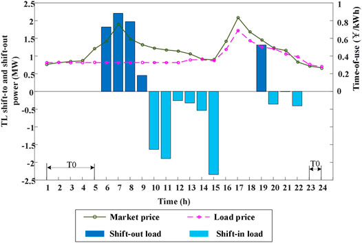
FIGURE 11. Time-by-time distribution of TL shift-in/shift-out quantity.

The above results show that TL adjustment can further improve the load reduction of the VPP in the demand response period and at the same time compensate for the load fluctuation caused by PL adjustment to a certain extent, thus forming collaborative scheduling among different types of flexible loads. In addition, TL adjustment does not significantly affect user comfort.

Conclusion

A VPP is a typical form of collaborative optimization of distributed generation resources, adjustable loads, and energy storage equipment, which plays an important role in improving the efficiency of energy management on the demand side. In this study, based on the existing research on energy management of VPPs, the cost of flexible load adjustment is included in the objective function, and the energy management model of the VPP is constructed. Then the ICPSO is used to solve the output, flexible load control, and energy storage charging and discharging plan of each unit in the VPP. Finally, the optimization results are compared and analyzed in different scenarios. The case analysis results show that compared with other algorithms, the ICPSO algorithm proposed in this study has the best performance in solving multi-modal problems and multi-particle dimension problems. The VPP energy management model proposed in this study has improved operating profit by 10.82 and 2.38%, respectively, compared with the optimization scheme without considering flexible load adjustment and only considering IL adjustment.

With the further opening of the electricity market, distributed generation equipment and flexible load users will freely choose the VPP according to their own interests, and the VPP structure will be changed from the fixed structure in this study to the dynamic structure. In addition, the unit price of user comfort allowance considered in this study only represents the current living standard of residents. With the development of society and economy, the improvement of people’s living standard will further change the unit price of user comfort allowance. Therefore, how to realize the dynamic matching between distributed generation equipment, flexible load users, and VPPs and accurately analyze the impact of the improvement of flexible load users’ living standards on VPP energy management are the problems to be solved in the future.

Data Availability Statement

The original contributions presented in the study are included in the article/Supplementary Material, further inquiries can be directed to the corresponding author.

Author Contributions

DY, XZ, YW, LJ, and HL: conceptualization, data curation, writing—original draft, and writing—review and editing.

Funding

This research was funded by the National Science Foundation China “Research on Theory and Method of Userside Integrated Energy Optimization Based on Multi-Agent Game” (No. U1766210).

Conflict of Interest

The authors declare that the research was conducted in the absence of any commercial or financial relationships that could be construed as a potential conflict of interest.

Publisher’s Note

All claims expressed in this article are solely those of the authors and do not necessarily represent those of their affiliated organizations, or those of the publisher, the editors, and the reviewers. Any product that may be evaluated in this article, or claim that may be made by its manufacturer, is not guaranteed or endorsed by the publisher.

Acknowledgments

We gracefully acknowledge the Beijing Key Laboratory of Demand Side Multi-Energy Carriers Optimization and Interaction Technique for its invaluable contributions during this collaboration.

References

Azizivahed, A., Naderi, E., Narimani, H., Fathi, M., and Narimani, M. R. (2017). A New Bi-objective Approach to Energy Management in Distribution Networks with Energy Storage Systems. IEEE Trans. Sustain. Energ. 9(1), 56–64. doi:10.1109/tste.2017.2714644

CrossRef Full Text | Google Scholar

Babaee Tirkolaee, E., Goli, A., and Weber, G.-W. (2020). Fuzzy Mathematical Programming and Self-Adaptive Artificial Fish Swarm Algorithm for Just-In-Time Energy-Aware Flow Shop Scheduling Problem with Outsourcing Option. IEEE Trans. Fuzzy Syst. 28 (11), 2772–2783. doi:10.1109/tfuzz.2020.2998174

CrossRef Full Text | Google Scholar

Baringo, A., Baringo, L., and Arroyo, J. M. (2019). Day-Ahead Self-Scheduling of a Virtual Power Plant in Energy and Reserve Electricity Markets under Uncertainty. IEEE Trans. Power Syst. 34 (3), 1881–1894. doi:10.1109/tpwrs.2018.2883753

CrossRef Full Text | Google Scholar

Charalampakis, A. E., and Tsiatas, G. C. (2019). Critical Evaluation of Metaheuristic Algorithms for Weight Minimization of Truss Structures. Front. Built Environ. 5 (113), 1–17. doi:10.3389/fbuil.2019.00113

PubMed Abstract | CrossRef Full Text | Google Scholar

Dilantha, H., Daswin, D. S., and Seppo, S. (2021). Solar Irradiance Nowcasting for Virtual Power Plants Using Multimodal Long Short-Term Memory Networks. Front. Energ. Res. (9) doi:10.3389/fenrg.2021.722212

CrossRef Full Text | Google Scholar

Elmorshedy, M. F., Elkadeem, M. R., Kotb, K. M., Taha, I. B. M., and Domenico, M. (2021). Optimal Design and Energy Management of an Isolated Fully Renewable Energy System Integrating Batteries and Supercapacitors. Energ. Convers. Manage. 245, 114584. doi:10.1016/j.enconman.2021.114584

CrossRef Full Text | Google Scholar

Faa-Jeng Lin, F. J., Li-Tao Teng, L. T., Jeng-Wen Lin, J. W., and Syuan-Yi Chen, S. Y. (2009). Recurrent Functional-Link-Based Fuzzy-Neural-Network-Controlled Induction-Generator System Using Improved Particle Swarm Optimization. IEEE Trans. Ind. Electron. 56 (5), 1557–1577. doi:10.1109/tie.2008.2010105

CrossRef Full Text | Google Scholar

Hannan, M. A., Al-Shetwi, A. Q., Ker, P. J., Begum, R. A., Mansor, M., Rahman, S. A., et al. (2021). Impact of Renewable Energy Utilization and Artificial Intelligence in Achieving Sustainable Development Goals. Energ. Rep. 7, 5359–5373. doi:10.1016/j.egyr.2021.08.172

CrossRef Full Text | Google Scholar

Li, J. M., Ai, Q., and Yin, S. R. (2021). Market Mechanism of Virtual Power Plant Participating in Peak Shaving and Frequency Modulation Service and Foreign Experience for Reference. J. Chin. Electr. Eng., 1–21. doi:10.13334/j.0258-8013.pcsee.202152

CrossRef Full Text | Google Scholar

Liang, D., Zhan, Z.-H., Zhang, Y., and Zhang, J. (2020). An Efficient Ant Colony System Approach for New Energy Vehicle Dispatch Problem. IEEE Trans. Intell. Transport. Syst. 21 (11), 4784–4797. doi:10.1109/tits.2019.2946711

CrossRef Full Text | Google Scholar

Lu, C. Y. (2021). Quantitative Analysis of Distributed Dispatch and Cost Planning of Shared Cars Based on Simulated Annealing Algorithm. Scientific J. Econ. Manage. Res. 3 (5), 316–328. doi:10.13334/j.0258-8013.pcsee.202152

CrossRef Full Text | Google Scholar

Luo, F. Z., Yang, X., Wei, W., Zhang, T. Y., Yao, L. Z., Zhu, L. Z., et al. (2020). Bi-Level Load Peak Shifting and Valley Filling Dispatch Model of Distribution Systems with Virtual Power Plants. Front. Energ. Res. 8. doi:10.3389/fenrg.2020.596817

CrossRef Full Text | Google Scholar

Mears, A., and Martin, J. (2020). Fully Flexible Loads in Distributed Energy Management: PV, Batteries, Loads, and Value Stacking in Virtual Power Plants. Engineering 6 (7), 736–738. doi:10.1016/j.eng.2020.07.004

CrossRef Full Text | Google Scholar

Mellouk, L., Ghazi, M., Aaroud, A., Boulmalf, M., Benhaddou, D., and Zine-Dine., (2019). Design and Energy Management Optimization for Hybrid Renewable Energy System- Case Study: Laayoune Region. Renew. Energ. 139, 621–634. doi:10.1016/j.renene.2019.02.066

CrossRef Full Text | Google Scholar

Mohammad, J. K., Majid, G., and Javad, N. (2017). Optimal Management of Renewable Energy Sources by Virtual Power Plant. Renew. Energ. 114, 1180–1188. doi:10.1016/j.renene.2017.08.010

CrossRef Full Text | Google Scholar

Naughton, J., Wang, H., Cantoni, M., and Mancarella, P. (2021). Co-Optimizing Virtual Power Plant Services under Uncertainty: A Robust Scheduling and Receding Horizon Dispatch Approach. IEEE Trans. Power Syst. 36 (5), 3960–3972. doi:10.1109/tpwrs.2021.3062582

CrossRef Full Text | Google Scholar

Qu, X. Y., Hui, H. X., Yang, S. C., Li, Y. P., and Ding, Y. (2018). Price Elasticity Matrix of Demand in Power System Considering Demand Response Programs. IOP Conf. Ser. Earth Environ. Sci. 121 (5).052081. doi:10.1088/1755-1315/121/5/052081

CrossRef Full Text | Google Scholar

Riget, J., and Vesterstrøm, J. S. (2002). A Diversity-Guided Particle Swarm Optimizer – the ARPSO. Aarhus: dept.comput.sci.univ.of aarhus.

Google Scholar

Shabani, H. R., and Kalantar, M. (2021). Real-time Transient Stability Detection in the Power System with High Penetration of DFIG-Based Wind Farms Using Transient Energy Function. Int. J. Electr. Power Energ. Syst., 133, 107319. doi:10.1016/j.ijepes.2021.107319

CrossRef Full Text | Google Scholar

Tan, C. X., Wang, J., Geng, S. P., Pu, L., and Tan, Z. F. (2021). Three-level Market Optimization Model of Virtual Power Plant with Carbon Capture Equipment Considering Copula–CVaR Theory. Energy 237, 121620. doi:10.1016/j.energy.2021.121620

CrossRef Full Text | Google Scholar

vandenBergh, F., and Engelbrecht, A. P. (2004). A Cooperative Approach to Particle Swarm Optimization. IEEE Trans. Evol. Computat. 8 (3), 225–239. doi:10.1109/tevc.2004.826069

CrossRef Full Text | Google Scholar

Vohra, V., and Sano, T. (2021). Colorless Windows that Transform Sunlight into Electricity. Front. Young Minds 9, 552439. doi:10.3389/frym.2021.552439

CrossRef Full Text | Google Scholar

Wang, K. K., Nan, D. L., Li, Y., Zhang, L., and Li, X. Z. (2020). Double-layer Optimal Operation Strategy of Virtual Power Plant Participating in Large-Scale New Energy System on Energy Storage Side. J. Chin. Electr. Eng. 15 (02), 24–33.

Google Scholar

Yang, J. B., Xu, X. H., Peng, Y. Q., Zhang, J. Y., and Song, P. Y. (2019). Modeling and Optimal Energy Management Strategy for a Catenary-Battery-Ultracapacitor Based Hybrid Tramway. Energy 183, 1123–1135. doi:10.1016/j.energy.2019.07.010

CrossRef Full Text | Google Scholar

Yang, S. X., Zhu, X. G., and Peng, S. J. (2020). Prospect Prediction of Terminal Clean Power Consumption in China via LSSVM Algorithm Based on Improved Evolutionary Game Theory. Energies 13 (8), 2065. doi:10.3390/en13082065

CrossRef Full Text | Google Scholar

Yoon, J. H., Baldick, R., and Novoselac, A. (2014). Dynamic Demand Response Controller Based on Real-Time Retail Price for Residential Buildings. IEEE Trans. Smart Grid 5 (1), 121–129. doi:10.1109/TSG.2013.2264970

CrossRef Full Text | Google Scholar

Yu, D. M., Liu, H. N., and Bresser, C. (2018). Peak Load Management Based on Hybrid Power Generation and Demand Response. Energy 163, 969–985. doi:10.1016/j.energy.2018.08.177

CrossRef Full Text | Google Scholar

Yu, D., Zhu, H., Han, W., and Holburn, D. (2019). Dynamic Multi Agent-Based Management and Load Frequency Control of PV/Fuel Cell/Wind Turbine/CHP in Autonomous Microgrid System. Energy 173, 554–568. doi:10.1016/j.energy.2019.02.094

CrossRef Full Text | Google Scholar

Zhang, K. Q., Qu, Z. X., Dong, Y. X., Lu, H. Y., Leng, W. N., and Wang, J. Z. (2019). Research on a Combined Model Based on Linear and Nonlinear Features - A Case Study of Wind Speed Forecasting. Renew. Energ. 130, 814–830. doi:10.1016/j.renene.2018.05.093

CrossRef Full Text | Google Scholar

Zhang, T., Ma, J. H., Yan, X., Huang, W. R., Wang, L., Xu, S. Q., et al. (2021). Strategy Optimization for Virtual Power Plant Complied with Power to Gas Operation Model. J. Phys. Conf. Ser. 2005 (1).012146. doi:10.1088/1742-6596/2005/1/012146

CrossRef Full Text | Google Scholar

Zhao, B., Wang, X., Lin, D., Calvin, M. M., Morgan, J. C., Qin, R., et al. (2018). Energy Management of Multiple Microgrids Based on a System of Systems Architecture. IEEE Trans. Power Syst. 33 (6), 6410–6421. doi:10.1109/tpwrs.2018.2840055

CrossRef Full Text | Google Scholar

Zhu, J., Lauri, F., Koukam, A., and Hilaire, V. (2015). Scheduling Optimization of Smart Homes Based on Demand Response[C]//IFIP International Conference on Artificial Intelligence Applications and Innovations. Cham: Springer.

Google Scholar

Zhu, J. W., Lin, Y. H., Lei, W. D., Liu, Y. Q., and Tao, M. L. (2019). Optimal Household Appliances Scheduling of Multiple Smart Homes Using an Improved Cooperative Algorithm. Energy 171, 944955. doi:10.1016/j.energy.2019.01.025

CrossRef Full Text | Google Scholar