 Zhentao Han1
 Hao Lu
 Siyu Xu
 Weiye Zheng
- 1State Grid Liaoning Electric Power Company Limited, Economic Research Institute, Shenyang, China
- 2State Grid Liaoning Electric Power Supply Co., LTD., Shenyang, China
- 3School of Electrical Power Engineering, South China University of Technology, Guangzhou, China
The rapid growth of distributed generation (DG) and load has highlighted the necessity of optimizing their ways of integration, as their siting and sizing significantly impact distribution networks. However, little attention has been paid to the siting and sizing of new substations which are to be installed. This paper proposes deep learning-aided joint DG-substation siting and sizing in distribution network stochastic expansion planning. First, as the model depends on an accurate forecast, Long Short-Term Memory (LSTM) deep neural network is used to forecast DG output and load, where electricity growth rate, bidding capacity of the electric expansion, and industrial difference are all considered. Then, a two-stage stochastic mixed integer bilinear programming model was established for joint DG-substation siting and sizing under uncertainties, where multiple objective functions are comprehensively addressed. By using the Fortuny-Amat McCarl Linearization, the resultant bilinear model is equivalently transformed into a mixed integer linear program, which can be efficiently solved. Finally, stochastic power flow calculation in the IEEE 69-node system is conducted to analyze the influence of electric expansion and DG integration on the node voltage and power flow distribution of the power system. The effectiveness of the proposed method is also verified by simulation tests.
1 Introduction
With the forthcoming shortage of fossil fuels, the accommodation of renewable energy is a critical topic in power systems. Although large-scale integration of DGs is favorable to promoting the development of the economy, environment, and society (Singh and Sharma, 2017), curtailment of renewable energy is still significant and remains a critical issue to date (Zheng et al., 2021; Zheng et al., 2022). On the other hand, the expansion capacity of different industries will also impact the demand side of the system. It is left open how to reasonably plan the location and capacity of the renewables and the expanded industrial load to be integrated into the system, as the planning scheme has a huge impact on the operation of the power system.
Load forecasting and DG forecasting are important basis for power system decision-making and planning. In terms of load forecasting, due to the volatility of DG and load, how to accurately forecast the load in the presence of electric expansion is the focus of this research. The existing load forecasting research is mainly divided into statistics-based and learning-based methods, and the latter is the current mainstream method. Statistical methods mainly include multiple linear regression, autoregression, autoregressive moving average, and so on (Kim et al., 2018; Ahmad and Chen, 2019), but they can hardly deal with load data with random and dynamic development. (Yang et al., 2019). establishes a hybrid power load forecasting model by combining the autocorrelation function and least squares support vector machine in short-term power load forecasting. Compared with the benchmark model, experimental results show that this method can significantly improve forecasting accuracy. (Gul et al., 2021). adopts CNN-Bi-LSTM to process time series data sets for medium-term electricity prediction. However, the industrial difference in electricity consumption needs to be studied, while the quantitative relationship between industrial expansion capacity and the growth of load needs to be revealed. In this paper, the influence of industrial expansion will be considered in load forecasting, while the influence of direct irradiance and diffuse irradiance will be considered in DG sizing forecasting.
Although pioneering studies have investigated the siting and sizing of DG in the distribution network, little attention has been paid to installing new substations for industrial expansion. (Ho et al., 2016). proposes an optimal energy storage scheduling of DG distributed power generation system, which was formulated as a mixed integer linear program (MILP). (Vale et al., 2010). adopts the artificial neural network method to carry out distributed energy scheduling in isolated grids, and the construction of virtual power participants (VPP) can aggregate large-scale integration of DG and other distributed energy resources. (Daud et al., 2016). studies how to deploy the optimal location capacity of distributed photovoltaics. This paper considers multiple objectives such as power loss, voltage deviation, average voltage total harmonic distortion, and system average voltage decline to construct a multi-objective optimization problem, and the multi-objective optimization problem is converted into a single-objective optimization problem in a weighted way. In the research on industrial expansion, (Chen and Hsu, 1989). establishes an expert system for load allocation in the industrial expansion planning of the distribution network. The artificial language PROLOG is used to integrate the heuristic rules followed by the load allocation planner into the knowledge base, generating several appropriate load distribution schemes. (Aghaei et al., 2014). proposes a multi-stage distribution network expansion planning algorithm based on improved particle swarm optimization to ensure energy reliability and security, and realize the integration of distributed generation units into the distribution network. (Fan et al., 2020). considers the uncertainties of DG and electric vehicles and develops a comprehensive extended programming framework based on multi-objective mixed integer non-linear programming, where the Chebyshev decomposition is employed to solve the problem. However, heuristic algorithms can barely consider the uncertainty of DG and load, and their computational efficiency is generally low, which cannot satisfy the need for real-time dispatch.
Compared with the existing research on the siting and sizing of DGs, this paper tackles the scenario with industrial expansion by using the research framework in Figure 1. Utility companies process customers’ applications for new substation installation and additional electricity capacity, referred to as industrial expansion and installation. Meanwhile, the main ways to achieve capacity growth include the installation of DG and substation. Therefore, this paper further explores the problem of joint DG-substation siting and sizing. The contributions are three-fold:
1) Industrial expansion data are fully employed in the LSTM network to forecast the increment load brought by the expansion.
2) A two-stage stochastic optimization model for joint DG-substation siting and sizing is established, which is reformulated into a mixed-integer linear program for an efficient solution.
3) Simulation tests are conducted on an IEEE system to prove the effectiveness of the research. Stochastic power flow is carried out to evaluate the impact of DG/substation integration on the system states, highlighting the merits of joint DG-substation siting and sizing.
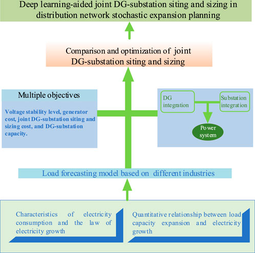
FIGURE 1. The research framework of this paper.
Deep learning-based load forecasting and DG capacity forecasting
Load forecasting considering industrial expansion
As the industrial load is affected by industrial expansion and seasonal fluctuations, this paper improves the traditional LSTM load forecasting network, and applies the data of industrial expansion and electricity growth of different industries to the neural network, to more accurately forecast the load level under the influence of industrial expansion (Zheng et al., 2020).
In this section, the monthly load data of the pharmaceutical manufacturing industry, rubber and plastic products industry, and transportation, electrical and electronic equipment manufacturing industry in a province under the influence of industrial expansion are used to build an LSTM network, providing a basis for the load growth generated by industry expansion business.
The constructed model consists of the following steps:
1) Data selection
A large number of industrial expansion data are screened to eliminate the data caused by fault maintenance and line change and to ensure that the analyzed industrial expansion capacity generates actual load.
2) Data pre-processing
Assuming that the current time period is t, we select the industry monthly load data, annual load growth rate, and industrial expansion capacity of the past d time period for normalization and use them as the input of LSTM.
3) LSTM network structure
As shown in Figure 2, the network consists of an input layer, H sequence blocks, and an output layer. Firstly, the input layer is used to preprocess the load data, then the sequence blocks constructed by H custom LSTMs are used to extract the features of the input sequence, and finally, the output layer generates the load forecast for the industry.
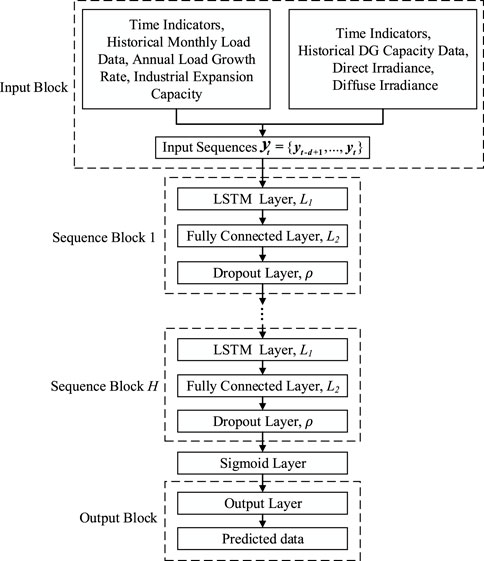
FIGURE 2. LSTM network structure diagram.
Each sequence block has the same structure, including an LSTM layer, a fully connected layer, and a dropout layer. LSTM network is a recurrent neural network that can establish the temporal correlation between previous information and the current environment, so LSTM is used as a basic component of sequence blocks. Each LSTM layer L1 has multiple units, each of which has a memory unit
Where
The input node, input gate, forgetting gate, and output gate are shown in Eq. 1–4. Different activation functions are used to calculate the activation of the weighted sum of input
4) The setting of training parameters
In the above network structure, each Bernoulli random variable has probability
Finally, in the training of the network, the time algorithm is used for back-propagation (Gers et al., 1999) to minimize the loss between the predicted output of the neural network
The historical data of training is input into the above network, and the predicted load value of the current time period
DG capacity forecasting
Given that the output of DG is affected by some factors, such as environment, time, and so on, this section similarly uses the LSTM network to learn the historical data output by DG to predict the output capacity of DG more accurately. Therefore, as shown in Figure 2, the DG capacity data, direct irradiance, and diffuse irradiance of the same period in the province are selected for normalization and used as the input of LSTM. The network structure and training process are the same as in the previous section, and finally, the DG output data at this moment is obtained.
A multi-objective two-stage stochastic optimization model for joint DG-substation siting and sizing
The previous section forecasts the load yielded by industrial expansion and DG output, which provides the data basis for the modeling in this section. This section will use multi-objective two-stage stochastic programming to deal with the uncertainties of DGs and loads, which will be reformulated into an MILP for an efficient solution.
Objective function
A multi-objective two-stage stochastic optimization model is established. The system voltage stability and generator cost are considered in the objective function. The location and capacity of new DGs and substations are formulated as the first-stage variables, and the other variables are the second-stage variables:
where s is the number of scenarios, ωs is the probability of scenario s, and Nbus is the number of nodes in the system, Ns is the number of scenarios. Ui,s is the square of the voltage amplitude of node i in scenario s. Ng is the number of generators in the system, PGi,s is the output of the ith generator in scenario s, CGi is the cost coefficient of the ith generator. Next is the number of substation installation,
The original problem can be transformed into a single-objective optimization problem by weighting the multi-objective, which can be directly solved by the mainstream solver. Therefore, this paper converts the above multi-objective optimization problem into the following single-objective optimization problem:
In Eq. 11,
Network constraint
Since the joint DG-substation siting and sizing are usually in the distribution network, considering the distribution network is a radial network, LinDistFlow model is used to describe the power flow (Šulc et al., 2014):
Among them, Equations 12, 13 are the active and reactive power balance constraints of node i, Pji,s/Qji,s is the active and reactive power flow between nodes j and i in scenario s, PDG,i,s/QDG,i,s is the active and reactive power capacity of DG integration at node i in scenario s. Pdi/Qdi is the active/reactive power load of node i,
In scenario s, the additional load at node i is shown in Eqs 21, 22.
In scenario s, the capacity of DG integrated at node i is shown in Eqs 23, 24.
Among all variables, αki, βki are the first-stage variables, Ui,s, PGi,s, Pji,s/Qji,s, Pdi/Qdi, PDG,i,s/QDG,i,s,
Among them, constraints (25), (27), (29) and (31) are to deal with the non-linearity arising from the multiplication of binary variables and continuous variables in Eq. 21, and constraints (26), (28), (30) and (32) are to deal with the non-linear problem in Eq. 23, and the parameter M is set to a large number.
Finally, our final model using Fortuny-Amat McCarl Linearization is as follows:
Constraints include Eqs. 12-32. The reformulated problem is an MILP.
Case study
Case studies are conducted on the IEEE 69-node system. The deep learning part is implemented by using tensorflow 1.14.0. The MILP model is established by Yalmip, and solved by the commercial solver Gurobi. In this section, firstly, stochastic power flow is used to measure the impact of DG-substation siting and sizing on the distribution network, highlighting the merits of this research. Then, the accuracy of the load forecast under industrial expansion is tested. Finally, based on two-stage stochastic programming, the optimization results of joint DG-substation siting and sizing are analyzed.
Impact of DG-substation siting on the distribution network under uncertainties
In this paper, the Monte Carlo method is used to measure the impact of DG integration on the distribution system. Firstly, it generated several groups of data through the probability distribution of DG integration to reflect the uncertainty of DG, then used these data to carry out Monte Carlo stochastic power flow simulation respectively. Finally, it statistically analyzed the voltage probability distribution of four typical nodes, node 2, node 26, node 53, and node 68, and analyzed the results. The sample size of the Monte Carlo simulation is set to 1000, the fluctuation of DG integration is set to the Gaussian distribution of mathematical expectation is
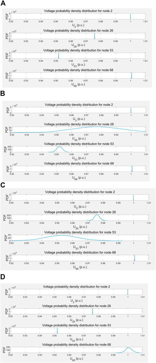
FIGURE 3. Voltage probability distribution of four typical nodes: (A) the DG is connected to node 3, (B) the DG is connected to node 25, (C) the DG is connected to node 52, (D) the DG is connected to node 67.
The simulation results are shown in Figures 3A–D, whose scenarios are explained as follows. Figure 3A: When DG is connected to node 3, there is no voltage fluctuation everywhere. Figure 3B: When DG is connected to node 25, the voltage fluctuation of node 26 is relatively obvious, the voltage of node 53 fluctuates slightly, and the voltage of the other two places has no fluctuation. Figure 3C: When DG is connected to node 52, the voltage fluctuation of node 53 is relatively significant, the voltage of node 26 fluctuates slightly, and the voltage of the other two places has no fluctuation. Figure 3D: When DG is connected to node 67, the voltage at node 68 fluctuates slightly, while the voltage at other places does not fluctuate.
The sensitivity of each node to DG integration is different. Because the location of node 2 is very close to the root node, the voltage of node 2 is almost not affected by the location of DG. The locations of nodes 26, 53, and 68 are all at the end of their branches, and their voltages are greatly affected by the location of DG.
Different locations of DG integration have different effects on the voltage of each node in the system. It can be seen from Figures 3B–D that when the DG integration causes the voltage fluctuation of a node, the voltage of the node closer to the node will be more affected by it. Therefore, the DG is connected to a location far away from the important load, which can reduce the adverse impact on the voltage of the important load.
The amplitude of node voltage fluctuation is significantly affected by the branch impedance sum of the branch where the node is located. Due to the small sum of branch impedances of node 68, the voltage in Figures 3A–C is not affected by the integration to DG basically, and it is also less affected by the integration to DG in Figure 3D. The voltage of node 26 and node 53 have obvious fluctuations when the DG is connected to node 25 (Figure 3B) and node 52 (Figure 3C), respectively. Therefore, DG is connected to the branch impedance and the small branch, which can maximize the absorption of DG.
Load forecasting and DG capacity forecasting results
In load forecasting, this paper chooses a province pharmaceutical manufacturing industry, rubber and plastic products industry, and transportation, electrical and electronic equipment manufacturing industry for 3 months in load data, load growth, industry reporting for expanding capacity, and load time series as input of LSTM, as shown in Figure 4. The detailed data are available in (Han et al., 2022).
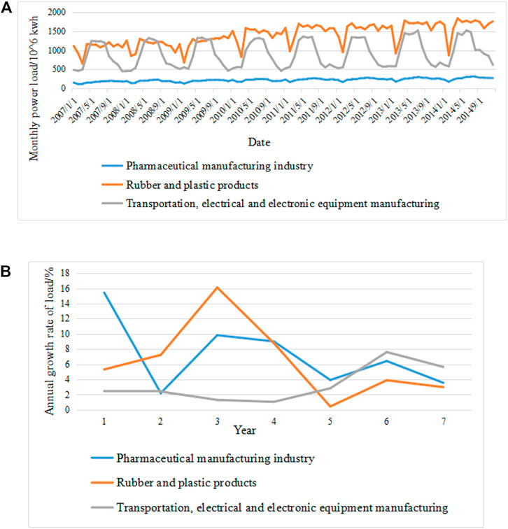
FIGURE 4. The input of LSTM: (A) monthly load curves for three industries, (B) Annual load growth curves for three industries.
Taking the pharmaceutical manufacturing industry as an example, the training loss function curve is shown in Figure 5A. It can be seen that the loss value of the training set is reduced from 0.20 to 0.00045, the loss value of the validation set is reduced from 0.175 to 0.00032, and the iteration can converge.
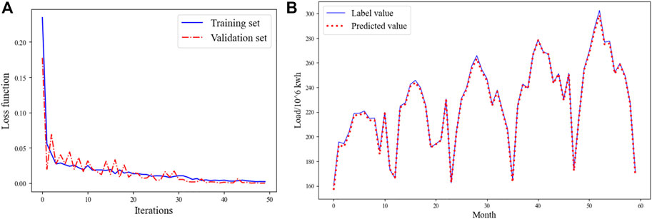
FIGURE 5. The result of pharmaceutical manufacturing industry load forecasting: (A) loss function curve, (B) comparison curve between the predicted value and the label value.
Further, the model is used to generate the predicted value of the test set and compare it with the actual label value, as shown in Figure 5B. The average absolute error of the statistical data is 782.2870.
Finally, the average relative percentage error of the predicted value of the three industry loads is no more than 2.9820%, and the error value is no more than 10%, which means the accuracy meets the system’s requirements.
In the prediction of DG capacity, the historical DG capacity data, direct irradiance, and diffuse irradiance of the same period are selected for normalization and used as the input of LSTM as shown in Figure 6. Since the historical data of the DG capacity, direct irradiance and diffuse irradiance in the IEEE 69-node system are not available, we use the real data from the platform Open Power System Data (Open Power System). The data in France in a period of 96 months from Jan. 2007 to Dec. 2014 are used, for their data integrity is relatively better. The loss function curve of DG capacity data forecasting is shown in Figure 7A, while the comparison curve between the predicted value and the label value is shown in Figure 7B. Their average relative error does not exceed 0.5451%, which is acceptable.
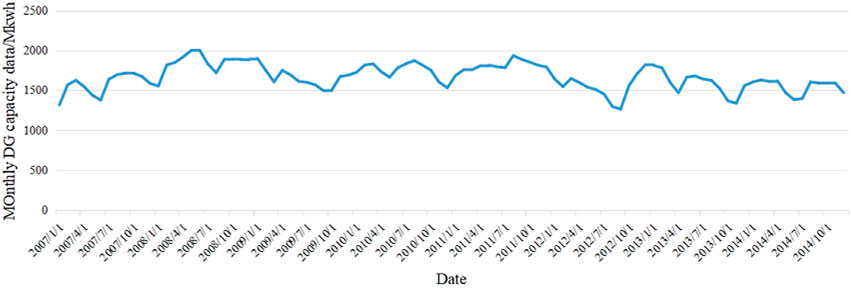
FIGURE 6. Monthly DG capacity data curve.
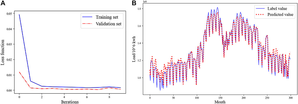
FIGURE 7. The result of DG capacity data forecasting: (A) loss function curve, (B) comparison curve between the predicted value and the label value.
Analysis of joint DG-substation siting and sizing
The load forecasting and DG capacity forecasting results obtained in the previous section under different scenarios are normalized. In order to consider the error of the forecasting results, Gaussian distribution error is added to the forecasting results, and k-means algorithm is used to generate the load and DG capacity of three groups of typical scenarios and the probability of the scenario. The load and DG capacity of the three sets of scenarios are taken as the input of the substation and DG integration model and are denoted as the maximum value of the system. It can be known that there are three joint DG-substation siting and sizing tasks, and at the same time, two DG integration tasks are set with the same probability to optimize the joint DG-substation siting and sizing.
In order to test the effect of comprehensive consideration of the multi-objective of the proposed method,
TABLE 1. Multi-objective optimization of joint DG-substation siting and sizing.
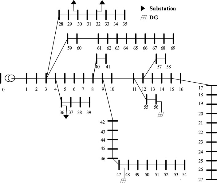
FIGURE 8. Optimal sites of DG and substation based on multiple objective optimization.
Figure 9 shows the influence of whether the objective function f1 is considered on the voltage of each node in the system in scenario 1. It can be seen that when f1 is not considered, many nodes deviate from the rated voltage significantly. However, after considering the objective function f1, the node voltage level of the system is significantly improved.
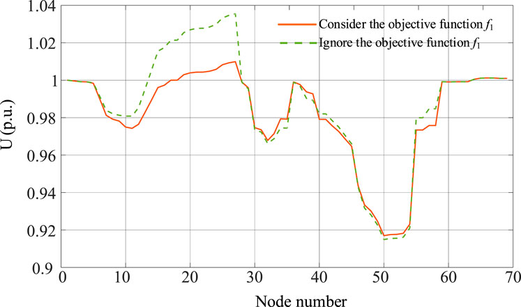
FIGURE 9. Squared node voltage in scenario one based on multiple objective optimization.
To verify the effectiveness of joint DG-substation siting and sizing, we set the control group which only considers DG siting and sizing, a total of three groups are compared, and the obtained optimization results are shown in Table 2.
1) Joint DG-substation: joint DG-substation siting and sizing are optimized.
2) Method 1: The location of the substation is fixed and the capacity is optimized, and DG siting and sizing are optimized.
3) Method 2: The location of the substation is fixed and the capacity is fixed, and DG siting and sizing are optimized.
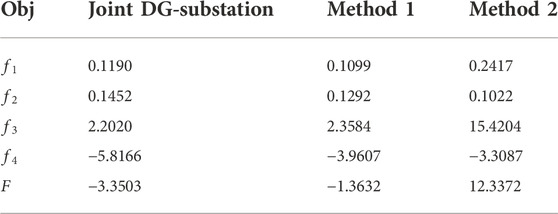
TABLE 2. Comparison of objective function values between the proposed joint DG-substation optimization and other methods.
It can be found that the voltage stability level of the system f1 and the generator cost f2 are not far apart in method 1 and joint DG-substation, but in method 2, the voltage stability level of the system f1 is relatively worse. However, the integration cost f3 is less in the case of joint DG-substation, and the expansion capacity f4 is larger, so the total objective function value is smaller in the end.
Further, 300 scenarios under four different weights
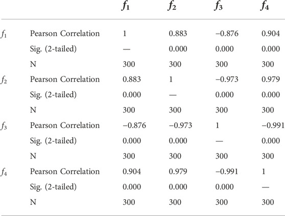
TABLE 3. Correlation analysis of the objective function in weight

TABLE 4. Correlation analysis of the objective function in weight
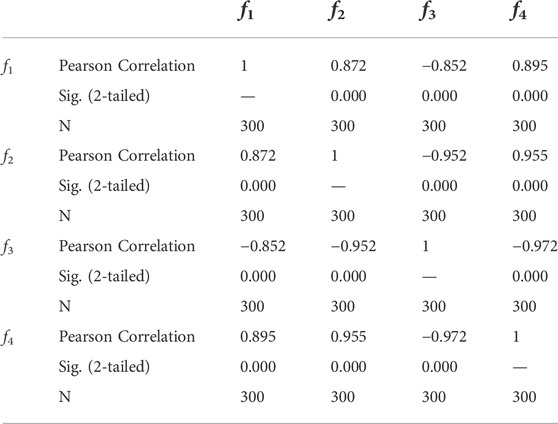
TABLE 5. Correlation analysis of the objective function in weight
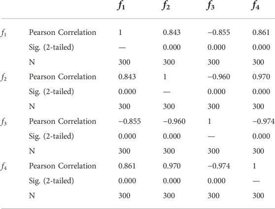
TABLE 6. Correlation analysis of the objective function in weight
Therefore, the scheme of joint DG-substation siting and sizing determined by this method can make the power flow distribution of the distribution network reasonable and the voltage level close to the rated voltage by optimizing the integration location, and also reduce the system operation cost and the joint DG-substation siting and sizing cost to some extent.
Conclusion
To answer the call of industrial expansion, this paper proposes deep learning-aided joint DG-substation siting and sizing in distribution network stochastic expansion planning. Industrial expansion data are fully employed in the LSTM network to forecast the increment load brought by the expansion. A two-stage stochastic optimization model for joint DG-substation siting and sizing is established, which is reformulated into a mixed-integer linear program for an efficient solution. Simulation tests are conducted on an IEEE system to prove the effectiveness of the research. Stochastic power flow is carried out to evaluate the impact of DG/substation integration on the system states, highlighting the merits of joint DG-substation siting and sizing. Case studies show that the forecasting results meet the accuracy requirements, and the proposed siting and sizing method is computationally efficient. It can reduce the total cost of system operation as well as alleviate the system voltage fluctuation. In future work, we will investigate an objective manner to determine the weights for multiple objective functions.
Data availability statement
The datasets presented in this study can be found in online repositories. The names of the repository/repositories and accession number(s) can be found in the article/supplementary material.
Author contributions
ZH: Conceptualization, Methodology, Resources, Writing–Original Draft; JL: Conceptualization, Methodology, Writing–Review and Editing; QW: Methodology, Data Curation, Writing–Review and Editing; HL: Software, Writing–Original Draft; SX: Validation, Writing–Original Draft; WZ: Funding acquisition, Project administration, Writing–Review and Editing; ZZ: Writing–Review and Editing.
Funding
This work is supported by the Management Scientific and Technological Project of State Grid Liaoning Electric Power Supply Co. LTD. under Grant No. 2022YF-57.
Conflict of interest
Author JL was employed by the company State Grid Liaoning Electric Power Supply Co., LTD.
The remaining authors declare that the research was conducted in the absence of any commercial or financial relationships that could be construed as a potential conflict of interest.
The authors declare that this study received funding from State Grid Liaoning Electric Power Supply Co. LTD. The funder had the following involvement in the study: study design.
Publisher’s note
All claims expressed in this article are solely those of the authors and do not necessarily represent those of their affiliated organizations, or those of the publisher, the editors and the reviewers. Any product that may be evaluated in this article, or claim that may be made by its manufacturer, is not guaranteed or endorsed by the publisher.
References
Aghaei, J., Muttaqi, K. M., Azizivahed, A., and Gitizadeh, M. (2014). Distribution expansion planning considering reliability and security of energy using modified PSO (Particle Swarm Optimization) algorithm. Energy 65, 398–411. doi:10.1016/j.energy.2013.10.082
Ahmad, T., and Chen, H. (2019). Nonlinear autoregressive and random forest approaches to forecasting electricity load for utility energy management systems. Sustain. Cities Soc. 45, 460–473. doi:10.1016/j.scs.2018.12.013
Chen, J. L., and Hsu, Y. Y. (1989). An expert system for load allocation in distribution expansion planning. IEEE Power Eng. Rev. 9 (7), 77–78. doi:10.1109/mper.1989.4310835
Daud, S. b., Kadir, A. F. A., Gan, C. K., Mohamed, A., and Khatib, T. J. (2016). A comparison of heuristic optimization techniques for optimal placement and sizing of photovoltaic based distributed generation in a distribution system. Sol. Energy 140, 219–226. doi:10.1016/j.solener.2016.11.013
Fan, V. H., Dong, Z., and Meng, K. (2020). Integrated distribution expansion planning considering stochastic renewable energy resources and electric vehicles. Appl. Energy 278, 115720. doi:10.1016/j.apenergy.2020.115720
Fortuny-Amat, J., and McCarl, B. (1981). A representation and economic interpretation of a two-level programming problem. J. Operational Res. Soc. 32 (9), 783–792. doi:10.2307/2581394
Gers, F. A., Schmidhuber, J., and Cummins, F. (1999). “Learning to forget: Continual prediction with LSTM,” in 1999 Ninth International Conference on Artificial Neural Networks ICANN 99, Edinburgh, UK, 07-10 September 1999, 850–855. (Conf. Publ. No. 470). doi:10.1049/cp:19991218
Glorot, X., and Bengio, Y. (2010). “Understanding the difficulty of training deep feedforward neural networks,” in Proceedings of the Thirteenth International Conference on Artificial Intelligence and Statistics, PMLR, Sardinia, Italy, May 13–May 15, 2010, 249–256.
Gul, M. J. J., Urfa, G. M., Paul, A., Moon, J., Rho, S., and Hwang, E. (2021). Mid-term electricity load prediction using CNN and Bi-LSTM. J. Supercomput. 77, 10942–10958. doi:10.1007/s11227-021-03686-8
Han, Z., Li, J., Wang, Q., Lu, H., Xu, S., Zheng, W., et al. (2022). Detailed data of the test system. Available at: https://pan.baidu.com/s/1174VbXVrqHA0ICoj5EnwOQ?pwd=uo3b.
Ho, W. S., Macchietto, S., Lim, J. S., Hashim, H., Muis, Z. A., and Liu, W. H. (2016). Optimal scheduling of energy storage for renewable energy distributed energy generation system. Renew. Sustain. Energy Rev. 58, 1100–1107. doi:10.1016/j.rser.2015.12.097
Hochreiter, S., and Schmidhuber, J. (1997). Long short-term memory. Neural Comput. 9 (8), 1735–1780. doi:10.1162/neco.1997.9.8.1735
Kim, J., Cho, S., Ko, K., and Rao, R. R. (2018). “Short-term electric load prediction using multiple linear regression method,” in 2018 IEEE International Conference on Communications, Control, and Computing Technologies for Smart Grids (SmartGridComm), Aalborg, Denmark, 9-31 October 2018, 1–6. doi:10.1109/SmartGridComm.2018.8587489
Open Power System (n.d.). Open power system data. Available at: https://open-power-system-data.org (Accessed October 6, 2022).
Shi, X., Chen, Z., Wang, H., Yeung, D.-Y., Wong, W.-K., and Woo, W.-c. (2015). Convolutional LSTM network: A machine learning approach for precipitation nowcasting. NIPS. Available at: https://arxiv.org/abs/1506.04214.
Singh, B., and Sharma, J. (2017). A review on distributed generation planning. Renew. Sustain. Energy Rev. 76, 529–544. doi:10.1016/j.rser.2017.03.034
Šulc, P., Backhaus, S., and Chertkov, M. (2014). Optimal distributed control of reactive power via the alternating direction method of multipliers. IEEE Trans. Energy Convers. 29 (4), 968–977. doi:10.1109/tec.2014.2363196
Vale, Z. A., Faria, P., Morais, H., Khodr, H. M., Silva, M., and Kadar, P. (2010). “Scheduling distributed energy resources in an isolated grid — an artificial neural network approach,” in IEEE PES General Meeting, Minneapolis, MN, USA, 25-29 July 2010, 1–7. doi:10.1109/PES.2010.5589701
Yang, A., Li, W., and Yang, X. (2019). Short-term electricity load forecasting based on feature selection and Least Squares Support Vector Machines. Knowledge-Based Syst. 163, 159–173. doi:10.1016/j.knosys.2018.08.027
Zhang, C.-L., Luo, J.-H., Wei, X.-S., and Wu, J. (2018). “Defense of fully connected layers in visual representation transfer,” in Advances in multimedia information processing – pcm 2017 (Cham: Springer International Publishing), 807–817.
Zheng, W., Hou, Y., and Li, Z. (2021). A dynamic equivalent model for district heating networks: Formulation, existence and application in distributed electricity-heat operation. IEEE Trans. Smart Grid 12 (3), 2685–2695. doi:10.1109/tsg.2020.3048957
Zheng, W., Huang, W., and Hill, D. J. (2020). A deep learning-based general robust method for network reconfiguration in three-phase unbalanced active distribution networks. Int. J. Electr. Power & Energy Syst. 120, 105982. doi:10.1016/j.ijepes.2020.105982
Keywords: LSTM network, load forecasting, business and industrial expansion, renewable energy integration, two-stage stochastic programming, distribution network planning
Citation: Han Z, Li J, Wang Q, Lu H, Xu S, Zheng W and Zhang Z (2023) Deep learning-aided joint DG-substation siting and sizing in distribution network stochastic expansion planning. Front. Energy Res. 10:1089921. doi: 10.3389/fenrg.2022.1089921
Received: 04 November 2022; Accepted: 24 November 2022;
Published: 23 January 2023.
Edited by:
Youbo Liu, Sichuan University, ChinaReviewed by:
Yue Yang, Hefei University of Technology, ChinaZihao Li, State Grid Shanghai Electric Power Research Institute, China
Zhiyuan Tang, Sichuan University, China
Copyright © 2023 Han, Li, Wang, Lu, Xu, Zheng and Zhang. This is an open-access article distributed under the terms of the Creative Commons Attribution License (CC BY). The use, distribution or reproduction in other forums is permitted, provided the original author(s) and the copyright owner(s) are credited and that the original publication in this journal is cited, in accordance with accepted academic practice. No use, distribution or reproduction is permitted which does not comply with these terms.
*Correspondence: Weiye Zheng, emhlbmd3eTEzQHRzaW5naHVhLm9yZy5jbg==