Error quantification of the Arrhenius blending rule for viscosity of hydrocarbon mixtures

Six hundred and seventy-five measurements of dynamic viscosity and density have been used to assess the prediction error of the Arrhenius blending rule for kinematic viscosity of hydrocarbon mixtures. Major trends within the data show that mixture complexity–binary to hundreds of components—and temperature are more important determinants of prediction error than differences in molecular size or hydrogen saturation between the components of the mixtures. Over the range evaluated, no correlation between prediction error and mole fractions was observed, suggesting the log of viscosity truly is linear in mole fraction, as indicated by the Arrhenius blending rule. Mixture complexity and temperature also impact molar volume and its prediction. However, a linear regression between the two model errors explains less than 20% of the observed variation, indicating that mixture viscosity and/or molar volume are not linear with respect to temperature and/or mixture complexity. Extensive discussion of the intermolecular forces and the geometric arrangement of molecules and vacancies in liquids, which ultimately determines its viscosity, is brought into context with the implicit approximations behind the Arrhenius blending rule. The complexity of this physics is not compatible with a simple algebraic correction to the model. However, sufficient data is now available to determine confidence intervals around the prediction of fuel viscosity based on its component mole fractions and viscosities. At −40°C, when all identified components are pure molecules the modeling error is 13.2% of the predicted (nominal) viscosity times the root mean square of the component mole fractions.

1 Introduction

Jet fuel viscosity is a fundamental driver of fuel atomization during the spray breakup process and thus has a direct impact on combustion performance (Fraser, 1957; Guildenbecher et al., 2009). In aviation gas turbine engines, fuel viscosity varies a great deal due to variations in fuel temperature with engine operating conditions. At the most severe operating condition, cold-soak altitude relight, the high altitude drives low operating pressure, temperature, and air density. The low air density results in low fuel flow to maintain a fuel-to-air ratio within the flammability (or ignitability) limits. The fuel temperature at this condition may be −40°C, or even colder in certain platforms. This drives fuel viscosity to the highest value it could experience over the operating range of the onboard auxiliary power units, which provide reserve power to the aircraft if the main engine flames out while in flight.

The combination of low fuel flow, low air flow, and high fuel viscosity creates an environment that is difficult for fuel atomization. For example, pressure swirl atomizers could fail to create an open spray cone if the fuel viscosity is too high, making it unlikely for fuel droplets to be formed and transported into the path of the plasma where the formation of a flame kernel is desired (Colket and Heyne, 2021). In certain combustors it could be that a less severe impact on sprays, such as dampened primary and secondary breakup would be enough to cross the boundary between acceptable and unacceptable ignitability. Recently, Kumar et al. (Kumar et al., 2021) investigated Jet A-I and alternative aviation fuels and found that higher viscosity promotes a larger Sauter mean diameter along with a delayed droplet formation. To ensure satisfactory low temperature operation, the sustainable aviation fuel specification (ASTM D7566) calls out maximum allowable viscosity: 8 cSt at −20°C and 12 cSt at −40°C. (Boehm et al., 2021a; D02 Committee, 2020). Prediction of viscosity is important for could-be producers of sustainable aviation fuels (SAF) because any SAF candidate that exceeds viscosity limits will not advance to product. Moreover, minimized viscosity, subject to several other constraints adds value in terms of the downstream benefits of both finer atomization (Guildenbecher et al., 2009) and higher heat transfer coefficients (Boehm et al., 2021b). The ability to predict viscosity, prior to development of the chemical processes necessary to produce the SAF, affords substantial savings in both time and money.

The theoretical basis to predict viscosity for pure and mixed liquids is complex. The treatise by Reid et al. (Reid et al., 1987) outlines several proposed methods for making viscosity predictions. Common approaches include group contribution methods (van Velzen et al., 1972; Bhethanabotla, 1983; Hsu et al., 2002) and corresponding states methods (Thomas, 1942; Przedziecki and Sridhar, 1985; Teja and Rice, 1981; Lee and Wei, 1993). Alas, the reliability of these approaches can be dubious. Carlson et al. (Carlson et al., 2022) provided a comparison of the predictive performance of the aforementioned models based on average absolute deviation and developed a molecular dynamics force field parameterization for simultaneous density and viscosity predictions. They demonstrated viscosity prediction of better than 10% across a wide temperature range for the pure molecules they considered. Other molecular dynamics simulations (Mondello and Grest, 1998; Galliéro et al., 2005; Maginn et al., 2019) have been developed for pure molecules and simple mixtures, but application of such models to mixtures with many components, or many mixtures with few components, is impractical.

Predictive viscosity models involving machine learning have been developed for biofuel compounds using trained data from the DIPPR database (Alonso Saldana et al., 2012), two-dimensional gas chromatography (Hall et al., 2021), as well as using combined neural networks along with semi-theoretical models (Hosseini et al., 2019). Numerous authors have evaluated the predictive powers of spectroscopic and chromatographic data with purely empirical models for a variety of fuel properties, including viscosity (Johnson et al., 2006; Cramer et al., 2014), and Vozka et al. (Vozka and Kilaz, 2020) recently provided a thorough review of chemical composition-property relations for aviation fuels. The range of prediction standard error reported in these works was 0.027–2.19 cSt and the size of training databases was 34 samples to more than 800 samples.

For simple or complex mixtures blending rules can be used to make viscosity predictions provided viscosity data is available for the constituent liquids. Several algebraic blending rules to predict the viscosity of mixtures based on their components’ properties have been developed, but quantification of systematic and random error of blending rules is rarely discussed in detail (Centeno et al., 2011; Hauck et al., 2020; Hernández et al., 2021). Recently Hernandez et al. (Hernández et al., 2021) compared 30 different blending rules for petroleum-based fuels using 303 experiment data from biodiesel and petrol-diesel binary blends. Nine of the 30 blending rules showed a relative standard error below 5%. This set included the Arrhenius blending rule (Arrhenius, 1887) which has been tested in other recent comparison studies (Barabás and Todoruţ, 2011; Centeno et al., 2011; Kanaveli et al., 2017) as well, showing similar predictive performance. In this work, the Arrhenius blending rule is used for its accuracy and ease of implementation. The blending rule is evaluated against 675 experimentally measured data points relevant to jet fuels and its error is statistically quantified. Additionally, the physical origin of its error discussed. In contrast to our previous work (Yang et al., 2021), in this work the viscosity of every component represented by the blending rule is known by measurement. Previously published evaluations (Barabás and Todoruţ, 2011; Centeno et al., 2011; Kanaveli et al., 2017; Hernández et al., 2021) focused on high-viscosity crude oils or oxygenated fuels with significant property differences relative to jet fuels and the full range of molecules that may be present in jet fuel.

The remainder of this paper is divided into five sections. First, an overview of the fundamental physics governing viscosity is provided. Second, the materials chosen for the experiments are described along with the motivation behind these selections. Next, the details of the measurements are given followed by results of this study. Lastly, the key finding of the study are summarized.

2 Theory

At its root, the viscosity of fluids is determined by the movements of molecules within a force field that is determined by the instantaneous spatial arrangement of molecules and their intermolecular interactions. As such, it is constructive to highlight particularly significant structures, their corresponding force field, what they mean to viscosity and how those structures and corresponding force fields are influenced by mixing. The goal here is not to re-hash content that can be found in other sources dating back to Eyring (Eyring, 1936) or Jones (Jones, 1924) and as recently as Gaudin and Ma (Gaudin and Ma, 2020). Rather, we highlight the implicit approximation of the Arrhenius blending rule (Arrhenius, 1887) in terms of the most important fundamental drivers of viscosity and root causes of the observed modelling errors. Within liquids, only molecules that happen to be adjacent to a vacancy have an opportunity to migrate from one lattice site to an adjacent lattice site. Moreover, the fluidity of liquids is principally the result of vacancies migrating in a direction that is counter to the flow (or deformation) of the liquid.

This discussion revolves around nearest neighboring molecules and the interactions between them. Several terms that may not be familiar to everyone are used throughout the discussion and are narrowly defined the supporting material, including: nearest neighbor, vacancy, relaxed state, perturbed state, molecular-scale-mixing, and cluster-scale-mixing. Additionally, ideal solution and the Arrhenius blending rule for viscosity are stated here for convenience.

An ideal solution is a mixture whose molar volume adheres to Eq. 1, where $x_i$ is the mole fraction of the $i$th component, $\overline{V_{mix}}$ is the molar volume of the mixture and $\mathrm{V}\mathrm{i}$ is the molar volume of the $i$th component.

$\overline{V_{mix}}={\displaystyle \sum }_i{x}_i*\overline{V_i}(1)$

The Arrhenius blending rule is defined by Eq. 2, where $\mu$ is the kinematic viscosity and $x$ and the subscripts are as previously defined.

$\ln \left({\mu }_{mix}\right)\approx {\displaystyle \sum }_i{x}_i*\ln \left({\mu }_i\right)(2)$

A model packing arrangement, cubic close pack (ccp) is employed to facilitate the discussion of the force field created by the electronic interactions between molecules. The balance between attractive and repulsive forces is called the interaction potential energy, an example of which is shown in Figure 1. A notional depiction of the distance between a homogeneous pair of molecules in the relaxed and perturbed states of both the pure material and a mixture is spotted onto the curve to further the discussion. The notional point corresponding to the relaxed state of the pure liquid was deliberately placed a little past the minimum of the 2-body potential energy curve because the distance between molecules in a condensed phase is typically greater than it would be in gas-phase dimers. The notional point corresponding to the relaxed state of the mixed liquid is depicted further out than that of the un-mixed liquid because volume usually increases when two spheres of different diameter are mixed on a molecular scale. The notional point corresponding to the perturbed state of the pure liquid was arbitrarily placed at a distance significantly shorter than that of the relaxed state because it is necessary for the migrating molecule to push into some adjacent molecules to hop between lattice sites. The notional point corresponding to the perturbed state of the mixed liquid is the subject of interest.

FIGURE 1

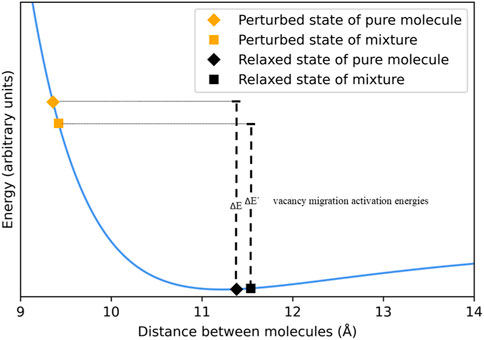
FIGURE 1. Lennard-Jones curve with four points highlighted, representing a snapshot of the effective distance between neighbors in both the relaxed and perturbed states of a mixture and a pure molecule.

The difference in the potential energy between the perturbed and relaxed configurations is symbolized as the difference in energy between the respective notional points corresponding to these states. As Jones (Jones, 1924) observed 100 years ago, the viscosity of a liquid scales exponentially with this energy difference and Eyring (Eyring, 1936) soon thereafter expressed this relationship in terms of transition state rate theory. Eq. 3 describes this relationship, where $\overline{\Delta E}$ is an integrated average of many terms like the one described above, $k$ is Boltzmann’s constant, $T$ is temperature and $C$ is a proportionality constant. By substituting Eq. 3 into Eq. 2, the Arrhenius blending rule for viscosity can be recast as Eq. 4.

$\mu =C*exp\left(\overline{\mathit{\Delta }E}/kT\right)(3)$

$\overline{\mathit{\Delta }{E}_{mix}}\approx {\displaystyle \sum }_i{x}_i*\overline{\mathit{\Delta }{E}_i}(4)$

As this discussion focuses on one representative set of structures the accent (representing average) is heretofore removed. The objective, re-stated, is to understand conceptually how mixing influences the accuracy of Eq. 4. It is worth noting however that the temperature dependence implied by Eq. 3 is significantly simpler than a variety of empirically derived relationships (Sloane and Winning, 1931; Link and de Klerk, 2022) that are more accurate over a limited temperature range, which implies that $\Delta E$ is also temperature dependent.

The total potential energy of the system at any instant in time ($\left.V\left(t\right)\right)$ is expressed by Eq. 5, where the summation runs over all molecules in the system. $V_{mn}$ is a 2-body interaction potential where the subscripts refer to the identity of the molecules rather than specific molecules, and $r_{ij}$ is the instantaneous distance between the pair of molecules, $i$ and $j$. To make this expression solvable, logic must be included to match the appropriate pairwise potential with the identity of the $i$th and $j$th molecules and to shed terms (beyond some threshold distance) that are negligible.

$V\left(t\right)={\displaystyle \sum }_i{\displaystyle \sum }_{j<i}{V}_{mn}\left(r_{ij}\right)(5)$

The model employed for this discussion affords significant simplification to Eq. 5. Two instants in time are considered. One corresponds to a spatial arrangement of molecules within the control volume that matches the relaxed state and the other instant corresponds to a spatial arrangement that matches the perturbed state. The only terms inside the sum that are different between these two instances, to first order, are those involving the migrating molecule.

In the relaxed state there are 11 such terms, each attractive with a contribution to the total energy that is approximately equal to the minimum in its 2-body potential energy curve ($\epsilon$). In the perturbed state, there are 18 such terms including six different values. In each case, where $r_{ij}$ of the perturbed state is higher than the lattice spacing, their sum is less exothermic than they are in relaxed state, $\epsilon$ or $2\epsilon$ depending on whether there are two or four such terms. While these terms are significant, it is the two pairs of points with $r_{ij}$ less than the lattice spacing that contribute the most to $\Delta E_i$. Our goal therefore is to understand how mixing may impact, especially these two pairs of terms.

Consider next the importance of the size of the sphere, before considering a mixed system. Assuming the same proportionality of vacancies and molecules as a smaller lattice and the same dative bond strength of the larger and smaller molecules, the system of larger molecules will have higher viscosity primarily because the encroachment distance ($r_{en}$) scales linearly with the lattice spacing ($D_L)$ and the repulsive forces between molecules increases sharply as $r_{en}$ increases.

$r_{en}=\left(1-\cos \left(30\right)\right)*D_L(6)$

Analogous to reaction rate theory, the molecular hops that accompany vacancy migrations will preferentially follow the path of least resistance. Along this path the smallest molecule in the control volume makes the hop. Intuitively, $\Delta E_{mix}$ should be lower than mole-fraction-weighted sum of $\Delta E_i$, contrary to Eq. 4. Indeed, a bias toward over-predicted values should be expected from the Arrhenius blending rule. The data, however, do not show this to be true. In the next few paragraphs, the impact of molecular-scale and cluster-scale mixing, respectively are considered on $\Delta E_{mix}$, $\overline{V_{mix}}$, the freeze point of a mixture and the enthalpy of mixing.

Figure 2 illustrates one possible arrangement of a 50/50%_mol mixture of a large and a small spherical molecule, mixed on a molecular scale. Both the relaxed and the perturbed states are shown, for effect, with no local distortion of the ccp lattice. None of the homogeneous, nearest neighbor interactions in the relaxed state are located close to the minimum of their respective 2-body potential energy curve. To second order, not shown, some distortion of a ccp lattice symmetry would occur, bringing some of the adjacent, smaller molecules closer together and some of the adjacent, larger molecules further apart. However, such a ripple effect would not be large relative to the salient point. If mixed on a molecular scale the potential energy of the relaxed state would be significantly higher than the mole-fraction-weighted sum of the components’ relaxed-state potential energies. The same cannot be said regarding the perturbed state. The salient point can be made by focusing on the four closest neighbors to the migrating molecule in the perturbed state. Even to first order, two of the corresponding terms in the potential energy sum (Eq. 5) are exothermic as the migrating, small molecule approaches a distance relative to two other small molecules (in this example) that is closer to the minimum of the relevant 2-body potential energy curve than any of the homogeneous terms of for the relaxed state. These two molecules are called out in Figure 2 by a solid gold border. Moreover, the encroachment distance relevant to the other two molecules in this quartet is not any larger than the corresponding distance in a purely homogeneous liquid. If mixed on a molecular scale, the potential energy of the perturbed state would be significantly lower than the mole-fraction-weighted sum of the components’ perturbed-state potential energies. Therefore, $\Delta E_{mix}$ would be significantly lower than the mole-fraction-weighted sum of $\Delta E_i$, and the viscosity of the mixture would be significantly lower than predicted by the Arrhenius blending rule, contrary to empirical evidence.

FIGURE 2

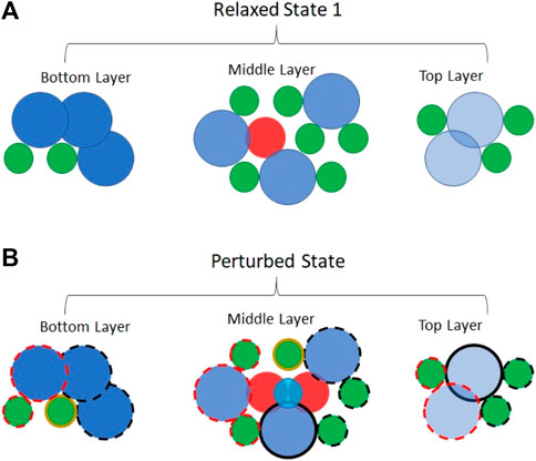
FIGURE 2. Molecular scale mixing of molecules within a ccp lattice of spacing equal to $D_n/1.5$. Three layers consisting of 5, 10, or 5 lattice vertices are shown (upper panel) One of the two interior vertices of the control volume is vacant (red circle) while the other is occupied by the smaller (green circle) of two molecules. Each of the remaining vertices is filled at random (50/50) with a smaller or larger (blue circle) molecule (lower panel) Much like the upper panel except the interior molecule is shifted by ½ the lattice spacing toward the vacancy. Endothermic changes (bottom view to top view) are denoted with black borders. Exothermic changes are denoted by red or gold borders. The solid borders represent the four interaction terms that are most important to viscosity. The dashed borders represent terms that are small in the perturbed state.

Returning now to the relaxed state, measured heats of mixing (Lundberg, 1964) do tend to be endothermic (∼0.03 kJ/mol) but significantly smaller than a typical dative bond strength (∼3 kJ/mol). This is interesting because, theoretically, forcing large and small molecules into the same control volume within a ccp packing arrangement causes several of the dative bonds to be significantly stretched or compressed. Breaking the symmetry of the model system and allowing its molar volume to exceed that of an ideal solution, the modeled endothermicity would move closer to measured values, but this would come at the expense of overpredicting the molar volume of the mixture. A convenient hypothesis to mitigate these conflicts is to mix on cluster scale rather than a molecular scale. Another model hypothesis that could match the observed viscosity, molar volume, and heat of solution is one that would decrease the concentration of vacancies in the mixed state relative to the unmixed components. However, this hypothesis does not explain freeze point observations. The freeze point of a mixture depends almost entirely on the thermal properties of the highest-freeze-point component and its mole fraction (Boehm et al., 2022), and a high degree of separation occurs as a result of the phase change.

The homogeneous clusters within liquid mixtures theoretically contain enough molecules such that the number of relevant (e.g., nearest neighbors) heterogeneous terms in Eq. 5 is small relative to the number of relevant homogeneous terms. Within each cluster the local molar volume and rate of vacancy migration (aka viscosity) is theoretically the same as it is in the respective pure component. The entropy of the model mixture varies according to random variation in cluster size. It also varies with the ratio between cluster and boundary volumes because the boundaries necessarily contain a considerable number of heterogeneous, intermolecular interactions. A symbolic representation of possible cluster size distributions is provided in Figure 3. As temperature increases, entropy becomes more important, driving smaller mean cluster size relative to the boundaries between clusters, a wider distribution of cluster sizes (relative to the mean) and a higher concentration of vacancies.

FIGURE 3

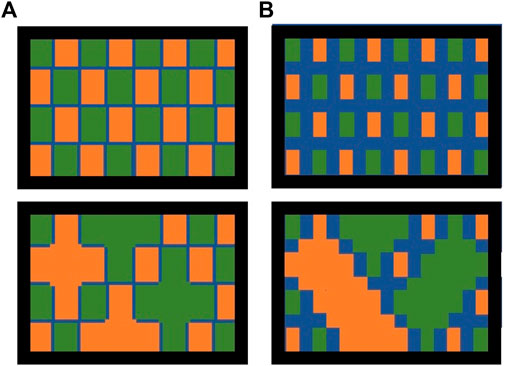
FIGURE 3. Possible arrangements of molecular clusters within the liquid phase. Orange represents one molecular species and green represents another molecular species. The blue lines represent boundaries between different clusters of molecules and are mixed at a molecular scale. (A) Large cluster sizes, enthalpy-controlled packing arrangement. (B) Small cluster sizes, entropy-controlled packing arrangement. In the top views, clusters of comparable size are distributed uniformly throughout the liquid phase. In the bottom views, clusters of variable size are distributed throughout the liquid.

The concentration of vacancies within the boundary regions is not known, which is especially important because the error in Eqs 1, 2 (ideal solution and Arrhenius blending rule) originate there. Theoretically, the rate of vacancy migration through the boundary region will preferentially follow the path of least resistance, which usually will involve the hop of a smaller molecule to an adjacent, vacant lattice site. The total potential energy of the relaxed state remains higher than the mole-fraction-weighted sum of the components’ potential energies even though structural distortions within the boundary regions lead to higher molar volume. Moreover, the total potential energy of the perturbed state remains lower than the mole-fraction-weighted sum of the components’ potential energies. In this respect, a correlation between higher-than-predicted molar volume and lower-than-predicted viscosity is expected (in a prevailing sense, not absolute), even within the cluster-mixing scheme. To get higher viscosity, a tighter-than-predicted packing arrangement is necessary. A convenient explanation for this would be a reduction in vacancies with mixing, which would tend to offset the entropy gained by chaotic placement of dissimilar molecules.

Of course, not all liquids have a molecular structure that is fundamentally close pack (ccp or hcp). For some molecules, it is exothermic relative to a close pack arrangement to bring some of the (12) nearest neighbors closer to the central atom. In these instances, the viscosity of the pure material would likely be lower than it would be if the ccp lattice packing arrangement were to be forced because the actual vacancy migration will preferentially follow the path of least resistance. This path would involve a perturbed state where distances between the traveling molecule and its four closest neighbors would be greater (closer to the minimum in the curve) than they would be in a ccp lattice. When such a material is mixed with some other material, the resulting lattice packing arrangement, particularly in the boundary region could be tighter than the pure material. This would explain lower-than-predicted molar volume, but the impact of such changes in the fundamental packing arrangement on the viscosity of the mixture is not clear. In this sense, the correlation between molar volume prediction error and viscosity prediction error should not be expected to fully explain the viscosity prediction error.

For mixtures involving components with a large difference in molar volume, it is possible for some or all the smaller molecules in the relaxed state to be positioned within the interstitial cavities of the packing arrangement of the larger molecules. The molar volume of such a mixture would be less than predicted by the ideal solution approximation. Its viscosity would be heavily influenced by heterogeneous interactions. The potential energy of the relaxed state could be exothermic relative to the separated liquids if the two-body heterogeneous potential energy curve has a deeper well than that of the two-body potential energy curve of the smaller component. In the perturbed state, the smaller, traveling molecule would have pushed into four larger molecules as it hopped from one interstitial site to another. Such a scenario is however unlikely for any binary pair of molecules within the jet fuel volatility range and extremely unlikely for complex mixtures such as jet fuel.

None of the neglects of potentially important structural difference between reality and the model system (mixture-driven change in fundamental packing arrangement, mixture-driven change in vacancy concentration, or local geometric distortion) are expected to create a linear correlation between viscosity and molar volume prediction errors. Nevertheless, we tried to improve/tailor the Arrhenius blending rule for our application by linearly regressing its error with molar volume differences amongst the components and molar volume prediction error. No improvement was found. Potential correlations between viscosity prediction error and the depth of the two-body potential energy curves were also explored by varying the fraction of aromatic hydrocarbons relative to saturated hydrocarbons. No such correlation was found.

The number of different molecules within the mixture may or may not impact the size distribution of homogeneous clusters, but the boundaries between clusters will be infused with a variety of distinct species. This provides for higher entropy with a potential impact on vacancy concentration. That issue aside, vacancy migrations through the boundary regions will preferentially follow the path of least resistance. This path involves migration of the smallest molecule from one lattice site to an adjacent lattice site that is vacant. Along the path of least resistance, the (usually 4) encroachment distances that matter most to the net endothermicity of the perturbed state can be driven to higher or lower values by infusing the lattice with other molecules that impact the lattice spacings. However, the main effect on the potential energy of the perturbed state is the fraction of these four terms that involve the largest molecule in the control volume. The potential energy of the relaxed state is also principally determined by the fraction of pairwise interactions that are compressed relative to the minimum of two-body potential energy curve.

The difference between (say) a four-component mixture and the mole-faction-weighted sum of two binary mixtures is not expected to be as large as the difference between a binary mixture and the mole-fraction-weighted sum of two pure components for several reasons. A complex mixture of simple mixtures is more likely to have the same fundamental packing arrangement as each of its component mixtures. The potential energy of the relaxed state of the complex mixture is expected to be much closer to the mole-fraction-weighted sum of its component, simple mixtures than it would be to the mole-fraction-weighted sum of its pure components. Likewise, the potential energy of the perturbed stated of a complex mixture is expected to be more like the perturbed state of simple mixtures than the perturbed state of pure components. The change in entropy resulting from a change in vacancy concentration within the boundary region is largest in systems that have the most order and smallest in the most chaotic systems. To evaluate these points in this work, mixtures of varying complexity were made and the inputs to Eqs 1, 2 were taken from direct measurement of the properties of each of two components whether those components were pure or themselves a mixtures of different molecules.

As evidenced by the increase of molar volume with temperature exhibited by most if not all liquids, vacancy concentration increases with temperature. The probability that a central molecule will be adjacent to a vacancy goes up proportionally so naturally the rate of vacancy migrations goes up and the corresponding viscosity goes down. The probability of a vacancy being one of the (usually four) closest neighbors to the central (traveling) molecule of the perturbed state also goes up. Therefore, temperature also impacts the endothermicity of the perturbed state and $\Delta E$. To second order the impact of higher vacancy concentration is manifested via an increased probability that a neighboring lattice site to any of the (usually) four nearest neighbors to the central molecule of the perturbed state will be vacant. A vacancy at any of those locations facilitates local geometric distortion of the perturbed state, thereby reducing its endothermicity and further reducing $\Delta E$.

For mixtures, the impact of increasing vacancy concentration on viscosity and molar volume is more complicated. For a control volume within a boundary region, the higher vacancy concentration affords more room for geometric distortions that drive down the potential energy of the relaxed state. Analogous to pure components, the potential energy of the perturbed state of the mixed system is also expected to decrease, but the magnitude of this decrease is hard to predict. Overall, the effect on increasing vacancy concentration, via increasing temperature, is expected to impact $\Delta E_{mix}$ differently than $\Delta E_i$. In this work temperature is varied to investigate these impacts.

3 Experimental

3.1 Controlled variables

Vacancy concentration: Measurements of each mixture and its blend components were taken at five different temperatures from −40°C to +15°C. The two lower temperatures, −40 and −20°C were motivated by industry requirements (D02 Committee, 2020) and the higher temperatures were selected to further investigate this derivative.

Strength of dative bond: Mixtures involving varying amounts of aromatic species were created for this investigation. The impact of this variation was monitored by tracking viscosity prediction error with the mixing-driven change in the fraction of heterogeneous terms that involve one aromatic hydrocarbon and one saturated hydrocarbon.

Lattice packing mismatch: Fifteen different molecules with molar volumes at −20°C ranging from 108.6 to 279.1 cm³/mol served as a base stock for 45 different binary mixtures and 36 different trinary mixtures. The impact of this variation was monitored by tracking viscosity prediction error with a plurality of simple algebraic combinations of the components molar volume and mole fraction. The lists of materials are provided in Tables 1, 2. The reported molar volumes at −20°C are from this work, while the reported phase transition temperatures are from one or more of the on-line data sources; PubChem, ChemSpider or NIST WebBook. The complete list of mixtures considered, including volume fraction of each component is provided in the supporting material along with measured density and viscosity data.

TABLE 1

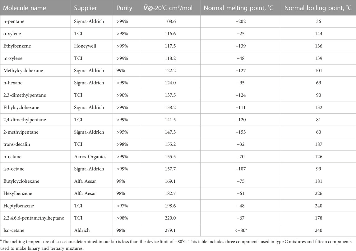
TABLE 1. List of pure materials used as stock for the mixtures investigated.

TABLE 2

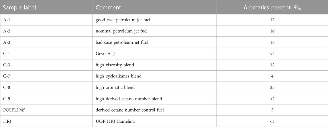
TABLE 2. List of complex mixtures (fuels) as stock for the mixtures investigated. The supplier of each of these fuels and data was the air force research laboratory, Fuels Branch (Edwards, 2017; Altjetfuels, 2021).

Mixture complexity: Four types of pseudo-binary mixtures were used to investigate the role of mixture complexity on viscosity prediction error. Each mixture (the left side of Eqs 1, 2 was comprised of two components (the right side of Eqs 1, 2, which themselves varied in complexity. A specific description of the four types of mixtures is provided in Table 3.

TABLE 3

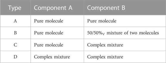
TABLE 3. Definition of mixture complexity types.

3.2 Materials and mixtures

Table 4 provides a listing each type A mixture pair. The molar volume mismatch between the respective pairs of pure molecules varies from 1.8 cm³/mol to 156.9 cm³/mol. Nine of the mixtures involve only saturated hydrocarbons, two involve only aromatic hydrocarbons, and eight involve one of each.

TABLE 4

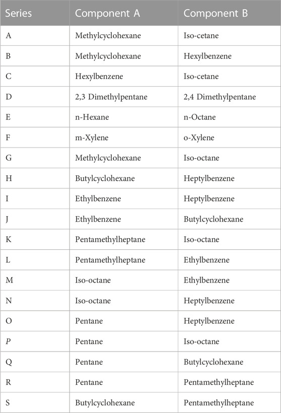
TABLE 4. Components of type A, binary mixtures.

Type B mixture pairs are listed in Table 5. The molar volume differences between the pure component and the average of the mixture component varies from 4.0 cm³/mol to 88.4 cm³/mol. Three of these mixtures involve saturated hydrocarbons exclusively, while a variety of aromatic/saturated blend fractions were sampled by the other mixtures.

TABLE 5

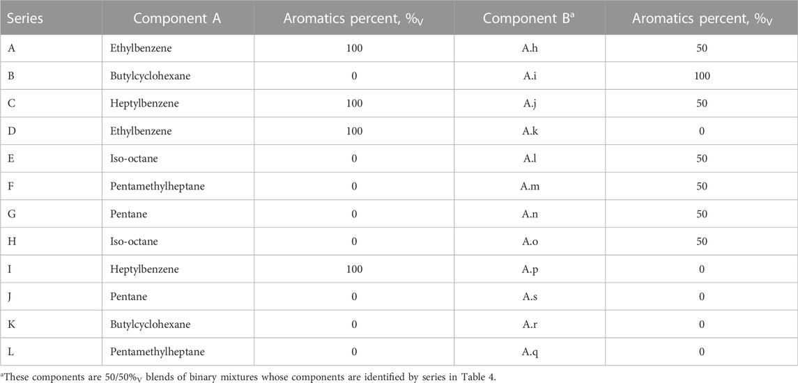
TABLE 5. Components of type B, tertiary mixtures.

Table 6 includes a listing of each type C and type D mixture. While the aromatic content varies significantly in these mixtures, this variety was used to reinforce or repudiate trends derived from the type B mixtures rather than elucidate any new trends. The type D mixtures represent a statistically significant range of the types of mixtures that may result from the blending of sustainable alternative fuel (SAF) components with other jet fuels. Molar volume difference between the two components of these blends varies between 0.1 cm³/mol (0% relative difference, %_RD) and 48.8 cm³/mol (23.5%_RD).

TABLE 6

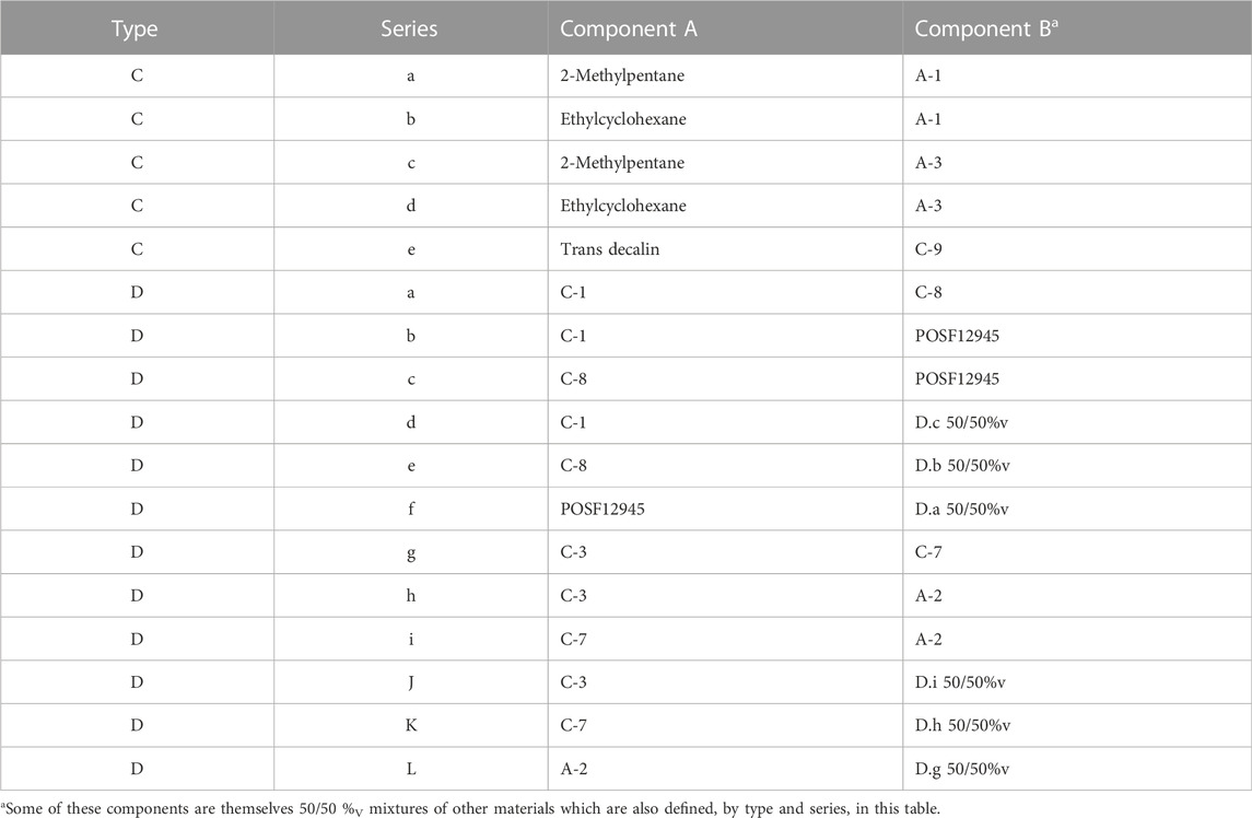
TABLE 6. Components of types C and D mixtures.

Six milliliters of each mixture were prepared using a set (0.5–5.0 ml) of volumetric pipettes, accurate to within 0.39%, to transfer the chemicals using standard laboratory procedures. Mixtures were swirled in a small beaker or vial for 1 minute prior to injecting 4 mL into the viscometer at room temperature. Viscosity and density measurements were taken at each temperature while chilling at a rate of 3.5 per minute, starting at 15°C and working down to −40°C.

3.3 Viscosity and density measurement details

The Anton Paar Kinematic Viscometer, SVM 3001 was used to measure both viscosity and density. This viscometer is a Stabinger viscometer which uses the Couette method to determine the torque necessary to overcome the viscous forces of the sample. That measured torque, M was used to calculate the shear stress (τ) as described in Eq. 7 where L and R_b are the length and radius of the bob, respectively. The shear rate ($\dot{\gamma }$) can be calculated using Eq. 8, where R_c is the radius of the container and ω is the angular velocity. The kinematic viscosity equals the shear stress divided by the shear rate and density ($\rho )$, as given by Eq. 9.

$\tau =M/\left(2*\pi *R_b^2*L\right)(7)$

$\dot{\gamma }=2*\omega *R_c^2/\left(R_c^2-R_b^2\right)(8)$

$\mu =\tau /\left(\rho *\dot{\gamma }\right)(9)$

The manufacturer-quoted, viscosity repeatability of this device is 0.1% over a range of 0.2–30,000 cSt. Its temperature range is −60°C to +135°C with a repeatability of 0.005°C and a reproducibility of 0.03°C from 15–100°C and 0.05°C for temperatures outside that range. Its density measurement repeatability is 0.00005 g/cm³ from 0.6 to 3.0 g/cm³. However, the repeatability and reproducibility for similar types of devices, reported in ASTM D7042 (D02.07 Subcommittee, 2021) is significantly different from this quote. There, it is suggested that for jet fuels at −40°C the viscosity repeatability and reproducibility are 0.53% and 2.1% respectively, and the density repeatability and reproducibility are 0.197% and 0.203% respectively. Our own assessment of repeatability, using a small sub-set of the mixtures studied here and including mixture preparation repetition was found to be 0.26% and 3.2% for density and viscosity, respectively. Most of this variation is believed to be the result of mixture preparation variation, particularly mixtures involving solvents with very low surface tension and high vapor pressure at room temperature.

For this study, viscosity and density were collected at fluid temperatures of 15, 0, −10, −20, and −40°C. At each temperature increment, viscosity and density measurements were recorded over a narrower range of temperatures. For example, at 15°C, the viscosity and density were measured over a temperature range of 14.999°C–15.001°C.

From start to finish, the test campaign extended over a period of several months, but data collections pertaining to any given series was completed within weeks. All data pertaining to type D mixtures and about 2/3^rds of the data pertaining to type A mixtures were collected under one calibration of the device while the remainder was collected under another calibration. None of the series identified in section 3.2 included mixed-calibration data. The SVM 3001 viscometer calibration is performed annually with a manufacturer technician on site. For temperature calibration, Anton Paar MKT 10 is used to establish the reference data vector. For viscosity and density calibration, a manufacturer-certified, standard oil is used to establish the reference data. In-between the annual calibrations of the device, the drift in viscosity and density measurement is determined by our lab to be less than 1%.

While measurement uncertainty was low, it is further noted here that systematic measurement error that is correctable by a constant scale factor would have no bearing on the blending rule error quantification. Moreover, systematic error that is correctable by a constant off-set value would affect the apparent modeling error by approximately 1% of the off-set value. However, unidentified systematic error that varies with torque or angular velocity could potentially impact the blending rule error quantification significantly. The current viscosity measurements at low temperature (−40°C–15°C) were therefore compared with twelve other recent measurements, as provided in the supporting material. Seven of our measured values are lower than those reported in the literature and five are higher. The standard deviation of the relative error across the fundamentally different measurement approaches was 8.8%. Such variation provides motivation to use, exclusively, data from the same laboratory to evaluate the accuracy of any blending rule for viscosity.

4 Results

All viscosity and density measurements were taken at ambient pressure and are provided within the supporting information of this manuscript. The prediction error, defined by Eq. 10, was regressed against several independent variables based on the concepts introduced in the theory section of this manuscript. A set of multilinear regressions were executed 30 times; once for each temperature and mixture type (20 sets), once with each mixture type with all temperature data pooled (4 sets), once for each temperature with all mixture types pooled (5 sets) and once with all data pooled together (1 set).

$Err\equiv \left({\mu }_{pred}/{\mu }_{meas}-1\right)\approx \ln {\mu }_{pred}-\ln {\mu }_{meas}\approx \left(∆E_{meas}-∆E_{pred}\right)/RT(10)$

A unity plot of the predictions relative to the measurements is shown in Figure 4. This plot shows that the prediction error does not correlate with viscosity magnitude and the Arrhenius blending rule captures 99.7% (R²) of the variation in the measured data, on a log scale. The regressed line through all data, pooled together has a slope of 0.990 with zero intercept. Another characteristic, evident in this plot is that data scatter decreases as mixture complexity increases, which is discussed further in the remainder of this section.

FIGURE 4

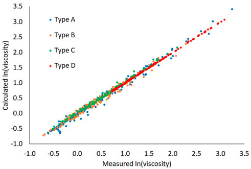
FIGURE 4. Unity plot. The reference viscosity is 1 cSt.

While several of these data subsets exhibited qualitatively similar correlations between prediction error and a variety of independent variables, few correlations persisted in all subgroups with similar magnitude and sign. For example, the molar volume difference between the mixture and its components, as two independent variables, are correlated with viscosity prediction error within all subgroups, having a probability of no correlation (p-value) less than 0.01. However, the magnitude and even the sign of the correlation coefficient changes from subgroup to subgroup. When all data are pooled together, only 1 molar volume difference term remains statistically significant. That one variable can be any of several algebraic combinations of the three relevant molar volumes and the two relevant mole fractions. The viscosity prediction error was also found to correlate with molar volume prediction error in most of the considered datasets and their respective correlation coefficients are also inconsistent across datasets. The molar volume prediction error is defined as the ratio of the predicted and measured values minutes one. The measured molar volume is the calculated molecular weight divided by the measured density and the predicted molar volume is the result of the ideal solution approximation, taking the measured components’ molar volume as input. The difference in aromatics concentration between the components was not found to correlate with viscosity prediction error.

The mixture complexity, its temperature and the molar volume prediction error are the most important indicators of viscosity prediction error. The temperature influence is not large, but its sign and approximate magnitude are consistent across all types of mixtures studied regardless of other independent variables considered, as summarized in Figure 5. The mean viscosity prediction error decreases non-linearly from a high of 1.68% at −40°C to a low of −0.13% at 15°C when data from all four types of mixtures are pooled. Its standard deviation also decreases as temperature increases. The decreasing mean error with increasing temperature suggests that the mixing has less effect on $\Delta E_{mix}$ as the concentration of vacancies increases.

FIGURE 5

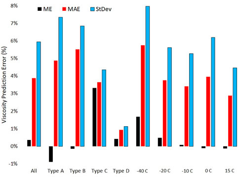
FIGURE 5. Measures of viscosity prediction error across differing mixture complexity and temperature. Mean error (ME), mean absolute error (MAE), standard deviation (StDev).

The mean prediction error increases with mixture complexity while the variation in that error decreases substantially. This is partially consistent with the theory which asserts that the potential energy of terms like $V_{bb}\left(r_{\mathit{min}}\right)$ in ABC mixtures will be closer to the value it has in BC mixtures, compared to the value it has in pure liquid, B. The theory suggests that both the mean error and its standard deviation should decrease with increasing mixture complexity. The opposite (as observed) impact on mean prediction error suggests that a greater variety of heterogeneous interactions imparts a bias toward closer two-body interactions in the perturbed state as necessary to accommodate certain vacancy migrations.

Figure 6 shows a plot of viscosity prediction error against molar volume prediction error. The prevailing inverse relationship between molar volume and viscosity prediction error is consistent with theory and is shaped primarily by the simpler mixtures, types A and B. If the predicted molar volume is higher than the actual molar volume then the predicted average distance between molecules in the relaxed state of the mixture is higher than it really is. In most cases, this would transfer to the perturbed state as well. Since the potential energy surface is highly non-linear, the artificially high spacing between molecules in the perturbed state leads to artificially low activation energy and correspondingly low viscosity predictions. While there is clearly a codependence between molar volume prediction error and other independent variables considered in this work, its inclusion as independent variable in multilinear regressions improves the R² significantly in most data subgroupings and never hurts the adjusted R². Conversely, it alone as a linear term, explains less than 20% of the variation in the complete dataset and less than 50% of the variation within any of the sub-groups considered. Moreover, the nominal slope of this relationship varies across the four sub-groups. The difference in molar volume between the components of a mixture is important but not sufficiently so to overshadow other important (and non-linear) effects.

FIGURE 6

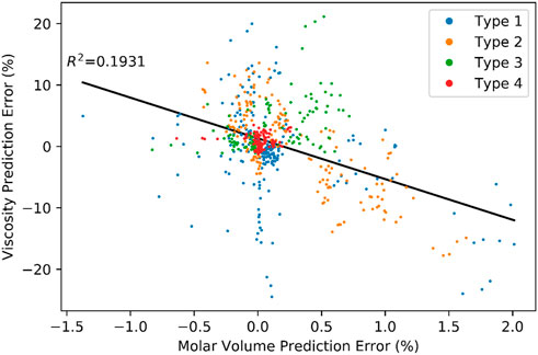
FIGURE 6. Viscosity and molar volume prediction error correlation.

These results do not suggest an improved blending rule for viscosity, relative to the Arrhenius blending rule, but they do suggest a way to quantify the error. The tier alpha (Yang et al., 2021) methodology for viscosity employs the Arrhenius blending rule, generalized to many components, where each component is a pure molecule. As such it employs pure molecule data exclusively. No heterogeneous interaction terms are implicitly included in the tier alpha model, meaning the errors introduced by Eq. 4 are not partially captured by data inputs as they are in this work for types B, C and D mixtures. The error introduced by the tier alpha approach therefore is analogous to those of the type A mixtures of this work. The observed error ($\sigma$) in the predictions for type A mixtures can be attributed to each term ($\xi$) equally by presumption, as represented by Eq. 11. The observations reported here suggest $\xi$

${\sigma }^2={\left(x_A*\xi \right)}^2+{\left(x_B*\xi \right)}^2={\xi }^2*{\displaystyle \sum }_i{x}_i^2(11)$

equals 13.2% at −40°C and 9.6% at −20°C. To impart such modelling error onto the tier alpha predictions, the term relating to measured viscosity uncertainty should be replaced by the composite of measurement uncertainty and the result of Eq. 11. Because every component mole fraction in complex mixtures is small, in most cases, this error term will also be small. Non-etheless, it is expected to resolve the small miss at low temperatures noted by Heyne et al. (Heyne et al., 2022) for a fuel with determined identity of specific isomers accounting for 94%_m of the composition

5 Conclusion

Six hundred and seventy-five measurements of dynamic viscosity and density have been used to assess the prediction error of the Arrhenius blending rule for kinematic viscosity of hydrocarbon mixtures. Major trends within the data show that mixture complexity and temperature are more important determinants of prediction error than differences in molecular size or hydrogen saturation between the components of the mixtures. Over the range evaluated, no correlation to mole fractions was observed, suggesting the log of viscosity truly is linear in mole fraction, as indicated by the Arrhenius blending rule. Mixture complexity and temperature also impact molar volume and its prediction. However, a linear regression between the two model errors explains less than 20% of the observed variation, indicating that mixture viscosity and/or molar volume are not linear with respect to temperature and/or mixture complexity.

Because the main effects, namely mole fractions are already captured by the Arrhenius blending rule for viscosity while other, lesser influence factors such as changes to vacancy distribution, the distances between nearest neighbors and the number percentage and variety of heterogeneous interactions, each have a complex impact on viscosity it is difficult to refine the model. Moreover, each of these fundamental drivers are hard to control independently in an experiment, rendering an empirically driven correction to the Arrhenius blending rule elusive as well. Nonetheless, sufficient data has been collected to measure the prediction error. That information has been transferred back to the model to enable direct determinations of confidence intervals around subsequent viscosity predictions of any fuel based on its component mole fractions and viscosities. At −40°C, when all identified components are pure molecules the modeling error is 0.132 times the predicted (nominal) viscosity times the root mean square of the component mole fractions. At -20 °C the scalar decreases to 0.096 as part of a general trend observed here that viscosity prediction errors decrease as temperature increases.

6 Supporting information

All the viscosity and density data measured in support of this manuscript are provided within the “data” tab of the attached document called HEAT_LAB_ViscosityData_2022 (XLSX). Expanded versions of Tables 1, 2 are provided in the other tab, “Material_list”. A definition of important terms used throughout the theory section is provided in Viscosity_molecular_level (DOCX).

Data availability statement

The original contributions presented in the study are included in the article/Supplementary Material, further inquiries can be directed to the corresponding author.

Author contributions

RB Writing, theory, data analysis FH Data acquisition, editing, data analysis support ZY Data acquisition guidance, editing, literature data, figures TW Literature review, writing, editing JH Project funding and conceptualization.

Funding

Support for this work (data collection, data analysis, and first manuscript draft) was provided by U.S. DOE BETO through subcontract PO 2196073. Additional support (manuscript revision and publication fees) was provided by the U.S. Federal Aviation Administration Office of Environment and Energy through ASCENT, the FAA Center of Excellence for Alternative Jet Fuels and the Environment, project 065a through FAA Award Number 13-C-AJFE-UD-026 under the supervision of Dr. Prem Lobo. Any opinions, findings, conclusions, or recommendations expressed in this material are those of the authors and do not necessarily reflect the views of the FAA.

Conflict of interest

The authors declare that the research was conducted in the absence of any commercial or financial relationships that could be construed as a potential conflict of interest.

Publisher’s note

All claims expressed in this article are solely those of the authors and do not necessarily represent those of their affiliated organizations, or those of the publisher, the editors and the reviewers. Any product that may be evaluated in this article, or claim that may be made by its manufacturer, is not guaranteed or endorsed by the publisher.

Supplementary material

The Supplementary Material for this article can be found online at: https://www.frontiersin.org/articles/10.3389/fenrg.2022.1074699/full#supplementary-material

References

Alonso Saldana, D., Starck, L., Mougin, P., Rousseau, B., Ferrando, N., and Creton, B. (2012). Prediction of density and viscosity of biofuel compounds using machine learning methods. Energy fuels. 26, 2416–2426. doi:10.1021/ef3001339

CrossRef Full Text | Google Scholar

Altjetfuels, T. L. (2021). Home | AJF:TD | U of I n.d. https://altjetfuels.illinois.edu/.

Google Scholar

Arrhenius, S. A. (1887). On the internal friction of dilute aqueous solutions. Z Phys. Chem. 1, 285.

Google Scholar

Barabás, I., and Todoruţ, I-A. (2011). Predicting the temperature dependent viscosity of biodiesel–diesel–bioethanol blends. Energy fuels. 25, 5767–5774. doi:10.1021/ef2007936

CrossRef Full Text | Google Scholar

Bhethanabotla, V. R. (1983). A group contribution method for liquid viscosity. State College, PA: The Pennsylvania State University.

Google Scholar

Boehm, R. C., Coburn, A. A., Yang, Z., Wanstall, C. T., and Heyne, J. S. (2022). Blend prediction model for the freeze point of jet fuel range hydrocarbons. Energy fuels. 36, 12046–12053. doi:10.1021/acs.energyfuels.2c02063

CrossRef Full Text | Google Scholar

Boehm, R. C., Colborn, J. G., and Heyne, J. S. (2021). Comparing alternative jet fuel dependencies between combustors of different size and mixing approaches. Front. Energy Res. 9. doi:10.3389/fenrg.2021.701901

CrossRef Full Text | Google Scholar

Boehm, R. C., Scholla, L. C., and Heyne, J. S. (2021). Sustainable alternative fuel effects on energy consumption of jet engines. Fuel 304, 121378. doi:10.1016/J.FUEL.2021.121378

CrossRef Full Text | Google Scholar

Carlson, D. J., Giles, N. F., Wilding, W. V., and Knotts, T. A. (2022). Liquid viscosity oriented parameterization of the Mie potential for reliable predictions of normal alkanes and alkylbenzenes. Fluid Phase Equilib. 561, 113522. doi:10.1016/J.FLUID.2022.113522

CrossRef Full Text | Google Scholar

Centeno, G., Sánchez-Reyna, G., Ancheyta, J., Muñoz, J. A. D., and Cardona, N. (2011). Testing various mixing rules for calculation of viscosity of petroleum blends. Fuel 90, 3561–3570. doi:10.1016/J.FUEL.2011.02.028

CrossRef Full Text | Google Scholar

Colket, M., and Heyne, J. (2021). Fuel effects on operability of aircraft gas turbine combustors. August. AIAA. Prog. Astronautics Aeronautics. doi:10.2514/4.106040

CrossRef Full Text | Google Scholar

Cramer, J. A., Hammond, M. H., Myers, K. M., Loegel, T. N., and Morris, R. E. (2014). Novel data abstraction strategy utilizing gas chromatography–mass spectrometry data for fuel property modeling. Energy fuels. 28, 1781–1791. doi:10.1021/ef4021872

CrossRef Full Text | Google Scholar

D02 Committee, (2020). Astm D7566: Specification for aviation turbine fuel containing synthesized hydrocarbons. Conshokocken, PA, USA: ASTM International. doi:10.1520/D7566-20

CrossRef Full Text | Google Scholar

D02.07 Subcommittee (2021). ASTM D7042 standard test method for dynamic viscosity and density of liquids by stabinger viscometer (and the calculation of kinematic viscosity), https://wiki.anton-paar.com/in-en/basic-of-viscometry/astm-d7042/. doi:10.1520/D7042-21A

CrossRef Full Text | Google Scholar

Edwards, T. (2017). “Reference jet fuels for combustion testing,” in AIAA SciTech Forum - 55th AIAA Aerosp. Sci. Meet (Grapevine, TX, USA: American Institute of Aeronautics and Astronautics Inc.), 1–58. doi:10.2514/6.2017-0146

CrossRef Full Text | Google Scholar

Eyring, H. (1936). Viscosity, plasticity, and diffusion as examples of absolute reaction rates. J. Chem. Phys. 4, 283–291. doi:10.1063/1.1749836

CrossRef Full Text | Google Scholar

Fraser, R. P. (1957). Liquid fuel atomization. Symposium Combust. 6, 687–701. doi:10.1016/S0082-0784(57)80096-4

CrossRef Full Text | Google Scholar

Galliéro, G., Boned, C., and Baylaucq, A. (2005). Molecular dynamics study of the Lennard−Jones fluid viscosity: Application to real fluids. Ind. Eng. Chem. Res. 44, 6963–6972. doi:10.1021/IE050154T

CrossRef Full Text | Google Scholar

Gaudin, T., and Ma, H. (2020). The macroscopic viscosity approximation: A first-principle relationship between molecular diffusion and viscosity. AIP Adv. 10, 035321. doi:10.1063/1.5131234

CrossRef Full Text | Google Scholar

Guildenbecher, D. R., López-Rivera, C., and Sojka, P. E. (2009). Secondary atomization. Exp. Fluids 46, 371–402. doi:10.1007/s00348-008-0593-2

CrossRef Full Text | Google Scholar

Hall, C., Rauch, B., Bauder, U., Le Clercq, P., and Aigner, M. (2021). Predictive capability assessment of probabilistic machine learning models for density prediction of conventional and synthetic jet fuels. Energy Fuels 35, 2520–2530.

CrossRef Full Text

Hauck, F., Kosir, S., Yang, Z., Heyne, J., Landera, A., and George, A. (2020). Experimental validation of viscosity blending rules and extrapolation for sustainable aviation fuel. AIAA Propuls. Energy, 1–15. doi:10.2514/6.2020-3671

CrossRef Full Text | Google Scholar

Hernández, E. A., Sánchez-Reyna, G., and Ancheyta, J. (2021). Evaluation of mixing rules to predict viscosity of petrodiesel and biodiesel blends. Fuel 283, 118941. doi:10.1016/J.FUEL.2020.118941

CrossRef Full Text | Google Scholar

Heyne, J., Bell, D., Feldhausen, J., Yang, Z., and Boehm, R. (2022). Towards fuel composition and properties from Two-dimensional gas chromatography with flame ionization and vacuum ultraviolet spectroscopy. Fuel 312, 122709. doi:10.1016/J.FUEL.2021.122709

CrossRef Full Text | Google Scholar

Hosseini, S. M., Pierantozzi, M., and Moghadasi, J. (2019). Viscosities of some fatty acid esters and biodiesel fuels from a rough hard-sphere-chain model and artificial neural network. Fuel 235, 1083–1091. doi:10.1016/J.FUEL.2018.08.088

CrossRef Full Text | Google Scholar

Hsu, H. C., Sheu, Y. W., and Tu, C. H. (2002). Viscosity estimation at low temperatures (Tr<0.75) for organic liquids from group contributions. Chem. Eng. J. 88, 27–35. doi:10.1016/S1385-8947(01)00249-2

CrossRef Full Text | Google Scholar

Johnson, K. J., Morris, R. E., and Rose-Pehrsson, S. L. (2006). Evaluating the predictive powers of spectroscopy and chromatography for fuel quality assessment. Energy fuels. 20, 727–733. doi:10.1021/ef050347t

CrossRef Full Text | Google Scholar

Jones, J. E. (1924). On the determination of molecular fields.—I. From the variation of the viscosity of a gas with temperature. Proc. R. Soc. Lond. Ser. A, Contain Pap. a Math. Phys. Character 106, 441–462. doi:10.1098/RSPA.1924.0081

CrossRef Full Text | Google Scholar

Kanaveli, I. P., Atzemi, M., and Lois, E. (2017). Predicting the viscosity of diesel/biodiesel blends. Fuel 199, 248–263. doi:10.1016/J.FUEL.2017.02.077

CrossRef Full Text | Google Scholar

Kumar, M., Karmakar, S., Kumar, S., and Basu, S. (2021). Experimental investigation on spray characteristics of Jet A-1 and alternative aviation fuels. Int. J. Spray Combust. Dyn. 13, 54–71. doi:10.1177/17568277211010140

CrossRef Full Text | Google Scholar

Lee, M. J., and Wei, M. C. (1993). Corresponding-states model for viscosity of liquids and liquid mixtures. J. Chem. Eng. Jpn. 26, 159–165. doi:10.1252/JCEJ.26.159

CrossRef Full Text | Google Scholar

Link, F., and de Klerk, A. (2022). Viscosity and density of narrow distillation cuts from refined petroleum and synthetic-derived distillates in -60 to +60 °C range. Energy fuels. 36. doi:10.1021/acs.energyfuels.2c02625

PubMed Abstract | CrossRef Full Text | Google Scholar

Lundberg, G. W. (1964). Thermodynamics of solutions XI. Heats of mixing of hydrocarbons. J. Chem. Eng. Data 9, 193–198. doi:10.1021/je60021a013

CrossRef Full Text | Google Scholar

Maginn, E. J., Messerly, R. A., Carlson, D. J., Roe, D. R., and Elliot, J. R. (2019). Best practices for computing transport properties 1. Self-diffusivity and viscosity from equilibrium molecular dynamics [article v1.0]. Living J. comput. Mol. Sci. 1, 6324. doi:10.33011/livecoms.1.1.6324

CrossRef Full Text | Google Scholar

Mondello, M., and Grest, G. S. (1998). Viscosity calculations ofn-alkanes by equilibrium molecular dynamics. J. Chem. Phys. 106, 9327–9336. doi:10.1063/1.474002

CrossRef Full Text | Google Scholar

Przedziecki, J. W., and Sridhar, T. (1985). Prediction of liquid viscosities. AIChE J. 31, 333–335. doi:10.1002/AIC.690310225

CrossRef Full Text | Google Scholar

Reid, R. C., Prausnitz, J. M., and Poling, B. E. (1987). The properties of gases and liquids. Web Osti.Gov: U.S. Department of Energy, Office of Scientific and Technical Information.

Google Scholar

Sloane, R. G., and Winning, C. (1931). Viscosity-temperature relationship of lubricating oils. Ind. Eng. Chem. 23, 673–674. doi:10.1021/ie50258a017

CrossRef Full Text | Google Scholar

Teja, A. S., and Rice, P. (1981). Generalized corresponding states method for the viscosities of liquid mixtures. Ind. Eng. Chem. Fundam. 20, 77–81. doi:10.1021/I100001A015/ASSET/I100001A015

CrossRef Full Text | Google Scholar

Thomas, L. H. (1942). The dependence of the viscosities of liquids on reduced temperature, and a relation between viscosity, density, and chemical constitution. J. Chem. Soc., 573–579. doi:10.1039/jr9460000573

PubMed Abstract | CrossRef Full Text | Google Scholar

van Velzen, D., Cardozo, R. L., and Langenkamp, H. (1972). A liquid viscosity-temperature-chemical constitution relation for organic compounds, Ind. Eng. Chem. Fundam., 11. PNG_V03: FP, 20–25. doi:10.1021/I160041A004/ASSET/I160041A004

CrossRef Full Text | Google Scholar

Vozka, P., and Kilaz, G. (2020). A review of aviation turbine fuel chemical composition-property relations. Fuel 268, 117391. doi:10.1016/j.fuel.2020.117391

CrossRef Full Text | Google Scholar

Yang, Z., Kosir, S., Stachler, R., Shafer, L., Anderson, C., and Heyne, J. S. (2021). A GC × GC Tier α combustor operability prescreening method for sustainable aviation fuel candidates. Fuel 292, 120345. doi:10.1016/j.fuel.2021.120345

CrossRef Full Text | Google Scholar

Nomenclature

Acronyms

ASTM ASTM international, standards organization

cSt centistoke unit of kinematic viscosity

ME mean error

MAE mean absolute error

SAF sustainable aviation fuel or fuels

StDev standard deviation

Symbols and Labels

A,B,C,D mixture types delineating the number of distinct species present from 2 A) to many D)

E total potential energy

L length of bob used in experimental apparatus

M measured torque

N number of molecules

R universal gas constant

R² coefficient of determination

Rb, Rc radius of bob and sample chamber respectively used in experimental apparatus

r distance between molecules

D_L lattice spacing

T temperature

V potential energy terms

$\overline{V}$ molar volume

x mole fraction

Δ difference between two sets of defining conditions

$\dot{\gamma }$ shear rate

$\tau$ shear stress

$\omega$ angular velocity

$\rho$ density

$\mu$ kinematic viscosity

$\sigma$ observed error or uncertainty

$\xi$ uncertainty attributed to each pure component

Subscripts

i, j molecule tracking indices, regardless of molecular identity

m,n,a,b identifiers of molecular identity

A,B msixture component tracking indices, regardless of component complexity

mix mixture

aro aromatic

meas measured

pred predicted