Curve and double-layer economic dispatching considering reasonable wind abandonment under different time granularities

In view of the large output of wind power during the load trough time, the peak regulation cost may increase sharply, and the traditional hourly dispatch may not be able to accurately track the load fluctuation due to the fluctuation of renewable energy. In this paper, based on different time granularities, an adaptive segmented double-layer economic scheduling model of the net load curve considering reasonable wind abandonment is constructed. The model can better cope with net load changes while reducing the load peak-to-valley difference. First, a reasonable wind abandonment model is established under different time granularities of 5 min, 15 min, 30 min, and 1 h; Then, based on the static thinking of the net load curve by time period, the load change in the hourly scale is fully considered without changing the total number of dispatching periods so that each dispatching period can adaptively select the duration according to the change of net load gradient, and a self-adaptive subsection model of the net load curve is established to minimize the total running cost. Finally, taking IEEE-30 nodes as the example system, the NSGA-II algorithm and CPLEX solver are used to solve the model. The results verify the economy and feasibility of the proposed model.

1 Introduction

As wind power, photovoltaic, and other new energy sources are greatly affected by the natural environment and have obvious randomness and volatility (Liu Y et al., 2021; Hao C A et al., 2021; Guo T et al., 2020), full consumption of wind power may cause a peak-to-valley difference, deep peak regulation, and sharp increase in peak regulation cost (Ming D A et al., 2021; Liu et al., 2022; Wei H et al., 2022; Wang J et al., 2021; Chen et al., 2021) and even cause a potential operation risk of the power grid (Zhou Y et al., 2021; Dall’Anese et al., 2018; Cheng et al., 2019; Deng et al., 2019; Luo et al., 2019). Therefore, when the wind power output is large and the load is low, selectively discarding part of the wind power output can not only reduce the operation risk of the power grid but also help to improve the flexibility of power grid dispatching and the overall economic benefits.

At present, based on the reality that appropriate wind abandonment can improve the economic benefits of the system, there are many studies that consider abandonment of wind power (Yang et al., 2020; Chen et al., 2020; Gan et al., 2022; Wang et al., 2022). Wanla et al. (2021) constructed the steady-state power flow of the integrated energy system through the coupling of power grid and heat network and constructs the collaborative optimization operation model of “source-grid-load-storage” of the integrated energy system with the goal of system economic operation to solve the curtailment air volume. Sun.et al. (2020) proposed an optimization method for the wind farm access capacity and access location considering the minimum wind curtailment and combines the minimum wind curtailment index and the highest reliability level index to optimize the wind power access capacity. Zang.et al. (2022) established the optimal energy abandonment constraint model, considering the characteristics of wind and solar reverse peak regulation, to improve the economy of wind and solar absorption of the system and the low carbon of thermal power peak shaving , and the net load curve is “peak shaving and valley filling.” The aforementioned literature proposes to realize the optimal operation of the system by abandoning part of the wind power and solves the problem of curtailed wind power, but fails to consider the change of curtailment volume over a timescale.

For dealing with the uncertainty of wind power, traditional hourly dispatch cannot flexibly deal with the fluctuations in the net load data. For this reason, most literatures coordinate day-ahead, intraday, and real-time dispatching (Dou.et al., 2019; Liu.et al., 2022), and coordination of multiple timescales is used to gradually reduce the impact of errors in an operation (Shi et al., 2019; Yang et al., 2021; Tang et al., 2022). Although this method can effectively reduce the deviation, the model usually participates in the day-ahead scheduling operation with an hour-level time resolution, ignoring the error caused by the approximate distribution of discrete time (Song.et al., 2021; Mz et al., 2021; Song.et al., 2021). The discrete time at the hour level cannot reflect the details of the gradient change of the net load, and the wind power may change greatly within the hour. Therefore, the traditional hour-level model cannot meet the demand for flexibility, and it is necessary to optimize the time interval more flexibly to better response to the changes in the net load.

Ran et al. (2020), according to the slow dynamic characteristics of cold and thermal energy, adopted the daily mixed timescale correction method of electric cooling thermal coupling, optimizes the output of cold and thermal energy-related equipment at the upper layer with a low time resolution, and adjusts the power storage device and tie line scheduling plan at the lower layer with a fine temporal resolution and the correction results of the upper layer, to build a mixed timescale economic scheduling model considering the difference of energy characteristics. Although this method improves the flexibility of the system, it also increases the computational complexity. Gan.et al. (2020), to solve quickly, proposed a renewable energy generation and demand load forecasting model with a coarse-grained resolution of 15 min or 1 hour using a single temporal resolution. It can be seen that while using fine temporal resolution saves operating costs, increasing the time interval leads to an exponential increase in the solution time. The model using hourly summarization, while reducing the computational complexity, does not accurately track changes in the net load.

In view of the aforementioned problems, first, reasonable wind curtailment models are established at different time granularities (Li.et al., 2022; Liu.et al., 2019), and its impact on the fluctuation of the net load curve and peak regulation cost is analyzed. Second, to accurately track the net load change, a segmentation model of the net load curve with an adaptive selection of scheduling duration is established. Finally, the impact of reasonable wind curtailment and adaptive segmentation of the load curve on power grid peak regulation and overall economy is comprehensively analyzed.

2 Reasonable wind abandonment models under different time granularities

Due to the anti-peak regulation characteristics of wind power, a few peak wind power output occurs in the low load period, to absorb more peak wind power output should reduce the system’s thermal power output, but at the same time lead to an increase in the cost of rotating backup, this will result in a sharp increase in the total operating costs of the system. In this regard, under different time granularities of 5 min, 15 min, 30 min, and 1 h, the optimization goal is to minimize the net load variance of the system, consider the constraints of wind power output and wind curtailment, establish an optimization model, and use the Cplex solver to solve it.

2.1 Objective function

Due to the uncertainty of load and wind power output, the peak-to-valley difference of the system power load is large, and the model ensures that the net load variance gradually decreases at the expense of discarding an appropriate amount of wind power generation, so that the net load curve is smoother (Zang.et al., 2022). The objective function is the minimum variance of the net load of the system, and its expression is given as follows:

${\mathrm{m}\mathrm{i}\mathrm{n}\mathrm{F}}_1=\frac{1}{T}{\displaystyle \sum }_{t=1}^T{\left(P{L}_{\mathrm{t}}-P{L}_{ave,t}\right)}^2,(1)$

$P{L}_{\mathrm{t}}=P_{d,t}-\left(1-{\lambda }_{w,t}\right)P_{w,t},(2)$

$P{L}_{ave,t}=\left({\displaystyle \sum }_{t=1}^{T}P{L}_t\right)/T,(3)$

where ${\mathrm{F}}_1$ is the system net load variance;t, respectively for 5 min, 15 min, 30 min and 1 h time series under different time granularity first t a period of time; ${PL}_t$ is the net load of the system in the t-th period; ${PL}_{ave,t}$ is the average value of the net load of the system in the whole scheduling period; ${\mathrm{P}}_{\mathrm{d},\mathrm{t}}$ is the initial load in the t-th period; ${\lambda }_{\mathrm{w},\mathrm{t}}$ is the wind abandon rate of the t-th period, $0\le {\lambda }_{\mathrm{w},\mathrm{t}}\le$ 1; and ${\mathrm{P}}_{\mathrm{w},\mathrm{t}}$ is the output power of the wind farm in the t-th period.

2.2 Constraint condition

The solution of the reasonable wind abandonment optimization model should satisfy the following constraints:

1) Wind power output constraints:

$0\le P_{w,t}\le P_{w,\mathit{max}},(4)$

where ${\mathrm{P}}_{\mathrm{w},\max }$ is the maximum output of the wind farm in the t-th period.

2) Abandon wind rate constraint:

To avoid a large amount of abandonment of wind farms due to the smoothing of the net load curve, the maximum allowable abandonment rate constraint is added to this paper, namely,

${\displaystyle \sum }_{t=1}^T{\lambda }_{w,t}{P}_{w,t}/{\displaystyle \sum }_{t=1}^T{P}_{w,t}\le k_{w,\max },(5)$

where ${\mathrm{k}}_{\mathrm{w},\max }$ is the maximum wind abandonment rate allowed by the wind field.

3 Net load curve self-adaptation segment optimization model

Based on the abovementioned model, under the different time granularities, based on the idea of load curve segmenting into time-segment statics, the continuous typical daily load curve can be reasonably segmented, which will effectively respond to the change of net load curve, it has better rationality and economy. In theory, the more time segments are divided, the more accurate the tracking of load changes can be but to avoid the equipment action is too frequent, the impact of equipment life and economy, so the number of segments is still the original scheduling time, that is, 24 time slots. Figure 1 shows the calculation process of the adaptive segmentation optimization model for the NSGA-II algorithm to solve the net load curve.

FIGURE 1

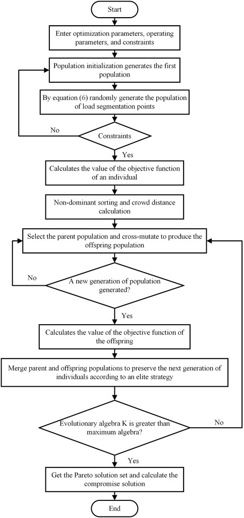
FIGURE 1. Flowchart of the adaptive segmented optimization model for the net load curve.

3.1 Objective function

The multi-objective optimization method is used to segment the net load curve, wherein the optimization objective is that the index representing the dispersion between the average values of the net loads in different periods is the largest, and the index representing the dispersion of the net loads in the same period is the smallest. If the number of segments of the net load curve is, to make the direction of the optimization target consistent, the optimization target is treated as the reciprocal, that is, the objective of the optimization segment of the net load curve is

$\{\begin{array}{l}\min f_1=\frac{1}{M_1}=\frac{1}{\max \frac{1}{N_L}{\displaystyle \sum }_{i=1}^{N_L}(P_{ave,i}-P_{ave}{)}^2},\\ \min f_2=M_2={\displaystyle \sum }_{i=1}^{N_L}\left[\frac{1}{L_i}{\displaystyle \sum }_{j=1}^{L_{\mathrm{i}}}\left(P_{Lij}-P_{ave,i}\right)\right],\end{array}(6)$

where ${\mathrm{P}}_{\mathrm{a}\mathrm{v}\mathrm{e}}$ is the average value of the load at all times; ${\mathrm{P}}_{\mathrm{a}\mathrm{v}\mathrm{e},\mathrm{i}}$ is the average net load average in the i -th segment; ${\mathrm{P}}_{\mathrm{L}\mathrm{i}\mathrm{j}}$ is the load size of the j-th load point within the i-th net load section; and ${\mathrm{L}}_{\mathrm{i}}$ is the total number of load points in the i-th segment.

3.2 Constraint condition

The net load value of each time in each subsection after the optimization subsection takes the average load value of that subsection. When the net load curve is divided into $N_L$ subsections, there are $N_L$-1 load subsections, the optimal control variable is $t_1$, $t_2$, …, $t_{N-1}$, where the load staging points cannot exceed the 24-h all-day range and the staging points can not be equal, the control variable constraint is

$\{\begin{array}{l}1\le t_i\le 24,i=\mathrm{1,2},...,N_L-1,\\ t_i\ne t_j,i\ne j.\end{array}(7)$

3.3 Model solving process

This paper is solved by the NSGA-II algorithm (Verma et al., 2021), which is usually used in the field of multi-objective optimization, which has high computational efficiency and good robustness, and the obtained pareto solution set is evenly distributed, as shown in Figure 1.

4 Considering reasonable abandon the wind net load curve adaptive piecewise double-layer optimization scheduling model

In this paper, under different time granularities, based on the optimal abandon of the wind rate of each time period, the load curve is divided reasonably to flexibly respond to load changes, and finally the start–stop and output arrangements of thermal power units are solved with the goal of minimizing the total operating cost. Therefore, a load curve adaptive subsection double optimal dispatch model considering reasonable wind abandon is constructed, and the structure diagram is shown in Figure 2.

1) The upper-layer optimization model is 5 min, 15 min, 30 min, and 1H at different time particles, with the minimum difference between the net load variance of the end power grid as the target function to optimize the wind abandonment rate in each period of time. Therefore, the optimal grid-connected power of wind power at different time granularities is obtained. At the same time, on the basis of satisfying the constraints of control variables, the net load curve after wind power grid-connected is used to solve the objective function by using NSGA-II, and the time segment points are used to obtain the step net load curve.

2) The lower-level optimization model optimizes the output of thermal power units in each period based on the stepped net load curve transmitted by the upper-level model, with the goal of minimizing the total operating cost. A number of costs are considered in the objective function, including the cost of peak shaving of thermal power units, wind power, system spinning reserve costs, and carbon transaction costs. The solver is used to obtain the optimal output, start–stop arrangement and minimum operating cost of thermal power units in the receiving end grid.

FIGURE 2

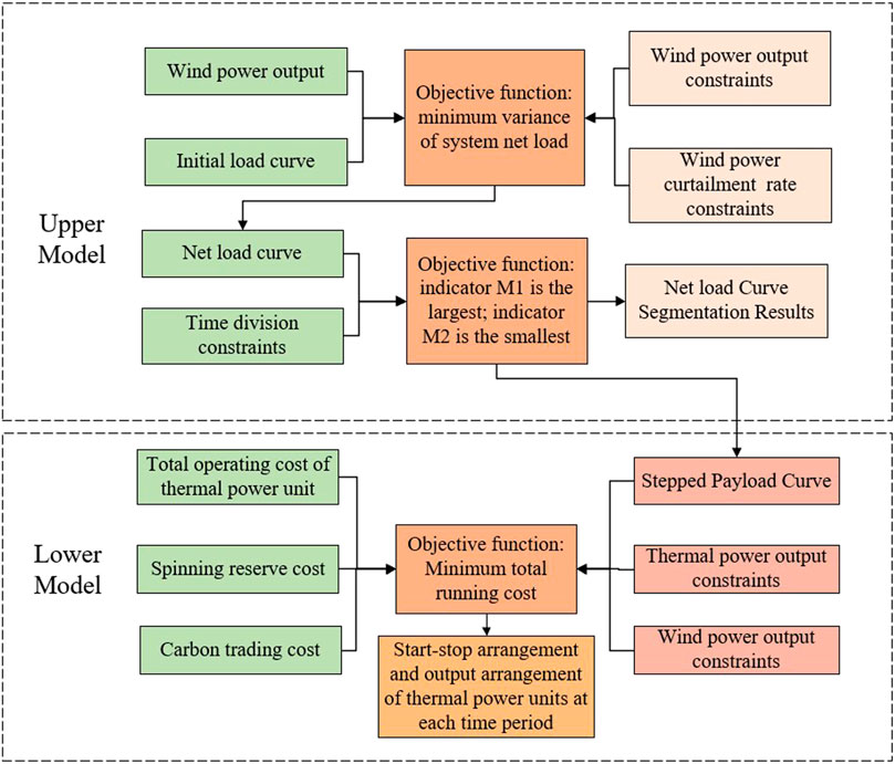
FIGURE 2. Structure diagram of the double-layer optimization mode.

4.1 Lower-layer optimization scheduling model objective function

Many costs are considered in the objective function, including the peak load regulation cost of thermal power units, system rotation standby cost, and carbon transaction cost.

$\mathit{min}{F}_2=C_1+C_2+C_3,(8)$

where ${\mathrm{F}}_2$ is the operating cost of the power grid operating for the optimization scheduling of the thermal power unit and the wind power system; ${\mathrm{C}}_1$ is the peak shaving cost; ${\mathrm{C}}_2$ is the system spinning reserve cost; and ${\mathrm{C}}_3$ is the carbon transaction cost.

1) Peak shaving cost

In the basic peak shaving stage, the peak shaving cost of the thermal power unit mainly comes from the fuel cost and the startup and shutdown costs. The calculation expression is as follows:

$C\left(P_{i,t}\right)={\displaystyle \sum }_{t=1}^T{\displaystyle \sum }_{i=1}^N\left[u_{i,t}f\left(P_{i,t}\right)+u_{i,t}\left(1-u_{i,t-1}\right)C_i^U+u_{i,t-1}\left(1-u_{i,t}\right)C_i^D\right],(9)$

$f\left(P_{i,t}\right)=a_i{P}_{i,t}^2+b_i{P}_{i,t}+c_i,(10)$

where $P_{i,t}$ is the output of thermal power unit I in period t;N is the total number of thermal power units; T is the number of periods in a scheduling period; $u_{i,t}$ is the start–stop state variable of thermal power unit i in period t, $u_{i,t}=1$, indicates that the thermal power unit I is in operation, $u_{i,t}=0,$ indicates that the thermal power unit I is in the shutdown state; $C_i^U$ is the thermal power unit i startup cost; $C_i^D$ is the thermal power unit i shutdown cost; $f\left(P_{i,t}\right)$ is the fuel cost function of thermal power unit i; and ${\mathrm{a}}_i$、 ${\mathrm{b}}_i$、 ${\mathrm{c}}_i$ are the coefficients of the consumption characteristic function of the thermal power unit i.

Linearize the coal consumption function piecewise and divide it into m segments, replacing Eq. 10 with the following equation:

$f\left(P_{i,t}\right)={\displaystyle \sum }_{s=1}^m{K}_{i,s}{P}_{i,t,s}+u_{i,t}{S}_{0,i},(11)$

$\{\begin{array}{l}{S}_{0,i}=a_i{P}_{i,\min }^2+b_i{P}_{i,\min }+c_i,\\ 0\le P_{i,t,s}\le \frac{P_{i,\max }-P_{i,\min }}{m},\\ P_{i,t}={\displaystyle \sum }_{s=1}^m{P}_{i,t,s}+P_{i,\min },\end{array}(12)$

where $K_{i,s}$ is the slope of each segment of the coal consumption function after piecewise linearization; $S_{\mathrm{0,1}}$ is the coal consumption generated by the minimum output operation of the unit after startup; and $P_{i,t,s}$ is the segmented output of the unit.

According to the output state of the unit, the peak shaving stage of the thermal power unit can usually be divided into basic peak shaving and deep peak shaving stage, and deep peak shaving can be divided into oil-feeding depth peak-shaving and non-oil-feeding depth peak shaving stage according to the peak shaving depth and combustion medium, as shown in Figure 3. Among them, $P_{\mathit{max}}$ is the maximum output of the thermal power unit, $P_{\mathit{min}}$ is the minimum output of the unit in the basic peak shaving stage, $P_n$ is the minimum output of the unit in the non-oil-feeding depth peak shaving stage, and $P_m$ is the minimum output of the unit in the peak shaving stage of the oil-feeding depth.

FIGURE 3

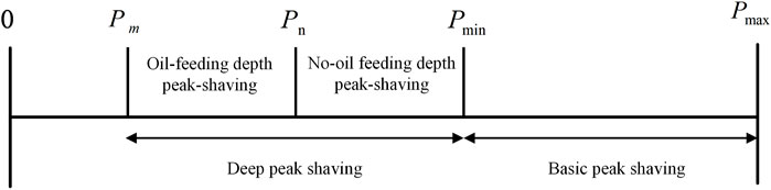
FIGURE 3. Schematic diagram of the peak shaving stage of thermal power unit.

When the unit operates at the non-oil-feeding depth peak shaving stage, the rotor metal will produce certain additional loss due to the influence of alternating stress, which will reduce the service life of the unit. The life loss cost generated during the depth of the unit peaks ${\mathrm{C}}_{\mathrm{l}\mathrm{o}\mathrm{s}\mathrm{s}}$ can be calculated as follows:

$C_{loss}={\beta }_{loss}{C}_{unit}/\left[2N_f\left(P_{i,t}\right)\right],(13)$

where ${\mathrm{C}}_{loss}$ is the life loss coefficient of thermal power unit; $C_{unit}$ is the purchase cost of thermal power unit; and $N_f\left(P_{i,t}\right)$ is the number of rotor fracturing cycles, it can be determined by the Langer formula.

During the oil-feeding depth peak shaving stage, the peak adjustment costs of the thermal power unit except for fuel costs, start–stop costs, and life loss costs, the cost $C_{oil}$ of oil investment should, the calculation formula is as follows:

$C_{oil}=P_{oil}{Q}_{oil},(14)$

where $P_{oil}$ is the oil price of the current quarter, and $Q_{oil}$ is the fuel consumption of the thermal power unit during the oil-feeding depth peak shaving stage.

To sum up, the peaking cost of thermal power units can be expressed as the following piecewise function:

$C_1=\{\begin{array}{l}C\left(P_{i,t}\right),P_{\min }\le P_{i,t}\le P_{\max },\\ C\left(P_{i,t}\right)+C_{loss},P_n\le P_{i,t}\le P_{\min },\\ C\left(P_{i,t}\right)+C_{loss}+C_{oil},P_{\mathrm{m}}\le P_{i,t}\le P_n.\end{array}(15)$

2) System spinning reserve cost

$C_2={\displaystyle \sum }_{\mathrm{t}=1}^T{\rho }_{res}\left(R_{up,load}+R_{down,load}\right),(16)$

where ${\rho }_{res}$ is the system spinning reserve cost factor; and ${\mathrm{R}}_{\mathrm{u}\mathrm{p},\mathrm{l}\mathrm{o}\mathrm{a}\mathrm{d}}$/${\mathrm{R}}_{\mathrm{d}\mathrm{o}\mathrm{w}\mathrm{n},\mathrm{l}\mathrm{o}\mathrm{a}\mathrm{d}}$ is the positive/negative rotation reserve capacity, respectively.

3) Carbon trading cost

The carbon trading mechanism restricts greenhouse gas emissions through market-based trading of carbon emission rights, which is one of the effective measures to achieve the “dual carbon” goal. At present, carbon emission trading is mainly divided into project-based trading and allowance-based trading. The project-based trading mainly refers to carrying out green development projects to achieve carbon emission reduction; quota-based carbon trading refers to the allocation of carbon emission quotas by relevant government departments to carbon emission sources. When the actual carbon emission of the emission source is higher than the allocation quota, the carbon transaction is positive, that is, the carbon emission source needs to pay a high fine to purchase carbon emission rights; and when the actual carbon emission of the emission source is lower than the allocated quota, the carbon transaction is negative; that is, carbon emission sources can sell carbon emission rights.

It can be seen from Figure 4 that the thermal power units need to purchase carbon emission allowances under the carbon trading mechanism, which will increase their operating costs and achieve the purpose of reducing carbon emissions. The sale of carbon trading quotas in the operation of wind farms will generate certain income in the grid connection, increase its grid-connected consumption, and promote the development of wind power industry. Therefore, with the improvement of the carbon trading mechanism, it can effectively promote the development of new energy power generation while reducing the carbon emissions of the power industry and promoting the development of a low-carbon economy. That is, the carbon transaction cost is calculated as follows:

$C_3=C_{\mathrm{e}}+C_w,(17)$

where $C_e$ is the thermal power unit in t time of carbon trading cost, and $C_w$ is a wind farm in t time of carbon trading cost.

1) Carbon transaction cost of thermal power unit

FIGURE 4

FIGURE 4. Carbon trading mechanism.

Thermal power units will generate a large amount of carbon dioxide during operation. After taking into account the carbon transaction cost, the excess carbon emission quota needs to be purchased in the form of transactions, which will increase the operating cost of thermal power units, which is called the carbon transaction cost of thermal power units. The calculation formula is given as follows:

$C_e=\sigma \left(Q_{et}-Q_{qt}\right),(18)$

where σ is the carbon transaction price of the thermal crew at the moment of t, yuan/t; $Q_{et}$ is the carbon emissions of thermal power units at time t, t; and $Q_{qt}$ is the carbon emission quota of thermal power units at time t, t.

The carbon emissions of thermal power units are mainly related to their output. However, due to the randomness of wind power, when the wind power is connected to the grid, to ensure the safe operation of the power grid, it is necessary to increase the rotating reserve capacity of thermal power units, which increases the carbon emissions from thermal power units. Therefore, the formula for calculating carbon emissions $Q_{et}$ of thermal power units is given as follows:

$Q_{et}={\displaystyle \sum }_{i=1}^N{l}_i\left(P_{i,t}-\lambda P_{w,t}\right),(19)$

where $l_i$ is the carbon emission intensity per unit electric capacity of thermal power unit I, t/MW; and $\lambda$ is a wind power spare capacity coefficient.

The carbon emission quota is determined according to the dispatching output of the generating unit. The calculation formula of the carbon emission quota $Q_{qt}$ of the thermal power unit is given as follows:

$Q_{qt}=\beta {\displaystyle \sum }_{i=1}^N{P}_{i,t},(20)$

where $\beta$ is the carbon trading quota per unit of electricity, t/MW.

1) Carbon transaction cost of wind farm

Wind power is a clean new energy power generation. Carbon emissions are not generated during the operation, but wind power has strong uncertainty. It will increase the rotating backup capacity of the system during the grid. The cost of increasing the mass is defined as the carbon transaction cost of wind power. The calculation formula is given as follows:

$C_w=\sigma \left(Q_{wet}-Q_{wt}\right),(21)$

where $Q_{wet}$ is the carbon emissions of the wind farm at time t, t; and $Q_{wt}$ is the carbon emissions quota of the wind farm at T, t.

$Q_{wet}={\displaystyle \sum }_{i=1}^N{l}_i{P}_{i,t}-Q_{et},(22)$

$Q_{wt}=\beta P_{w,t}.(23)$

4.2 Lower-layer optimization scheduling model constraint conditions

1) Equality constraints

The system power balance constraints:

${\displaystyle \sum }_{i=1}^N{P}_{i,t}+P_{w,t}=P_{d,t}.(24)$

2) Inequality constraints

1) Hot standby:

${\displaystyle \sum }_{i=1}^N\left(u_{i,t}{P}_{i,\max }-P_{i,t}\right)\ge \rho P_{d,t},(25)$

where $P_{i,\mathit{max}}$ is the maximum output limit of unit i; and $\rho$ is the hot standby coefficient.

2) Unit force constraint:

$u_{i,t}{P}_{i,\min }\le P_{i,t}\le u_{i,t}{P}_{i,\max },(26)$

where $P_{i,\mathit{min}}$ is the minimum output limit of unit i; and $P_{i,\mathit{max}}$ is the maximum output limit of unit i.

3) Crew climbing constraints:

$-R_u\le P_{i,t}-P_{i,t-1}\le R_u,(27)$

where ${\mathrm{R}}_{\mathrm{u}}$ is the climbing rate of the thermal power unit.

4) Unit start and stop time constraints:

$\{\begin{array}{l}\left(T_{i,t-1,off}-T_{i,off}\right)\left(u_{i,t-1}-u_{i,t}\right)\le 0,\\ \left(T_{i,t-1,on}-T_{i,on}\right)\left(u_{i,t-1}-u_{i,t}\right)\le 0,\end{array}(28)$

where $T_{i,on}/T_{i,off}$ is the minimum start/stop time of thermal power unit, respectively.

5) Start–stop cost constraints:

$\{\begin{array}{l}{C}_{i,t}^U\ge H_i\left(u_{i,t}-u_{i,t-1}\right),\\ C_{i,t}^U\ge 0,\end{array}(29)$

$\{\begin{array}{l}{C}_{i,t}^D\ge J_i\left(u_{i,t-1}-u_{i,t}\right),\\ C_{i,t}^D\ge 0,\end{array}(30)$

where $H_i$ is the single startup cost of unit i, and $J_i$ is the single shutdown cost of unit i.

6) Power flow security constraints:

$P_{L,\min }\le P_{i,t}\le P_{L,\max },(31)$

where $P_{L,\mathit{min}}$/$P_{L,\mathit{max}}$ is the minimum and maximum power flow constraints of line L, respectively.

7) Positive and negative spinning reserve constraints:

${\displaystyle \sum }_{i=1}^N\min \left(P_{i,\max }-P_{i,t}{R}_u\right)\ge r_1{P}_{w,t}+R_{up,load},(32)$

${\displaystyle \sum }_{i=1}^N\min \left(P_{i,t}-P_{i,\min }{R}_u\right)\ge r_2{P}_{w,t}+R_{down,load},(33)$

where ${\mathrm{r}}_1$/${\mathrm{r}}_2$ is the coefficient of the up/down rotation reserve capacity increased by the wind power connection, respectively, which is generally 0.1–0.2.

5 Case analysis

5.1 Example system description

In this paper, an improved IEEE -30 node system is used to simulate the power grid. The system consists of six thermal power units and one wind farm. The structure of the system is shown in Figure 5. According to the change of the typical daily load curve and wind farm law, combined with the load of the original system and the scale of wind farm, the typical daily load curve and wind power output curve of the system are simulated, as shown in Figure 6.

FIGURE 5

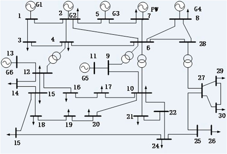
FIGURE 5. Improved IEEE-30 node system wiring diagram.

FIGURE 6

FIGURE 6. Wind power forecast output and typical daily load curve.

Parameter settings of the upper model: the rated capacity of the wind farm is 800MW, and the maximum wind abandonment rate ${\mathrm{k}}_{\mathrm{w},\max }$ is 9.8%.

The main parameters of the lower-level optimization model are shown in Table 1, and the parameters of the thermal power units are shown in Table 2.

TABLE 1

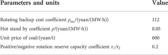
TABLE 1. Main parameters of the lower-layer model.

TABLE 2

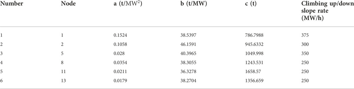
TABLE 2. IEEE-30 node system thermal power unit parameters.

5.2 Analysis before and after reasonable wind abandon

The CPLEX solver is used to solve the reasonable wind abandonment model, and the optimal wind abandonment rate at different time granularities is obtained, as shown in Figure 7. The wind power output before and after wind curtailment is shown in Figure 8, and the net load curve before and after wind curtailment is shown in Figure 9. The startup and shutdown statuses of six thermal power units are shown in Figure 10 indicates shutdown and one indicates startup. The output arrangement of the thermal power unit is shown in Figure 11.

FIGURE 7

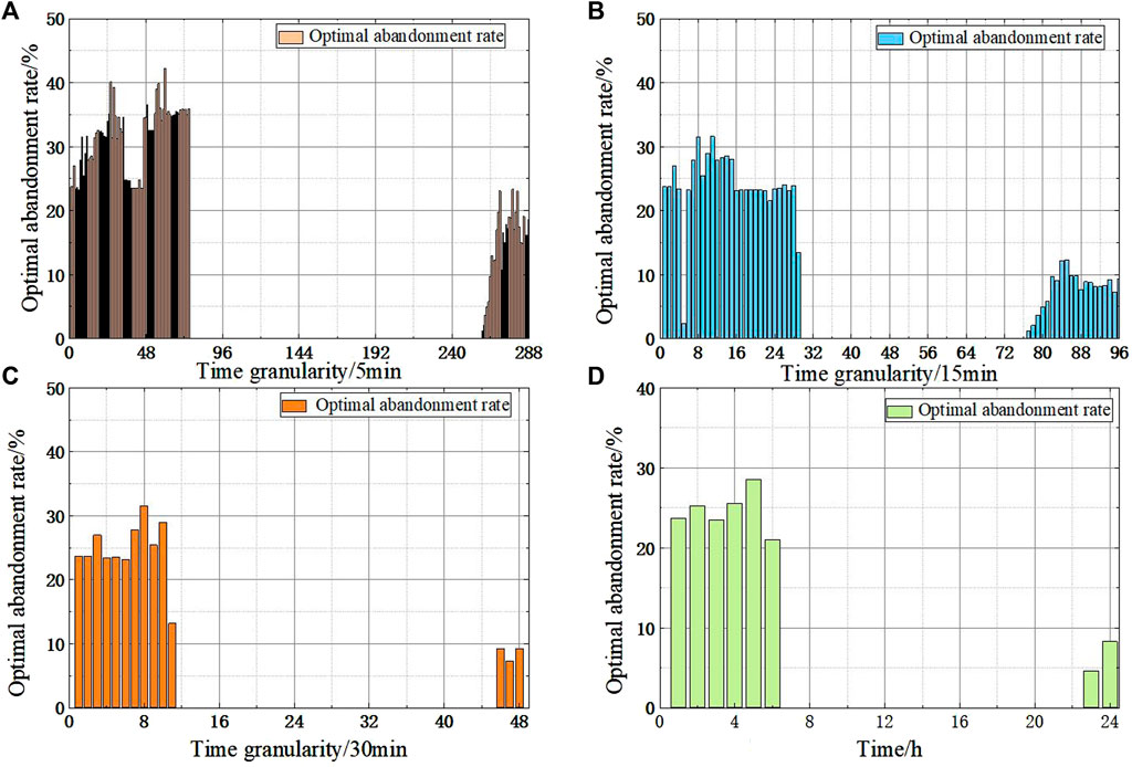
FIGURE 7. Optimal wind curtailment rate at different time granularities. (A) Curtailment rate at 5 min time granularity; (B) Curtailment rate at 15 min time granularity; (C) Curtailment rate at 30 min time granularity; (D) Curtailment rate at 1 h time granularity.

FIGURE 8

FIGURE 8. Wind power output curve before and after reasonable wind curtailment.

FIGURE 9

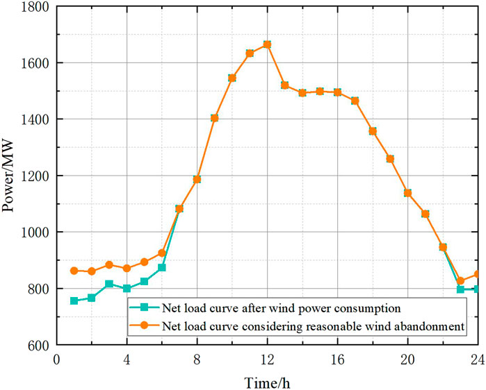
FIGURE 9. Net load curve before and after reasonable wind curtailment.

FIGURE 10

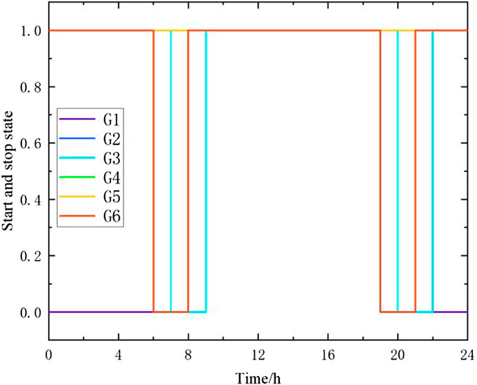
FIGURE 10. Startup and stop states of thermal power unit after reasonable abandoned wind curtailment.

FIGURE 11

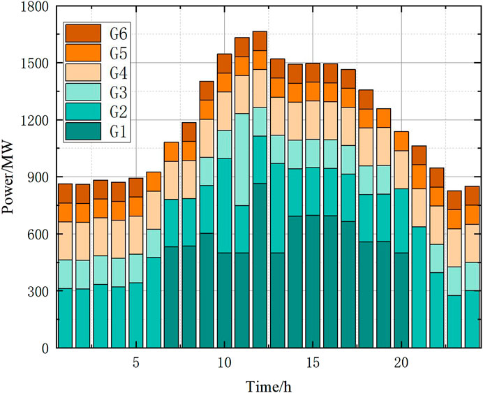
FIGURE 11. Optimal output of thermal power unit after reasonable wind curtailment.

It can be seen from Figure 7 that under different time granularities, the wind abandonment mainly occurs in the period 0:00–6:00 and 23:00–24:00. During this period, the load is relatively small, and the wind curtailment rate is maintained at a high value. The maximum wind curtailment rate reaches 28.5%, and the optimal wind curtailment rate in other periods is 0. This is related to the inverse peak regulation characteristics of the wind power and the objective function of the model. At the cost of curtailment of more wind power generation, the net load variance is guaranteed to be minimum, to obtain a relatively gentle net load curve and reduce the peak valley difference.

Comprehensive analysis of Figures 8, 9 shows that the main wind curtailment is concentrated in 0:00–7:00, the maximum peak-to-valley difference of the net load curve of all wind power consumption is 908.5MW, and after the appropriate amount of wind curtailment during the low load period, the maximum peak-to-valley difference of the net load curve is 783.8MW, a year-on-year decrease of 124.7 MW. It can be seen that considering that the reasonable wind curtailment model can significantly reduce the peak difference between the net loads, and then it can achieve the purpose of reducing the peak adjustment cost of the thermal power unit.

It can be seen from Figure 10 and Figure 11 that during the whole dispatching period, the thermal power units 2, 4, and 5 are always in the operation state, units 3 and 6 are kept in the startup state for most of the time, and unit 1 is a peak load unit. When the load is large, it is started and a relatively continuous and stable output is maintained. On the basis of ensuring the economic operation of the unit as much as possible, unit 5 shall be operated in the mode of minimum output to meet the rotating standby demand reserved due to load and wind power prediction.

From Table 3, it can be seen that the total operating cost of the system after reasonable wind curtailment is reduced by 7.27% compared with before wind curtailment, and the peak regulation cost is reduced by 6.11%, mainly because after the appropriate amount of wind curtailment during the low load period, the peak-to-valley difference and peak regulation difficulty of the load are effectively reduced, and the number of times the thermal power unit participates in deep peak shaving, resulting in a reduction in the peak shaving cost of the thermal power unit.

TABLE 3

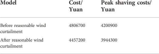
TABLE 3. Calculation results before and after wind curtailment.

5.3 Comparative analysis of different scheduling models

To verify the economy and effectiveness of the double-layer optimization model proposed in this paper under different time granularities, this paper selects four models for comparative analysis.

FIGURE 12

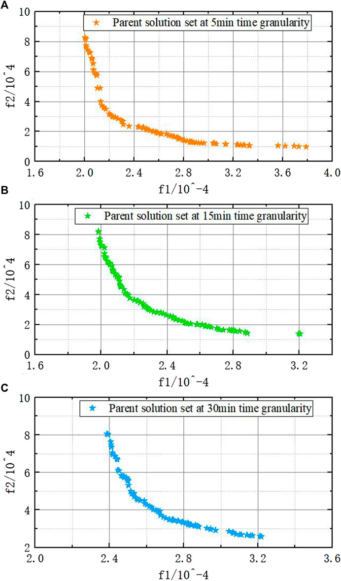
FIGURE 12. Pareto solution set under different time granularities. (A) Pareto solution set at 5 min time granularity; (B) Pareto solution set at 15 min time granularity; (C) Pareto solution set at 30 min time granularity.

FIGURE 13

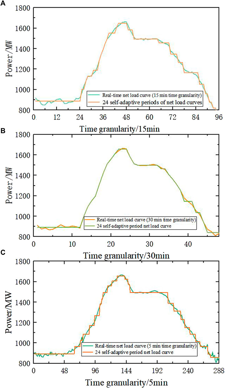
FIGURE 13. Segmentation of the net load curve under different time granularities. (A) Segmentation of net load curve at 5 min time granularity; (B) Segmentation of net load curve at 15 min time granularity; (C) Segmentation of net load curve at 30 min time granularity.

FIGURE 14

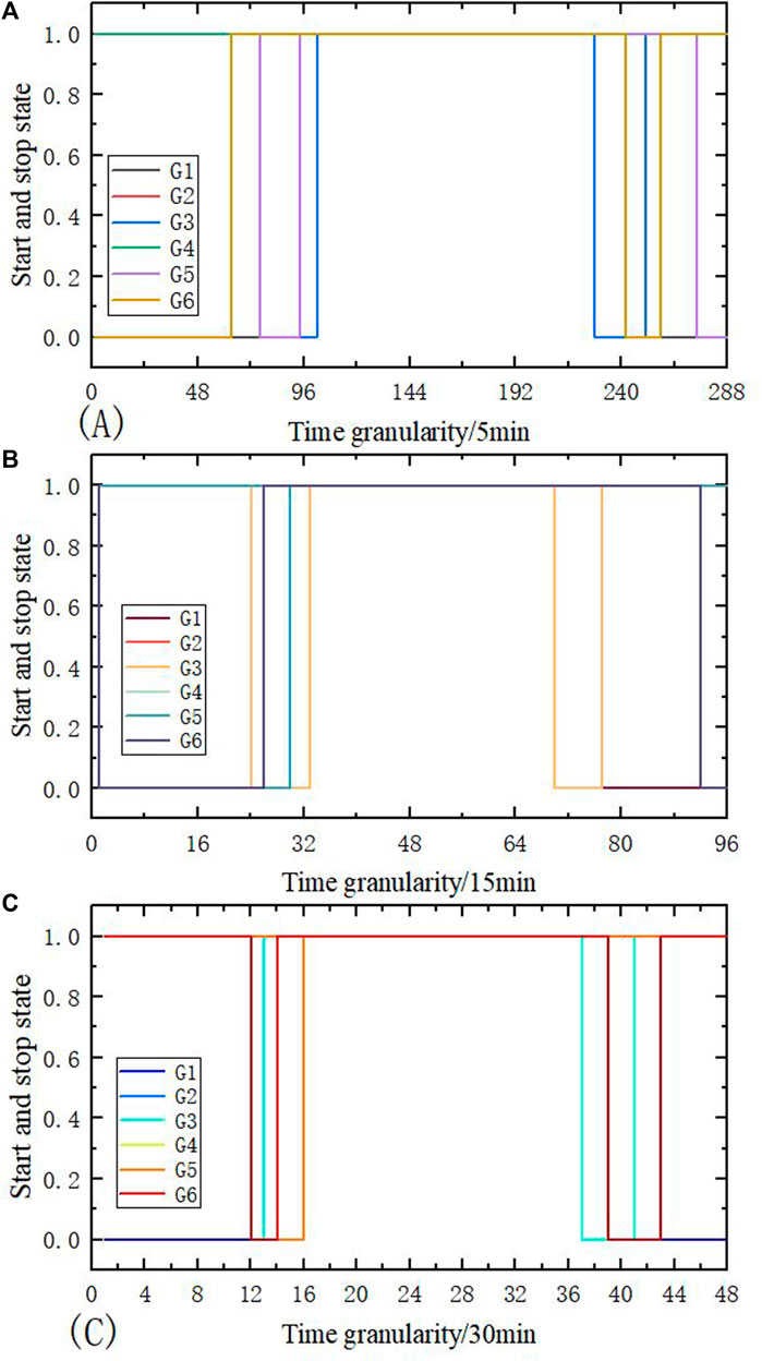
FIGURE 14. Startup and shutdown statuses of the thermal power unit under different models. (A) The start-stop state of the unit under the time granularity of 5 min; (B) The start-stop state of the unit under the time granularity of 15 min; (C) The start-stop state of the unit under the time granularity of 30 min.

FIGURE 15

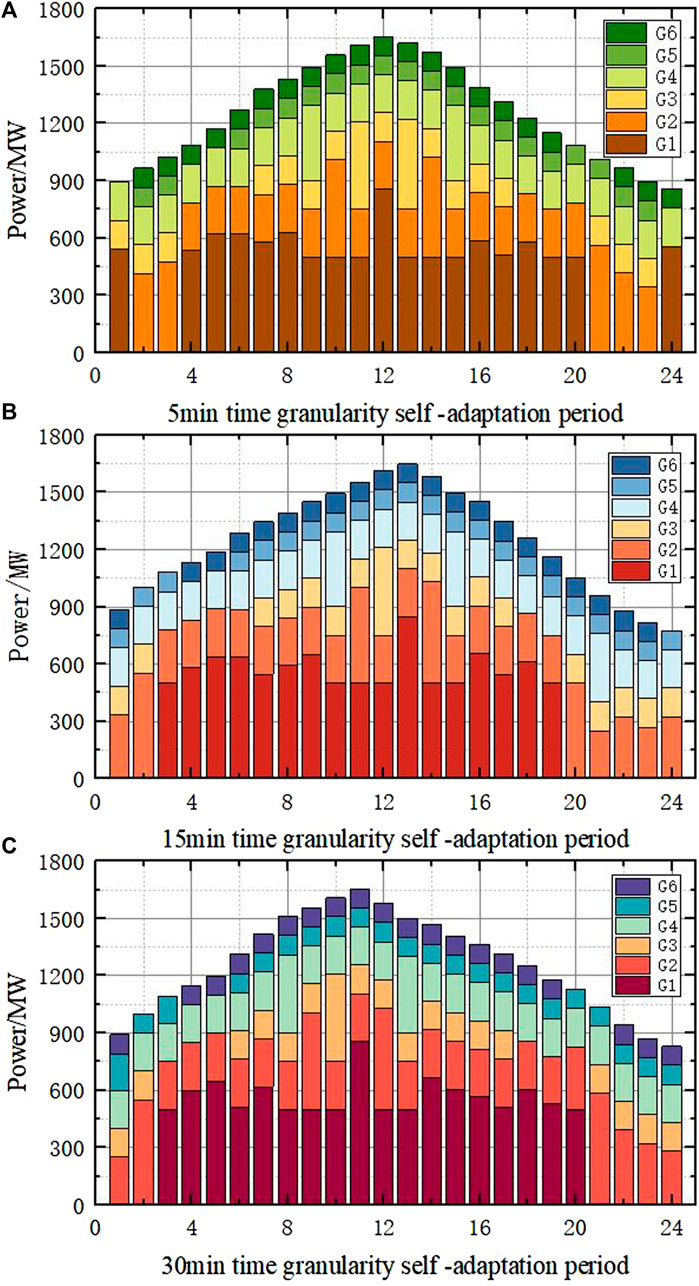
FIGURE 15. Output arrangement of the thermal power unit under different models. (A) Thermal power unit output at 5 min time granularity; (B) Thermal power unit output at 15 min time granularity; (C) Thermal power unit output at 30 min time granularity.

TABLE 4

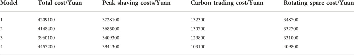
TABLE 4. Comparison of the calculation results of different models.

6 Conclusion

In this paper, the wind power grid-connected system caused by the sharp increase in peak-shaving costs and traditional scheduling is not sufficient to achieve flexible operation of the system problems; an adaptive double-layer economic dispatch model of the net load curve with reasonable exhaust air is constructed. The model makes full use of the adjustable ability of time granularity to the load gradient change and effectively responds to the net load change, while improving the wind power absorption capacity and ensuring the overall economy and environmental protection of the system. The following conclusions are obtained by the case analysis:

1) By comparing the operating results before and after the reasonable wind curtailment, the system operating cost is reduced by 7.27%, and the peak shaving cost is reduced by 6.11% compared with before wind curtailment. The calculation results show that the net load curve after the reasonable wind curtailment is relatively gentle, which can effectively avoid the deep peak shaving of the system and reduce the peak shaving cost of the system.

2) It can be seen from the analysis results that the self-adaptive subsection optimization model of the net load curve can reduce the load deviation and better deal with the random fluctuation of the net load, so that the thermal power unit has a long stable operation time and less startup and shutdown times, thus reducing the startup and shutdown costs of the unit.

3) Comparing the net load deviation and the startup and shutdown statuses of thermal power units in the dispatching cycle under different time granularities of 5 min, 15 min, 30 min, and 1h, the total operating cost of the double-layer optimal dispatching model based on 30 min time granularity is 3. 9,601 million yuan, which is 11.15% lower than that of model 4. Among them, the peak shaving cost is 535000 Yuan lower than the total consumption of wind power. The unit output arrangement is more reasonable, and the economy is better.

How to model the uncertainty of wind power and load and how to reduce curtailment using energy storage devices still need further research.

Data availability statement

The raw data supporting the conclusions of this article will be made available by the authors, without undue reservation.

Author contributions

All authors listed have made a substantial, direct, and intellectual contribution to the work and approved it for publication.

Funding

The work was supported by the Key Research and Development Plan of Shaanxi Province (2018-ZDCXL-GY-10–04), funding from the Shaanxi Province Natural Science Basic Research Program (2022JQ-534), and the National Natural Science Foundation of China Joint Fund (Key Support Project) (U1965202).

Acknowledgments

The authors would like to express their thanks to all those who have helped them over the course of researching and writing this paper. They sincerely and heartily thank and appreciate professors GZ and KZ, whose suggestions and encouragement have given them much insight into these studies. It has been a great privilege and joy to study under their guidance and supervision. Sincere gratitude also go to all the learned professors and warm-hearted teachers who have greatly helped them in their study and in life. Also, their warm gratitude goes to their friends and family who gave them much encouragement and financial support, respectively. Moreover, they wish to extend their thanks to the library and the electronic reading room for providing much useful information for the thesis.

Conflict of interest

The authors declare that the research was conducted in the absence of any commercial or financial relationships that could be construed as a potential conflict of interest.

Publisher’s note

All claims expressed in this article are solely those of the authors and do not necessarily represent those of their affiliated organizations, or those of the publisher, the editors, and the reviewers. Any product that may be evaluated in this article, or claim that may be made by its manufacturer, is not guaranteed or endorsed by the publisher.

References

Chen, G., Zhang, X., Wang, C., Zhang, Y., and Hao, S. (2021). Research on flexible control strategy of controllable large industrial loads based on multi-source data fusion of internet of things. IEEE Access 9, 117358–117377. doi:10.1109/ACCESS.2021.3105526

CrossRef Full Text | Google Scholar

Chen, Z., Hu, Y., Tai, N., Tang, X., and You, G. (2020). Transmission grid expansion planning of a high proportion renewable energy power system based on flexibility and economy. Electronics 9 (6), 966. doi:10.3390/electronics9060966

CrossRef Full Text | Google Scholar

Cheng, J., Yun, J., Zheng, Y., Zhang, Y., and Li, M. (2019). Equilibrium analysis of peak regulation right trading market between wind farms and thermal power plants considering deep peak regulation. Power Syst. Technol. 43 (08), 2702–2710. 10. 13335/j. 1000-3673. pst. 2019. 0517.

Google Scholar

Dall’Anese, E., Guggilam, S. S., Simonetto, A., Chen, Y. C., and Dhople, S. V. (2018). Optimal regulation of virtual power plants. IEEE Trans. Power Syst. 33 (2), 1868–1881. 10. 1109/TPWRS. 2017. 2741920.

Google Scholar

Deng, T., Lou, S., Xu, T., Wu, Y., and Nan, L. (2019). Optimal dispatch of power system integrated with wind power considering demand respone and deep peak regulation of thermal power units. [J].Electrical Eng. its Automation 43 (15), 34–41. (in Chinese). doi:10.7500/AEPS201806200

CrossRef Full Text | Google Scholar

Dou, C., Mi, X., Ma, K., and Xu, S. (2019). Coordinated operation of multi-energy microgrid with flexible load. J. Renew. Sustain. Energy 11 (5), 54101. doi:10.1063/1.5113927

CrossRef Full Text | Google Scholar

Gan, L. K., Zhang, P. F., Lee, J., Osborne, M. A., and Howey, D. A. (704). Data-driven energy management system with Gaussian process forecasting and MPC for interconnected microgrids. IEEE Trans. Sustain. Energy 12 (1), 695–704. doi:10.1109/TSTE.2020.3017224

CrossRef Full Text | Google Scholar

Gan, L., Hu, Y., Chen, X., Li, G., and Yu, K. (2022). Application and outlook of prospect theory applied to bounded rational power system economic decisions. IEEE Trans. Ind. Appl. 58 (3), 3227–3237. 10. 1109/TIA. 2022. 3157572.

CrossRef Full Text | Google Scholar

Guo, T., Zhu, Y., Liu, Y., Gu, C., and Liu, J. (2020). Two-stage optimal MPC for hybrid energy storage operation to enable smooth wind power integration. IET Renew. Power Gener. 14 (13), 2477–2486. doi:10.1049/iet-rpg.2019.1178

CrossRef Full Text | Google Scholar

Hao, C. A., Sna, B., Yb, B., and Fu, Y. (2021). Probability distributions for wind speed volatility characteristics:A case study of Northern Norway-ScienceDirect, Energy Reports, 7, 248–255. doi:10.1016/j.egyr.2021.07.125

CrossRef Full Text | Google Scholar

Li, Y., Cai, M., Zhou, J., and Li, Q., (2022). Accelerated multi-granularity reduction based on neighborhood rough sets. Applied Intelligence. , doi:10.1007/s10489-022-03371-0

CrossRef Full Text | Google Scholar

Liu, K., Yang, X., Fujita, H., Liu, D., and Qian, Y. (2019). An efficient selector for multi-granularity attribute reduction. Inf. Sci. 505, 457–472. doi:10.1016/j.ins.2019.07.051

CrossRef Full Text | Google Scholar

Liu, S., and Shen, J. (2022). Modeling of large-scale thermal power plants for performance prediction in deep peak shaving. Energies 15, 3171. doi:10.3390/en15093171

CrossRef Full Text | Google Scholar

Liu, Y., Liu, Q., Guan, H., Li, X., Bi, D., Guo, Y., et al. (2022). Optimization strategy of configuration and scheduling for user-side energy storage. Electronics 11 (1), 120. doi:10.3390/electronics11010120

CrossRef Full Text | Google Scholar

Liu, Y., Qiao, Y., Han, S., Xu, Y., Geng, T., and Ma, T. (2021). Quantitative evaluation methods of cluster wind power output volatility and source-load timing matching in regional power grid. Energies 14 (16), 5214doi. doi:10.3390/en14165214

CrossRef Full Text | Google Scholar

Luo, G., Zhang, X., Liu, S., Dan, E., and Guo, Y. (2019). Demand for flexibility improvement of thermal power units and accommodation of wind power under the situation of high-proportion renewable integration—Taking north hebei as an example. Environ. Sci. Pollut. Res. 26 (7), 7033–7047. doi:10.1007/s11356-019-04177-3

PubMed Abstract | CrossRef Full Text | Google Scholar

Ming, D. A., Yn, A., Bo, H. B., Zhou, G., Luo, H., and Qi, X. (2021). Frequency regulation analysis of modern power systems using start-stop peak shaving and deep peak shaving under different wind power penetrations. Int. J. Electr. Power & Energy Syst. 125, 106501. doi:10.1016/j.ijepes.2020.106501

CrossRef Full Text | Google Scholar

Mz, A., Zy, A., Wei, L. A., Yu, J., Dai, W., and Du, E. (2021). Enhancing economics of power systems through fast unit commitment with high time resolution. Appl. Energy 281, 116051. doi:10.1016/j.apenergy.2020.116051

CrossRef Full Text | Google Scholar

Ran, L. I., Fan, S., Liu, H., Ding, X., Han, Y., and Yan, J. (2020). Economic dispatch with hybrid time-scale of user-level integrated energy system considering differences in energy characteristics. Power Syst. Technol. 44 (10), 3615–3624. 10. 13335/j. 1000-3673. pst. 2020. 0420.

Google Scholar

Shi, H., Ma, Q., Smith, N., and Li, F. (2019). Data-driven uncertainty quantification and characterization for household energy demand across multiple time-scales. IEEE Trans. Smart Grid 10 (3), 3092–3102. 10. 1109/TSG. 2018. 2817567.

CrossRef Full Text | Google Scholar

Song, T., Han, X., and Zhang, B. (2021). Multi-time-scale optimal scheduling in active distribution network with voltage stability constraints. Energies 14 (21), 7107. doi:10.3390/en14217107

CrossRef Full Text | Google Scholar

Sun, Ke, MengCheng, JianLin, and Wang, Zhidong (2020). Wind fram access capacity and access location optimization method aming at minimum wind abandonment[J]. Adv. Technol. Electr. Eng. Energy 39 (08), 40–46. 10. 12067/ATEEE1905069.

Google Scholar

Tang, Z., Liu, J., and Zeng, P. (2022). A multi-timescale operation model for hybrid energy storage system in electricity markets. Int. J. Electr. Power & Energy Syst. 138, 107907. doi:10.1016/j.ijepes.2021.107907

CrossRef Full Text | Google Scholar

Verma, S., Pant, M., and Snasel, V. (2021). A comprehensive review on NSGA-II for multi-objective combinatorial optimization problems. IEEE Access 9, 57757–57791. doi:10.1109/ACCESS.2021.3070634

CrossRef Full Text | Google Scholar

Wang, J., Huo, J., Zhang, S., Teng, Y., Li, L., and Han, T. (2021). Flexibility transformation decision-making evaluation of coal-fired thermal power units deep peak shaving in China. Sustainability 13 (4), 1882. doi:10.3390/su13041882

CrossRef Full Text | Google Scholar

Wang, M., Wu, Y., Yang, M., Wang, M., and Jing, L. (2022). Dynamic economic dispatch considering transmission–distribution coordination and automatic regulation effect. IEEE Trans. Ind. Appl. 58 (3), 3164–3174. doi:10.1109/TIA.2022.3152455

CrossRef Full Text | Google Scholar

Wanlan, Shuai, Zhu, Ziwei, Li, Xuemeng, Luo, Zhijiang, Zhu, Hailong, and Zhang, Yining (2021). Source-network-load-storage” coordinated optimization operation for an integrated energy system considering wind power consumption[J]. Power Syst. Prot. Control 49 (19), 18–26. (in Chinese). doi:10.19783/j.cnki.pspc.210037

CrossRef Full Text | Google Scholar

Wei, H., Lu, Y., Yang, Y., Zhang, C., Wu, Y., Li, W., et al. (2022). Flexible operation mode of coal-fired power unit coupling with heat storage of extracted reheat steam. J. Therm. Sci. 31 (2), 436–447. doi:10.1007/s11630-022-1583-z

CrossRef Full Text | Google Scholar

Yang, B., Cao, X., Cai, Z., Yang, T., Chen, D., Gao, X., et al. (2020). Unit commitment comprehensive optimal model considering the cost of wind power curtailment and deep peak regulation of thermal unit. IEEE Access 8, 71318–71325. doi:10.1109/ACCESS.2020.2983183

CrossRef Full Text | Google Scholar

Yang, P., Ji, C., Li, P., Yu, L., Zhao, Z., Zhang, B., et al. (2021). Hierarchical multiple time scales cyber-physical modeling of demand-side resources in future electricity market. Int. J. Electr. Power & Energy Syst. 133 (12), 107184. doi:10.1016/j.ijepes.2021.107184

CrossRef Full Text | Google Scholar

Zang, Z., Yang, X., Li, Z., Yuan, Z., Xu, C., and Chen, S. (2022). Low-carbon economic scheduling of solar thermal storage considering heat storage transformation and optimal energy abandonment[J]. Power Syst. Prot. Control 50 (12), 33–43. (in Chinese). doi:10.19783/j.cnki.pspc.211405

CrossRef Full Text | Google Scholar

Zhou, Y., Li, Y., Xu, R., Feng, D., Yan, Z., Shi, Y., et al. (2021). Optimal scheduling for power system peak load regulation considering short-time startup and shutdown operations of thermal power unit. Int. J. Electr. Power & Energy Syst. 131 (11), 107012. doi:10.1016/j.ijepes.2021.107012

CrossRef Full Text | Google Scholar