Optimal energy flow in integrated heat and electricity system considering multiple dynamics

Wide promotion of combined heat and power (CHP) units necessitates the combined operation of the power and heating system. However, the dynamics and nonlinearity in integrated heat and electricity systems (IHES) remain an obstacle to efficient and accurate analysis. To handle this issue, this paper constructs an optimal energy flow (OEF) model for the coordinated operation of the IHES considering the multiple dynamics. The dynamic heating system model is formulated as a set of nonlinear partial differential and algebraic equations (PDAE). The dynamic CHP model is formulated as a set of nonlinear differential and algebraic equations (DAEs). Then, the finite difference method (FDM) is adopted to make the dynamics tractable in the OEF. On this basis, a comprehensive OEF model for IHES is proposed. Simulations in two cases verify the effectiveness of the proposed method and highlight the significance of the dynamics in IHES.

1 Introduction

Due to the increasingly severe energy crisis, the technology that can achieve higher energy utilization efficiency has attracted significant attention worldwide. The CHP unit, which co-generates the heat and electric power by recovering the waste heat, has been broadly utilized to reduce energy consumption (Ramsebner et al., 2021), (Zang et al., 2021), (Cruz et al., 2018). As a result, the power and heating systems are coupled more intensively, deriving the development of the IHES. On the one hand, the integration of the heating system provides additional flexibility for the power system because the dynamics in the heat network and load pose the energy storage property for operation (Zhang et al., 2021a). On the other hand, the intensive coupling introduces massive constraints for the power system operation because the heat power supply has priority over the electric power supply in the CHP unit. Thus, it is significant to perform a comprehensive analysis for the combined operation of the power system and heating system, thereby fully exploiting the economic potential of IHES (Shabanpour and Seifi, 2016).

To study the combined analysis in IHES, the modeling of heating system and CHP unit plays a fundamental role (Wu et al., 2016). Reference (Liu et al., 2016) firstly studied the modeling of IHES, where the static heating system model was proposed to describe the heat loss during the transmission process. The proposed static model has been widely employed in the planning (Gu et al., 2014), optimization (Sartor et al., 2014), and security analysis (Sartor et al., 2014) of IHES due to its superiority in brevity and clarity. However, such a model neglects the transmission delay of the heat power flow and is unsuitable for analysis in a large-scale system. Thus, various studies devoted their effort to accurately modeling the heating systems. A widely-used method is the node method proposed in (Palsson, 1999). In the node method, the mass flow inside a pipe is discretized into a set of small elements, and the temperature distribution along the pipe is considered as a combination of historic pipe inlet temperature (Li et al., 2016), (Zhang et al., 2022a). The node method performs better than the static model because it further considers the transmission delay of water flow. However, it suffers from the following deficiencies: 1) It is challenging to extend the node method into a heating system with the variable mass flow because the transmission delay in the node method needs to be continuously updated. Such a treatment is rather time-consuming (Dancker and Wolter, 2021). 2) The node method only focused on the relationships between the pipe inlet and outlet temperatures (Yao et al., 2021). Thus, the temperature distribution along the pipe cannot be obtained.

To address these issues, an efficient method is to formulate the energy conservation law for the mass flow infinitesimal, thereby deriving the thermal dynamics governed by PDE (Zhang et al., 2021b). However, implementing the combined analysis with PDE is challenging. Therefore, various methods have been proposed to handle the PDE and explore the dynamic heating system model for further analysis. Reference (Yao et al., 2021) adopted the FDM to discretize the PDE set, and the obtained model was verified through the OEF in the IHES at the distribution level. Since the step sizes significantly influence the numerical performance of FDM, reference (Wang et al., 2017) optimized the time and space size to make a trade-off between the modeling accuracy and complexity. In (Zhang N et al., 2022), the multiple timescales in IHES were considered. An event-triggered distributed hybrid control scheme was then proposed to guarantee secure and economic operation. On this basis, reference (Li et al., 2020) investigated the islanded and network-connected modes in IHES and developed a uniform dynamic Newton-Raphson algorithm to solve the multiple-mode energy management problem in a distributed IHES. Despite the FDM, the function transformation method is another mainstream method to solve thermal dynamics. In this regard, reference (Chen et al., 2021) transformed the PDE into the ODE in the Fourier domain. On this basis, an OEF model for IHES was developed to verify the effectiveness of the proposed method for economic analysis. However, the accuracy of the Fourier-based method depends on the number of sine components and scales with the modeling complexity. It is difficult to determine the suitable modeling accuracy for applications in different scenarios. In (Dai et al., 2019), a heat current model was further proposed using Fourier transform, and the thermal dynamics were modeled as an equivalent RLC circuit. In the proposed method, the dynamics of the heat network and load were both considered. Another type of function transformation method is the Laplace-based method in (Yang et al., 2020), where the time-frequency transformation is employed to construct the dynamic heating system model and solve the economic dispatch problem. To summarize, although great effort has been devoted to investigating the modeling and optimization of IHES, the following gaps still exist.

1) The current method mainly focused on the modeling of the heating system and proposed different solutions to the thermal dynamics. However, nonlinearity was neglected in most literature.

2) Most studies considered the coupling unit as the capacity constraint in the optimization problem, in which the physical properties and dynamics in the equipment are over-simplified, thereby influencing the practicality of the proposed work.

To overcome the deficiencies, this paper models the dynamics inside the heating system and the CHP units, with which a finite difference method is employed for numerical discretization. Also, a comprehensive OEF model is developed to investigate the coordinated operation of the IHES and explores the economic influences of heating system integration. The main contributions of this paper are summarized below.

1) We propose a complete characterization of the IHES model, including the heating system model governed by nonlinear PDAEs, the power system model governed by nonlinear algebraic equations, and the CHP unit model governed by nonlinear DAEs.

2) Based on the characterization of IHES, we develop a novel OEF model considering the dynamics and nonlinearity, where the operational and physical constraints of different components in IHES are considered.

The remainder of this paper is as follows. The IHES model considering multiple dynamics is presented in Section 2. The OEF model for IHES is developed in Section 3. The numerical simulation and conclusion are given in Section 4 and Section 5, respectively.

2 IHES model considering multiple dynamics

An IHES is a complex system containing the power system part and heating system part. The two subsystems are coupled through energy cogeneration and conversion equipment, such as CHP units and electric boilers. In this section, we firstly give the basic model of the IHES and clarify the internal dynamics, which provide the basis for OEF modeling. The structure of the IHES is shown in Figure 1.

FIGURE 1

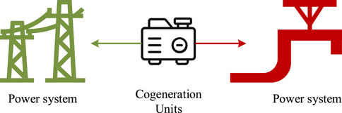
FIGURE 1. Sketch of IHES.

2.1 Heating system

The heating system is a two-layer system, including the supply and return networks. The heat power is generated at the heat sources and then transferred through the pipes in the supply network. After exchanging the heat power at consumers, the water reflows into the return work and is sent to the heat sources, thereby forcing a cycle. Since the heat power is mainly carried by the water and consumed as high-temperature water, the heating system model contains the hydraulic and thermal parts. The hydraulic part describes the mass flow rate and pressure distribution. The thermal part describes the temperature and heat power distribution (Liu et al., 2016). The explanations for the two-part model are given below.

2.1.1 Hydraulic part

Firstly, the mass flow distribution obeys mass conservation law at the nodes, which is expressed as (Liu et al., 2016):

$\mathbf{A}\mathit{m}=\mathit{d}(1)$

where A is the node-branch incidence matrix in the heating system, m is the vector of mass flow rate along the pipes, d is the vector of mass flow rate injecting into the nodes.

Secondly, the pressure distribution obeys Kirchhoff’s law in the loop, which is expressed as (Liu et al., 2016):

$\mathbf{B}\Delta \mathit{p}=\mathbf{0}(2)$

where B is the loop-branch incidence matrix in the heating system, ∆p is the vector of pipe pressure drop. The pipe pressure drop is mainly determined by the mass flow rate, which is expressed as:

$\Delta p=K{m}^2(3)$

where K is the pipe friction resistance. The elements in A and B are given below.

$\{\begin{array}{l}{a}_{ij}=\begin{array}{cc}\pm 1& \frac{\mathrm{node}i\mathrm{is}\mathrm{the}\mathrm{inlet}}{\mathrm{o}\mathrm{u}\mathrm{t}\mathrm{l}\mathrm{e}\mathrm{t}\mathrm{o}\mathrm{f}\mathrm{p}\mathrm{i}\mathrm{p}\mathrm{e}j}\end{array}\\ a_{ij}=\begin{array}{cc}0& \mathrm{n}\mathrm{o}\mathrm{d}\mathrm{e}i\mathrm{i}\mathrm{s}\mathrm{i}\mathrm{n}\mathrm{d}\mathrm{e}\mathrm{p}\mathrm{e}\mathrm{n}\mathrm{d}\mathrm{e}\mathrm{n}\mathrm{t}\mathrm{o}\mathrm{f}\mathrm{p}\mathrm{i}\mathrm{p}\mathrm{e}j\end{array}\end{array}(4)$

$\{\begin{array}{l}{b}_{ij}=\begin{array}{cc}1& \mathrm{t}\mathrm{h}\mathrm{e}\mathrm{d}\mathrm{i}\mathrm{r}\mathrm{e}\mathrm{c}\mathrm{t}\mathrm{i}\mathrm{o}\mathrm{n}\mathrm{o}\mathrm{f}\mathrm{l}\mathrm{o}\mathrm{o}\mathrm{p}i\mathrm{i}\mathrm{s}\mathrm{t}\mathrm{h}\mathrm{e}\mathrm{s}\mathrm{a}\mathrm{m}\mathrm{e}\mathrm{a}\mathrm{s}\mathrm{p}\mathrm{i}\mathrm{p}\mathrm{e}j\end{array}\\ b_{ij}=\begin{array}{cc}-1& \mathrm{t}\mathrm{h}\mathrm{e}\mathrm{d}\mathrm{i}\mathrm{r}\mathrm{e}\mathrm{c}\mathrm{t}\mathrm{i}\mathrm{o}\mathrm{n}\mathrm{o}\mathrm{f}\mathrm{l}\mathrm{o}\mathrm{o}\mathrm{p}i\mathrm{i}\mathrm{s}\mathrm{o}\mathrm{p}\mathrm{p}\mathrm{o}\mathrm{s}\mathrm{i}\mathrm{t}\mathrm{e}\mathrm{t}\mathrm{o}\mathrm{p}\mathrm{i}\mathrm{p}\mathrm{e}j\end{array}\\ b_{ij}=\begin{array}{cc}0& \mathrm{l}\mathrm{o}\mathrm{o}\mathrm{p}i\mathrm{i}\mathrm{s}\mathrm{i}\mathrm{n}\mathrm{d}\mathrm{e}\mathrm{p}\mathrm{e}\mathrm{n}\mathrm{d}\mathrm{e}\mathrm{n}\mathrm{t}\mathrm{o}\mathrm{f}\mathrm{p}\mathrm{i}\mathrm{p}\mathrm{e}j\end{array}\end{array}(5)$

2.1.2 Thermal part

Firstly, the nodes in the heating system are modeled as heat changers, which relate the mass flow rate with the temperature. The corresponding model is expressed as:

$\varphi =C_{w}d\left(T^{n,s}-T^{n,r}\right)(6)$

where C_w is the specific heat capacity of water, ϕ is the heat power, T is the temperature in the heating system, the superscript n denotes the variable at the nodes, the superscripts s and r denote the variables in the supply and return networks, respectively.

Secondly, the temperature distribution along the pipe is modeled as a function of time and space. For simplification, we neglect the thermal conduction between the adjacent flow infinitesimal since its value is sufficiently small (Palsson, 1999). On this basis, the temperature distribution along the pipe is expressed as (Yao et al., 2021):

$\frac{\partial T^p}{\partial t}+v\frac{\partial T^p}{\partial x}+\frac{v}{C_{w}m\lambda }\left(T^p-T^a\right)=0(7)$

where the superscript p denotes the variables along the pipe, v is the flow velocity, λ is the thermal resistance of the pipe, T^a is the ambient temperature.

Thirdly, the heat water flow obeys the energy conservation law at nodes, i.e., the temperature mixture equation, which is expressed as:

$T_i^n{\displaystyle \sum }_{b\in {\mathrm{\aleph }}_{s,i}}{m}_b={\displaystyle \sum }_{k\in {\mathrm{\aleph }}_{e,i}}{m}_k{T}_k^{p,o}(8)$

where T^p,o is the temperature at the pipe outlet, Tn i is the temperature at node i, ℵ_s,i is the set of pipes whose inlet is node i, ℵ_e,i is the set of pipes whose outlet is node i.

Finally, the temperature at the pipe inlet equals the temperature at the corresponding inlet node, which is expressed as:

$T_b^{p,i}=T_i^{n}b\in {\mathrm{\aleph }}_{s,i}(9)$

It should be noted that Eqs 7–9 hold both in supply and return networks since they are symmetrical.

2.2 Power system

The power system mainly adopts the AC power flow model to describe the active/reactive power and voltage distribution. The power balance at buses is expressed as:

$P_{G,i}-P_{L,i}=U_i{\displaystyle \sum }_j{U}_j\left(G_{ij}\cos {\theta }_{ij}+B_{ij}\sin {\theta }_{ij}\right)(10)$

$Q_{G,i}-Q_{L,i}=U_i{\displaystyle \sum }_j{U}_j\left(G_{ij}\sin {\theta }_{ij}-B_{ij}\cos {\theta }_{ij}\right)(11)$

where P and Q are the net active and reactive power at buses, respectively; U and θ are the voltage magnitude and phase angle, respectively; G_ij and B_ij are the conductance and susceptance between bus i and bus j, respectively. The power flow balance at branches is expressed as:

$P_{ij}=U_i{U}_j\left(G_{ij}\cos {\theta }_{ij}+B_{ij}\sin {\theta }_{ij}\right)-G_{ij}{U}_i^2(12)$

$Q_{ij}=U_i{U}_j\left(G_{ij}\sin {\theta }_{ij}-B_{ij}\cos {\theta }_{ij}\right)+B_{ij}{U}_i^2(13)$

where P_ij and Q_ij are the active and reactive power flow between bus i and bus j, respectively.

2.3 Combined heat and power units

The CHP unit is a comprehensive system composed of different subsystems. A typical structure of the CHP unit is shown in Figure 2. In the CHP units, the gas turbine consumes the fuel flow to generate the electric power and high-temperature smoke flow. The high-temperature smoke flow is then sent into the heat exchanger to heat the water. Finally, the obtained hot water is provided for the consumers in the heating system (Zhou et al., 2021).

FIGURE 2

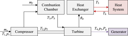
FIGURE 2. Sketch of CHP unit.

We assume that the heat loss is neglected inside the CHP unit because its value is sufficiently small. On this basis, the detailed model of the CHP unit is introduced below.

According to Figure 2, the compressor firstly consumes electric power to supercharge the air and obtain high-temperature and pressure for further processing, which is expressed as:

$p_{2,t}=CP{R}_1\times p_{1,t}(14)$

$T_{2,t}=T_{1,t}\left[1+\frac{\left(CP{R_1}^{{\beta }_1-1/{\beta }_1}-1\right)}{{\eta }_1}\right](15)$

where p₁ and p₂ are the input and output pressure of the compressor, respectively; T₁ and T₂ are the input and output temperature of the compressor, respectively; CPR₁ is the compressor ratio, β₁ is the air isentropic index, which is 1.4 in this paper; η₁ is the efficiency of the compressor, which is 0.8 in this paper (Xu et al., 2015). The electric power consumption in the compressor is expressed as:

$P_{c,t}=C_a{m}_{a,t}\left(T_{2,t}-T_{1,t}\right)(16)$

where C_a is the specific heat capacity of air, m_a is the mass flow rate of the input air. The energy balance in the combustion chamber is expressed as:

$\begin{array}{c}{\beta }_2\frac{d{T}_{3,t}}{dt}=m_{a,t}{C}_a{T}_{2,t}+m_{f,t}\left(H_{\mathrm{g}}+LHV\right)-C_s\left(m_{a,t}+m_{f,t}\right)T_{3,t}\end{array}(17)$

where β₂ is the heat storage coefficient of the combustion chamber, T₃ is the temperature in the combustion chamber, m_f is the mass flow rate of input fuel, H_g is the fuel enthalpy, LHV is the low calorific value of the input fuel, C_s is the specific heat capacity of smoke.

The temperature and pressure at the inlet and outlet in the turbine are expressed as:

$p_{3,t}=CP{R}_2{p}_{2,t}(18)$

$T_{4,t}=T_{3,t}\left[1-\left(1-CP{R_2}^{\frac{{\beta }_1-1}{{\beta }_1}}\right){\beta }_3\right](19)$

where CPR₂ is the compressor ratio in the turbine, β₃ is the smoke isentropic index, p₃ is the output pressure of the turbine, T₄ is the output temperature of the turbine. The power carried by the turbine is expressed as (Ailer et al., 2001):

$P_{b,t}=C_s\left(m_{a,t}+m_{f,t}\right)\left(T_{4,t}-T_{3,t}\right)(20)$

On this basis, the power supplied for the generator and the heat exchanger is expressed as:

$P_{g,t}={\eta }_2{\eta }_3\left(P_{b,t}-P_{c,t}\right)(21)$

${\varphi }_{g,t}={\eta }_2\left(1-{\eta }_3\right)\left(P_{b,t}-P_{c,t}\right)(22)$

where η₂ is the mechanical efficiency of the turbine, η₃ is the ratio of power supplied for the generator, P_g and ϕ_g are the supplied electric power and heat power, respectively. The energy conservation in the heat exchanger is expressed as:

${\beta }_4\frac{d{T}_{5,t}}{dt}={\varphi }_{g,t}-C_w{m}_{w,t}\left(T_{5,t}-T_{6,t}\right)(23)$

where β₄ is the heat storage coefficient of the heat exchanger, m_w is the water leaving the heat exchanger, T₅ and T₆ are the outlet and inlet temperatures of the heat exchanger. Eq. 23 indicates that the temperature change in the heat exchanger is caused by the injecting heat power and leaving heat water, T₅ and T₆ refer to the output and input temperature of the heat exchanger, respectively.

3 Optimal energy flow model in IHES

In this part, we present the optimal energy flow model in IHES. We firstly introduce the solution to the dynamics in IHES so that the corresponding ODEs and PDEs can be included in the OEF model. On this basis, we formulate the OEF model, where multiple dynamics are comprehensively considered.

3.1 Dynamics in integrated heat and electricity system

Under normal operations, the power system reaches steady-state rapidly because the electric power flow transfers at light speed. In contrast, the heat power transfers at the water flow velocity, and the corresponding processes are much longer. Thus, the dynamics in IEHS under regular operation mainly contain the thermal dynamics in the heating systems and coupling units. However, we cannot directly apply the PDE and ODE in Section 2 for optimization. Thus, the FDM is used here to discretize these equations into algebraic equations.

We adopt a second-order scheme to discretize (7) due to its superiority in convergence and stability (Yao et al., 2021). Firstly, we discretize the district (0 ≤ x ≤ L, 0 ≤ t≤Γ) with two sets of lines to obtain the differential grid in Figure 3, where N_x and N_t denote the numbers of space and time steps, respectively; ∆x and ∆t denote the space and time step sizes, respectively.

FIGURE 3

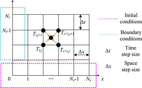
FIGURE 3. Illustration of FDM for thermal dynamics.

Expanding Eq. 7 at x = x_i+1/2, t = t_j+1/2, we can replace the differential terms with the following quotients by neglecting the high-order remainders.

$\frac{\partial T^p}{\partial x}=\frac{T_{i+1,j}^p+T_{i+1,j+1}^p-T_{i,j+1}^p-T_{i,j}^p}{2∆x}(24)$

$\frac{\partial T^p}{\partial t}=\frac{T_{i,j+1}^p+T_{i+1,j+1}^p-T_{i,j}^p-T_{i+1,j}^p}{2∆t}(25)$

$T^p=\frac{T_{i,j+1}^p+T_{i+1,j+1}^p+T_{i,j}^p+T_{i+1,j}^p}{4}(26)$

$\Delta x=\frac{L}{N_x},∆t=\frac{\mathrm{\Gamma }}{N_t}(27)$

Substituting Eqs 24–26 into Eq. 7, the temperature distribution along the pipe can be expressed with the following algebraic equations.

$T_{i+1,j+1}^p=J_1{T}_{i,j}^p+J_2{T}_{i,j+1}^p+J_3{T}_{i+1,j}^p+J_4{T}_a(28)$

$\{\begin{array}{l}{J}_1=\frac{2C_{w}m\lambda ∆x+2C_{w}m\lambda v∆t-v∆t∆x}{2C_{w}m\lambda ∆x+2C_{w}m\lambda v∆t+v∆t∆x}\\ J_2=\frac{-2C_{w}m\lambda ∆x+2C_{w}m\lambda v∆t-v∆t∆x}{2C_{w}m\lambda ∆x+2C_{w}m\lambda v∆t+v∆t∆x}\\ J_3=\frac{2C_{w}m\lambda ∆x-2C_{w}m\lambda v∆t-v∆t∆x}{2C_{w}m\lambda ∆x+2C_{w}m\lambda v∆t+v∆t∆x}\\ J_4=\frac{4v∆t∆x}{2C_{w}m\lambda ∆x+2C_{w}m\lambda v∆t+v∆t∆x}\end{array}(29)$

As for the PDE in Eqs 17, 23, we adopt the backward Euler scheme for discretization. The differential term is expressed as:

$\frac{d{T}_{3,t}}{dt}=\frac{T_{3,t}-T_{3,t-1}}{∆t}(30)$

$\frac{d{T}_{5,t}}{dt}=\frac{T_{5,t}-T_{5,t-1}}{∆t}(31)$

Substituting Eqs 30, 31 into Eqs 17, 23, we can get:

$T_{3,t}=\frac{{\beta }_2{T}_{3,t-1}+∆t\left(m_{a,t}{C}_a{T}_{2,t}+m_{f,t}\left(H_{\mathrm{g}}+LHV\right)\right)}{{\beta }_2\left(1+C_s\left(m_{a,t}+m_{f,t}\right)\right)}(32)$

$T_{5,t}=\frac{∆t{\varphi }_{g,t}+∆t{C}_w{m}_{w,t}{T}_{6,t}+{\beta }_4{T}_{5,t-1}}{{\beta }_4+C_w{m}_{w,t}∆t}(33)$

3.2 Constraints formulation

3.2.1 Constraints in power system

From the optimization view, computing the OEF in the power system with a complete AC power flow model is of a great computational burden. Thus, we adopt an improved DC power flow model to construct the constraints in the power system, where the reactive power and voltage amplitude are both considered (Yang et al., 2018). Firstly, the phase angles of different buses vary slightly in the power system at the transmission level. Thus, we can obtain the following expressions:

$\sin {\theta }_{ij}\approx {\theta }_{ij},\cos {\theta }_{ij}\approx 1-\frac{{\theta }_{ij}^2}{2}(34)$

On this basis, we can get further approximations since voltage magnitude is commonly close to 1.0 p.u.

$U_i{U}_j{\theta }_{ij}\approx {\theta }_{ij},U_i{U}_j{\theta }_{ij}^2\approx {\theta }_{ij}^2(35)$

With the above equations, the power flow model can be reformulated as (Zhang et al., 2022a):

$P_{G,i}-P_{L,i}={\displaystyle \sum }_{i,j}{P}_{ij}+{\displaystyle \sum }_{i,j}{G}_{ij}{U}_i^2(36)$

$Q_{G,i}-Q_{L,i}={\displaystyle \sum }_{i,j}{Q}_{ij}-{\displaystyle \sum }_{i,j}{B}_{ij}{U}_i^2(37)$

$P_{ij}=G_{ij}\frac{U_i^2-U_j^2}{2}-B_{ij}{\theta }_{ij}+\frac{G_{ij}}{2}\left({\theta }_{ij}^2+U_{ij}^2\right)(38)$

$Q_{ij}=B_{ij}\frac{U_j^2-U_i^2}{2}-G_{ij}{\theta }_{ij}-\frac{B_{ij}}{2}\left({\theta }_{ij}^2+U_{ij}^2\right)(39)$

During the optimization, the electric states should not only satisfy the power flow equations but also satisfy the operational constraints as follows.

$U_i^{\min }\le U_i\le U_i^{\max }(40)$

$-\frac{\pi }{2}\le {\theta }_i\le \frac{\pi }{2}(41)$

$\sqrt{P_{ij}^2+Q_{ij}^2}\le S_{ij}^{\max }(42)$

$P_{G,i}^{\min }\le P_{G,i}\le P_{G,i}^{\max }(43)$

$Q_{G,i}^{\min }\le Q_{G,i}\le Q_{G,i}^{\max }(44)$

where Eq. 40 is the voltage magnitude constraints, Eq. 41 is the phase angle constraints, Eq. 42 is the thermal constraints along the branches, Eqs 43, 44 are the active and reactive power constraints at generators.

3.2.2 Constraints in heating system

Despite the constraints in Eqs 1–3, 8–9, the OEF problem in the heating system is supposed to include the following operational constraints:

$p_i^{\min }\le p_i\le p_i^{\max }(45)$

$m_i^{\min }\le m_i\le m_i^{\max },d_i^{\min }\le d_i\le d_i^{\max }(46)$

${\gamma }^{\min }{m}_{i,t-1}\le m_{i,t}\le {\gamma }^{\max }{m}_{i,t-1},{\gamma }^{\min }{d}_{i,t-1}\le d_{i,t}\le {\gamma }^{\max }{d}_{i,t-1}(47)$

$T_{i,t}^{n,s,\min }\le T_{i,t}^{n,s}\le T_{i,t}^{n,s,\max }(48)$

$T_{i,t}^{n,r,\min }\le T_{i,t}^{n,r}\le T_{i,t}^{n,r,\max }(49)$

where Eq. 45 is the security constraint for node pressure, Eq. 46 is the capacity constraint for mass flow rate, Eq. 47 is the changing ratio constraint for mass flow rate, Eqs 48, 49 are the supply and return temperature constraints at nodes, respectively.

3.2.3 Constraints in CHP units

The CHP units combine the power system and heating system. Thus, the constraints in CHP units should firstly include the connections between different systems, which are expressed as:

$P_{g,t}=P_{G,i,t}i\in {\mathrm{\aleph }}_{\mathrm{C}\mathrm{H}\mathrm{P}}(50)$

$m_{w,t}=d_{i,t}i\in {\mathrm{\aleph }}_{\mathrm{C}\mathrm{H}\mathrm{P}}(51)$

$T_{5,t}=T_i^{n,s},T_{6,t}=T_i^{n,r}i\in {\mathrm{\aleph }}_{\mathrm{C}\mathrm{H}\mathrm{P}}(52)$

In the above equations, ℵ_CHP is the set of buses/nodes equipped with the CHP units. Eq. 50 indicates that the supplied power of the turbine in the CHP unit equals the active power generation at electric sources; Eq. 51 indicates that the injecting mass flow rate at the sources nodes equals the water flow in the heat exchanger; Eq. 52 indicates that the supply and return temperature at the sources nodes equals to the output and input temperature of the heat exchanger.

Furthermore, the constraints for the secure operation of CHP units include:

$T_1^{\min }\le T_{1,t}\le T_1^{\max }(53)$

$p_1^{\min }\le p_{1,t}\le p_1^{\max }(54)$

$m_f^{\min }\le m_{f,t}\le m_f^{\max }(55)$

$p_3^{\min }\le p_{3,t}\le p_3^{\max }(56)$

${\alpha }^{\min }{m}_{f,t}\le m_{a,t}\le {\alpha }^{\max }{m}_{f,t}(57)$

$T_3^{\min }\le T_{3,t}\le T_3^{\max }(58)$

$T_4^{\min }\le T_{4,t}\le T_4^{\max }(59)$

In the above equations, Eqs 53, 54 refer to the constraints at the input temperature and pressure of the air flow in the compressor. Eq. 55 refers to the constraints at the input fuel flow in the combustion chamber. Eqs 56, 58 refer to the constraints at the input temperature and pressure of smoke flow in the turbine. Eq. 57 refers to the relationships between the input air and fuel flows, where μ^min and μ^max refer to the minimum and maximum mixture ratio between the air flow and fuel flow. Eq. 59 refers to the constraints at the output temperature in the turbine.

3.3 Summary of the optimization model

The OEF in IHES aims to minimize the operational cost over the period Γ. The objective function of the OEF problem is formulated as:

$\min {\displaystyle \sum }_{t=1}^{N_t}\left(c_1{f}_{i,t}+c_2{g}_{j,t}\right)i\in {\mathrm{\aleph }}_{\mathrm{C}\mathrm{H}\mathrm{P}},j\in {\mathrm{\aleph }}_G(60)$

where c₁ and c₂ are the unit prices of the fuel and coals for the CHP units and the traditional generators, ℕ_G is the set of buses equipped with traditional generators, f is the function of consumed fuel regarding the electric power, g is the function of consumed coal regarding the electric power. f and g are expressed as (Yao et al., 2021):

$f_i={\mu }_{11}{P}_{G,i}^2+{\mu }_{12}{P}_{G,i}+{\mu }_{13}i\in {\mathrm{\aleph }}_{\mathrm{C}\mathrm{H}\mathrm{P}}(61)$

$g_i={\mu }_{21}{P}_{G,i}^2+{\mu }_{22}{P}_{G,i}+{\mu }_{23}i\in {\mathrm{\aleph }}_G(62)$

where μ₁₁-μ₁₃ and μ₂₁-μ₂₃ are the cost coefficients of the CHP units and generators, respectively. On this basis, the OEF model in IHES considering multiple dynamics is summarized as follows.

$\begin{array}{c}\min {\displaystyle \sum }_{t=1}^{N_t}\left(c_1{f}_{i,t}+c_2{g}_{j,t}\right)i\in {\mathrm{\aleph }}_{\mathrm{C}\mathrm{H}\mathrm{P}},j\in {\mathrm{\aleph }}_G\\ s.t.\mathrm{E}\mathrm{q}\mathrm{s}.\left(36\right)-\left(44\right)\\ \mathrm{E}\mathrm{q}\mathrm{s}.\left(1\right)-\left(3\right),\left(8\right)-\left(9\right),\left(28\right),\left(45\right)-\left(49\right)\\ \mathrm{E}\mathrm{q}\mathrm{s}.\left(14\right)-\left(16\right),\left(18\right)-\left(22\right),\left(32\right)-\left(33\right),\left(50\right)-\left(59\right)\\ \mathrm{E}\mathrm{q}\mathrm{s}.\left(61\right)-\left(62\right)\end{array}(63)$

The proposed model is a nonlinear programming problem with a quadratic objective function. In this paper, the problem is solved by the commercial software IPOPT.

4 Case studies

4.1 System description

To demonstrate the validity of the proposed IHES model and the effectiveness of the OEF method, numerical simulations are implemented in two different systems. Case 1 is a simple IHES, where a 6-bus power system and a 6-node heating system are coupled through a CHP unit. The structure of the IHES in Case 1 is shown in Figure 4A, and the detailed data can be found in (Lu et al., 2020). Case 2 is a complex IHES, where the IEEE 30-bus power system and two 51-node heating systems through 2 CHP units. The structures of the heating system and IHES in Case 2 are shown in Figures 4B,C, respectively. The detailed data of the power system and heating systems can be found in (Zhang et al., 2022b) and (Zhang et al., 2021a), respectively. All the simulations are performed on a PC with Intel i7 and 8GB RAM and coded by Matlab 2021b.

FIGURE 4

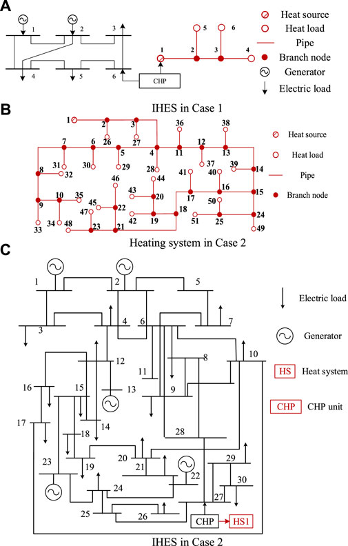
FIGURE 4. Structures of systems in case study.

4.2 Case 1

In this section, we first perform the numerical simulation of the dynamic CHP unit model to analyze the operational property of the CHP unit in IHES. The parameters of the CHP unit are acquired from (Zhou et al., 2021) and (Ailer et al., 2001) and are summarized in Table 1. The time step is 60s and the simulation period is 1 h. The response of output temperature and electric power to the input fuel flow variation is shown in Figure 5.

TABLE 1

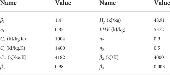
TABLE 1. Parameters of CHP unit in Case 1.

FIGURE 5

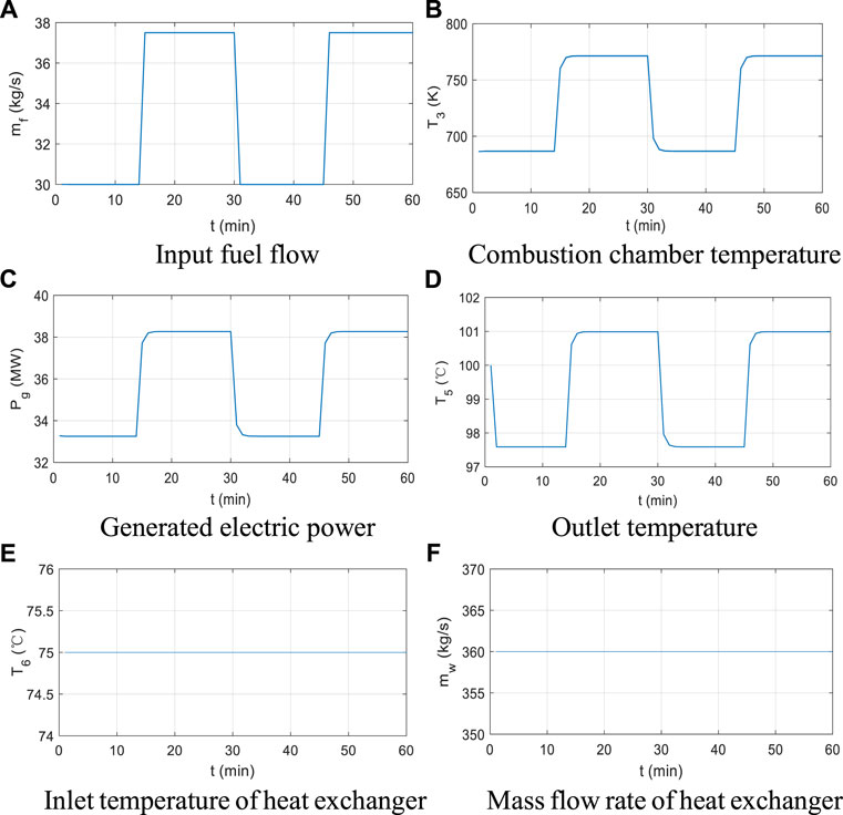
FIGURE 5. Simulation of dynamic CHP unit model.

As shown in Figure 5, the output temperature and generated electric power scales with the input mass flow rate of the fuel. However, a distinct time delay about 4min exists. Despite the capacity constraints in Eqs 21, 22, the coupling between the power and heating systems is also restricted by the pressure constraints in different components in the CHP unit, as shown in Eqs 54, 56. In this condition, the input and output states are not strictly linear, which indicates the significance of the dynamics and nonlinearity in the CHP unit model. According to Figure 5D, the initial temperature in the heat exchanger is higher and gradually decreases during the early period. As the simulation proceeds, the time-varying trend of the output temperature in the heat exchanger becomes consistent with the other states.

On this basis, we designed three scenarios to illustrate the effectiveness of the proposed method, as shown below.

S1: the proposed method with the variable hydraulic states and dynamic CHP unit model.

S2: the OEF method proposed in (Yao et al., 2021) with the fixed hydraulic states and dynamic CHP unit model. The initial conditions (hydraulic states at t = 0min) in S1 are selected as the fixed mass flow rate distribution in S2. The only difference between S1 and S2 is the adjustable mass flow rate distribution, i.e., Eqs 1–3 no longer act as constraints in S2.

S3: the proposed method without constraints in the heating system. The initial conditions in S3 are the same as that in S1. The only difference between S1 and S3 is the consideration of constraints from heating system side, i.e., Eqs 1–3, 8, 9, 32, 33, 51, 52 no longer act as constraints in S3.

The time and space steps are 15 min and 250 m, respectively. The simulation period is 4 h. The computational time and operational costs in different scenarios in Case 1 are summarized in Table 2. The optimized results are shown in Figure 6. Comparing the results in S1 and S2, we can find that the adjustable hydraulic states make the IHES more cost-effective. The savings are up to 3.3%. This is because the nonlinearity in heating system side provides more adjustable region for the operators. The operators are supposed to provide more power to heat the water flow by reducing the mass flow rate and increasing the supply temperature. The comparison between S1 and S3 indicates that the integration of the heating system will increase the cost. It is understandable because the operators need to provide more heat power to satisfy the heat consumers’ demands. Consequently, the supplied temperature and mass flow rate at the CHP unit are both increased. The differences in heating system states also influence the power system. Since the heat power provided by CHP units is the largest in S2, followed by S1, and that in S3 is the smallest. Correspondingly, the supplied electric power in S1 is the smallest due to the capacity constraints, as shown in Figure 6D.

TABLE 2

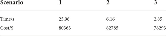
TABLE 2. Results comparison in Case 1.

FIGURE 6

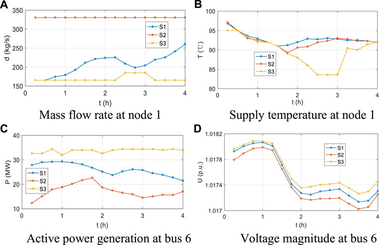
FIGURE 6. OEF results in three scenarios in Case 1.

Regarding the computational time, S3 is the most efficient because the constraints in the heating system are neglected. The computation in S1 is much more time-consuming in S2 due to the strong nonlinearity in the heating system. Nevertheless, it is still acceptable for the long time-interval dispatch.

4.3 Case 2

In this section, we extended the analysis into a larger IHES for further investigation. Three scenarios are designed for verification, including:

S1: the proposed method with the variable hydraulic states and dynamic CHP unit model.

S2: the OEF method proposed in (Yao et al., 2021) with the fixed hydraulic states and dynamic CHP unit model. The initial conditions (hydraulic states at t = 0min) in S1 are selected as the fixed mass flow rate distribution in S2. The only difference between S1 and S2 is the adjustable mass flow rate distribution, i.e., Eqs 1–3 no longer act as constraints in S2.

S3: the proposed method with the variable hydraulic states, dynamic CHP unit model, and DC power flow model. The initial conditions in S3 are the same as that in S1. The difference between S1 and S3 is the utilization of the improved DC power flow model in S1.

The time and space steps are 15 min and 100 m, respectively. The simulation period is 3 h. The computational time and operational costs in different scenarios in Case 2 are summarized in Table 3. The optimized results are shown in Figure 7. According to Table 3, the operation of IHES with adjustable hydraulic states is more cost-effective than that with fixed hydraulic states. The savings in S1 are up to 6.9%, which is two times than that in Case 1. Since the mass flow rate in Case 2 is comparatively small, the thermal loss is more distinct. The proposed method optimizes the hydraulic states to minimize the thermal loss, leading to a lower cost. Although the computational time in S1 is much larger than S2 due to the strong nonlinearity, the economic advantages brought by adjustable hydraulic states are promising. Comparing the results in S1 and S3, we can find that the OEF results in the two scenarios are almost the same, with a slight difference of 2.7%. Since the power flow nonlinearity is considered in the improved DC power flow model, S1 further considers the power flow loss in the power system. Thus, its operational cost is higher.

TABLE 3

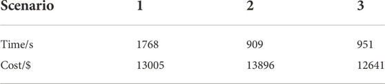
TABLE 3. Results comparison in Case 2.

FIGURE 7

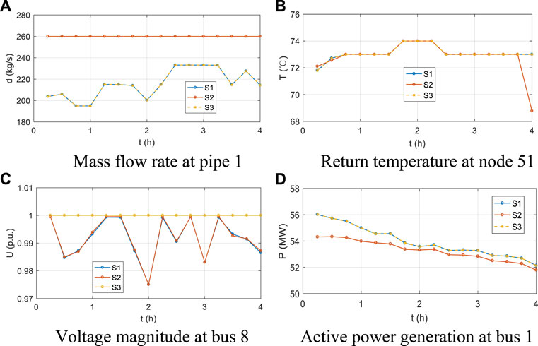
FIGURE 7. OEF results in three scenarios in Case 2.

As for the computational time, the simplification in the power system model also helps reduce the complexity. The computational time in S3 is almost half of that in S1. However, the improved DC power flow model further considers the voltage magnitude variation. As shown in Figure 7C, the maximum mismatch at bus eight is distinct, which is up to 0.223p.u. The improvement indicates the superiority of the proposed in describing the electric states accurately, which is especially significant for the operational security of IHES.

5 Conclusion

In this paper, we investigated the OEF problem for the IHES considering multiple dynamics. First, we constructed the IHES model, including the AC power flow model, dynamic heating system model, and the dynamic CHP unit model. Then, we adopted the FDM to solve the different dynamics in IHES, respectively. The heating system model governed by nonlinear PDAEs was discretized using a second-order scheme. The CHP unit model governed by nonlinear DAEs was discretized using backward Euler scheme. Finally, we constructed the OEF model for the IHES, where the dynamic property and the operational security constraints are comprehensively analyzed. Case studies verify the effectiveness of the proposed method. The numerical results indicate the significance of the nonlinearity and dynamics for the operational optimization in IHES.

In our future work, the proposed method will be extended for the analysis in the market environment.

Data availability statement

The original contributions presented in the study are included in the article/supplementary material, further inquiries can be directed to the corresponding author.

Author contributions

Conceptualization, RC; methodology and software, YL; validation and writing, KQ.

Funding

This work was supported by Science and Technology Project of State Grid Jiangsu Electric Power Company (Granted No. J2022044).

Conflict of interest

RC, YL, and KQ were employed by the State Grid Suzhou Power Supply Company.

The authors declare that this study received funding from State Grid Jiangsu Electric Power Company. The funder had the following involvement in the study: Conceptualization, Software, Methodology, Validation and Writing.

Publisher’s note

All claims expressed in this article are solely those of the authors and do not necessarily represent those of their affiliated organizations, or those of the publisher, the editors and the reviewers. Any product that may be evaluated in this article, or claim that may be made by its manufacturer, is not guaranteed or endorsed by the publisher.

References

Ailer, P., Santa, I., Szederkenyi, G., and Hangos, K. (2001). Nonlinear model-building of a low-power gas turbine. Peri. Poly. Ser. Trans. Eng. 19 (12), 117–135.

Google Scholar

Chen, Y., Guo, Q., Sun, H., and Pan, Z. (2021). Integrated heat and electricity dispatch for district heating networks with constant mass flow: A generalized phasor method. IEEE Trans. Power Syst. 36 (1), 426–437. doi:10.1109/tpwrs.2020.3008345

CrossRef Full Text | Google Scholar

Cruz, M., Fitiwi, D., Santos, S., and Catalao, J. (2018). A comprehensive survey of flexibility options for supporting the low-carbon energy future. Renew. Sustain. Energy Rev. 97, 338–353. doi:10.1016/j.rser.2018.08.028

CrossRef Full Text | Google Scholar

Dai, Y., Chen, L., Min, Y., Chen, Q., Hao, J., Fu, K., et al. (2019). Dispatch model for CHP with pipeline and building thermal energy storage considering heat transfer process. IEEE Trans. Sustain. Energy 10 (1), 192–203. doi:10.1109/tste.2018.2829536

CrossRef Full Text | Google Scholar

Dancker, J., and Wolter, M. (2021). Improved quasi-steady-state power flow calculation for district heating systems: A coupled Newton-Raphson approach. Appl. Energy 295, 120–129.

CrossRef Full Text | Google Scholar

Gu, W., Wu, Z., Bo, R., Liu, W., Zhou, G., Chen, W., et al. (2014). Modeling, planning and optimal energy management of combined cooling, heating and power microgrid: A review. Int. J. Electr. Power & Energy Syst. 54, 26–37. doi:10.1016/j.ijepes.2013.06.028

CrossRef Full Text | Google Scholar

Li, Y., Gao, D. W., Gao, W., Zhang, H., and Zhou, J. (2020). Double-mode energy management for multi-energy system via distributed dynamic event-triggered Newton-Raphson algorithm. IEEE Trans. Smart Grid 11 (6), 5339–5356. doi:10.1109/tsg.2020.3005179

CrossRef Full Text | Google Scholar

Li, Z., Wu, W., Shahidehpour, M., Wang, J., and Zhang, B. (2016). Combined heat and power dispatch considering pipeline energy storage of district heating network. IEEE Trans. Sustain. Energy 7 (1), 12–22. doi:10.1109/tste.2015.2467383

CrossRef Full Text | Google Scholar

Liu, L., Wang, D., Hou, K., Jia, H., and Li, S. (2020). Region model and application of regional integrated energy system security analysis. Appl. Energy 260, 114268. doi:10.1016/j.apenergy.2019.114268

CrossRef Full Text | Google Scholar

Liu, X., Wu, J., Jenkins, N., and Bagdanavicius, A. (2016). Combined analysis of electricity and heat networks. Appl. Energy 162, 1238–1250. doi:10.1016/j.apenergy.2015.01.102

CrossRef Full Text | Google Scholar

Lu, S., Gu, W., Meng, K., Yao, S., Liu, B., and Dong, Z. Y. (2020). Thermal inertial aggregation model for integrated energy systems. IEEE Trans. Power Syst. 35 (3), 2374–2387. doi:10.1109/tpwrs.2019.2951719

CrossRef Full Text | Google Scholar

Palsson, H. (1999). Equivalent models of district heating systems. Denmark: Technical University of Denmark.

Google Scholar

Ramsebner, J., Haas, R., Auer, H., Ajanovic, A., Gawlikm, W., Maier, C., et al. (2021). From single to multi-energy and hybrid grids: Historic growth and future vision. Rene. Sust. Energy Rev. 151, 111520.

CrossRef Full Text | Google Scholar

Sartor, K., Quoilin, S., and Dewallef, P. (2014). Simulation and optimization of a CHP biomass plant and district heating network. Appl. Energy 130 (S11), 474–483. doi:10.1016/j.apenergy.2014.01.097

CrossRef Full Text | Google Scholar

Shabanpour, A., and Seifi, A. R. (2016). An integrated steady-state operation assessment of electrical, natural gas, and district heating networks. IEEE Trans. Power Syst. 31 (5), 3636–3647. doi:10.1109/tpwrs.2015.2486819

CrossRef Full Text | Google Scholar

Wang, Y., You, S., Zhang, H., Zheng, X., Zheng, W., Miao, Q., et al. (2017). Thermal transient prediction of district heating pipeline: Optimal selection of the time and spatial steps for fast and accurate calculation. Appl. Energy 206, 900–910. doi:10.1016/j.apenergy.2017.08.061

CrossRef Full Text | Google Scholar

Wu, J., Yan, J., Jia, H., Hatziargyriou, N., Djilali, N., and Sun, H. (2016). Integrated energy systems. Appl. Energy 167, 155–157. doi:10.1016/j.apenergy.2016.02.075

CrossRef Full Text | Google Scholar

Xu, X., Jia, H., Chiang, H., Yu, D., and Wang, D. (2015). Dynamic modeling and interaction of hybrid natural gas and electricity supply system in microgrid. IEEE Trans. Power Syst. 30 (3), 1212–1221. doi:10.1109/tpwrs.2014.2343021

CrossRef Full Text | Google Scholar

Yang, J., Zhang, N., Botterud, A., and Kang, C. (2020). On an equivalent representation of the dynamics in district heating networks for combined electricity-heat operation. IEEE Trans. Power Syst. 35 (1), 560–570. doi:10.1109/tpwrs.2019.2935748

CrossRef Full Text | Google Scholar

Yang, Z., Zhong, H., Bose, A., Zheng, T., Xia, Q., and Kang, C. (2018). A Linearized OPF model with reactive power and voltage magnitude: A Pathway to Improve the MW-only DC OPF. IEEE Trans. Power Syst. 33 (2), 1734–1745. doi:10.1109/tpwrs.2017.2718551

CrossRef Full Text | Google Scholar

Yao, S., Gu, W., Lu, S., Zhou, S., Wu, Z., Pan, G., et al. (2021). Dynamic optimal energy flow in the heat and electricity integrated energy system. IEEE Trans. Sustain. Energy 12 (1), 179–190. doi:10.1109/tste.2020.2988682

CrossRef Full Text | Google Scholar

Zang, H., Xu, R., and Cheng, L. (2021). Residential load forecasting based on LSTM fusing self-attention mechanism with pooling. Energy 229, 120682.

CrossRef Full Text | Google Scholar

Zhang, N., Sun, Q., Yang, L., and Li, Y. (2022). Event-triggered distributed hybrid control scheme for the integrated energy system. IEEE Trans. Ind. Inf. 18 (2), 835–846. doi:10.1109/tii.2021.3075718

CrossRef Full Text | Google Scholar

Zhang, S., Gu, W., Lu, S., Yao, S., Zhou, S., and Chen, X. (2021). Dynamic security control in heat and electricity integrated energy system with an equivalent heating network model. IEEE Trans. Smart Grid 12 (6), 4788–4798. doi:10.1109/tsg.2021.3102057

CrossRef Full Text | Google Scholar

Zhang, S., Gu, W., Yao, S., Lu, S., Zhou, S., and Wu, Z. (2021). Partitional decoupling method for fast calculation of energy flow in a large-scale heat and electricity integrated energy system. IEEE Trans. Sustain. Energy 12 (1), 501–513. doi:10.1109/tste.2020.3008189

CrossRef Full Text | Google Scholar

Zhang, S., Gu, W., Zhang, X., Lu, H., Lu, S., Yu, R., et al. (2022a). Fully analytical model of heating networks for integrated energy systems. Appl. Energy 327, 120081. doi:10.1016/j.apenergy.2022.120081

CrossRef Full Text | Google Scholar

Zhang, S., Gu, W., Zhang, X., Lu, H., Yu, R., Qiu, H., et al. (2022b). Dynamic modeling and simulation of integrated electricity and gas systems. IEEE Trans. Smart Grid, 1. doi:10.1109/TSG.2022.3203485

CrossRef Full Text | Google Scholar

Zhou, Y., Wang, J., Dong, F., Qin, Y., Ma, Z., Ma, Y., et al. (2021). Novel flexibility evaluation of hybrid combined cooling, heating and power system with an improved operation strategy. Appl. Energy 300, 117358. doi:10.1016/j.apenergy.2021.117358

CrossRef Full Text | Google Scholar

Nomenclature

Abbreviations

CHP Combined heat and power

IHES Integrated heat and electricity system

PDAE Partial differential and algebraic equation

DAE Differential and algebraic equation

OEF Optimal energy flow

FDM Finite difference method

PDE Partial differential equation

ODE Ordinary differential equation

Indices and sets

${\mathrm{\aleph }}_{\mathrm{s},\mathrm{i}}$ Set of pipes starting at node i

${\mathrm{\aleph }}_{\mathrm{e},\mathrm{i}}$ Set of pipes ending at node i

${\mathrm{\aleph }}_{\mathrm{C}\mathrm{H}\mathrm{P}}$ Set of buses/nodes with the CHP unit

${\mathrm{\aleph }}_{\mathrm{G}}$ Set of buses with the traditional generator

min Index of the minimum values

max Index of the maximum values

Parameters

A Node-branch incidence matrix

B Loop-branch incidence matrix

K Pipe friction resistance

C_w/C_s/C_a Specific heat capacity of water/smoke/air

v Flow velocity

λ Pipe thermal resistance

γ Changing ratio of mass flow rate

T^a Ambient temperature

P_L Active power at electric load

Q_L Reactive power at electric load

G_ij Conductance between bus i and bus j

B_ij Susceptance between bus i and bus j

CPR_1-2 Compressor ratios in compressor and turbine

β₁/β₃ Air/smoke isentropic index

β₂ Heat storage coefficient of the combustion chamber

β₄ Heat storage coefficient of heat exchanger

H_g Fuel enthalpy

LHV Low calorific value

η₁ Efficiency of the compressor

η₂ Mechanical efficiency of the turbine

η₃ Energy efficiency of the turbine

N_x/N_t Number of space/time step

∆x/∆t Size of space/time step

α Mixture ratio of air and fuel

c_1-2 Price of fuel and coal

f/g Cost function of CHP unit/generator

μ Cost coefficient of CHP unit/generator

Variables

m Vector of pipe mass flow rate

d Vector of node mass flow rate

∆p Vector of pipe pressure drop

T^n,s/T^n,r Node supply/return temperature

ϕ Heat power

T^p Pipe temperature

P_G Active power at electric generator

Q_G Reactive power at electric generator

U Voltage magnitude

θ Voltage phase angle

P_ij Active power flow between bus i and bus j

Q_ij Reactive power flow between bus i and bus j

p_1-2 Input and output pressure of the compressor

p₃ Output pressure of the turbine

T_1-2 Input and output temperature of the compressor

T_3-4 Input and output temperature of the turbine

T_5-6 Input and output temperature of heat exchanger

m_a/m_f Mass flow rate of air/smoke

P_b Power carried by the turbine

P_c Power consumed by the compressor

P_g/ϕ_g Generated electric/heat power