Wind power interval prediction based on variational mode decomposition and the fast gate recurrent unit

Large-scale wind power integration is difficult due to the uncertainty of wind power, and therefore the use of conventional point prediction of wind power cannot meet the needs of power grid planning. In contrast, interval prediction is playing an increasingly important role as an effective approach because the interval can describe the uncertainty of wind power. In this study, a wind interval prediction model based on Variational Mode Decomposition (VMD) and the Fast Gate Recurrent Unit (F-GRU) optimized with an improved whale optimization algorithm (IWOA) is proposed. Firstly, the wind power series was decomposed using VMD to obtain several Intrinsic Mode Function (IMF) components. Secondly, an interval prediction model was constructed based on the lower upper bound estimation. Finally, according to the fitness function, the F-GRU parameters were optimized by IWOA, and thefinal prediction interval was obtained. Actual examples show that the method can be employed to improve the interval coverage and reduce the interval bandwidth and thus has strong practical significance.

1 Introduction

Due to the development of the global economy, energy and environmental issues are increasing. The development and utilization of renewable energy has become a research hotspot worldwide. Wind energy has received increased attention because wind power has many benefits such as cleanliness, renewability, and accessibility. Wind power generation has rapidly increased worldwide and the effect of wind power on the stability and economy of the power system is increasing.

The randomness, fluctuation, and uncertainty of wind power have a significant effect on the security, stability, and economy of the power system due to the expansion of the scale of wind power integration. Wind energy prediction is the key to solve this problem. Historical data and current wind power information are used to predict changes in the wind power generation to improve the safety, reliability, and controllability of the system.

Wind power generation is greatly influenced by wind energy. Wind energy is random and volatile in nature, and this non-stability of wind energy brings great uncertainty to wind power systems. Wind power data cannot be effectively processed with traditional signal processing methods, resulting in unsatisfactory wind power data predictions. Therefore, identifying an accurate, reasonable, and effective wind power data prediction method is of great significance Peng et al. (2021); Wang et al. (2022); Zhang S. H. et al. (2022).

1.1 Literature review

Many achievements have been made with respect to wind power prediction, but commonly point prediction is utilized. Point prediction can be used to predict the expected wind power value but does not properly address uncertainty problems, fluctuations, and the fluctuation risk and occasionally does not meet the dispatching requirements Sideratos and Hatziargyriou (2007); Foley et al. (2012); Zhang et al. (2019); Pan et al. (2021); Duan et al. (2022).

Therefore, hybrid wind power prediction methods, such as interval prediction, have been implemented. The coverage probability (to be maximized) and narrower interval bandwidth (to be minimized) are two key indexes that can be used to identify the capability of interval prediction. A higher coverage probability may lead to a wider prediction interval, whereas a wider prediction interval generally results in better coverage. Interval prediction is a type of uncertainty prediction. Methods such as the Bayesian Khosravi et al. (2011a); Yang et al. (2017, 2020b), quantile regression Ul Haque et al. (2014); Yang et al. (2020a), kernel density method Bessa et al. (2012), and Bootstrap Wan et al. (2014); Ji et al. (2015); Afshari-lgder et al. (2018) are used to construct wind power intervals. However, the high computational cost and imprecise PI of the Bayesian are disadvantageous. The quantile regression and kernel density methods depend on the results of point prediction. The performance of the Bootstrap method is excellent and it can be easily implemented, but its main disadvantage is the large computational cost. In addition, an interval construction method, that is, the lower upper bound estimation (LUBE) Khosravi et al. (2011b), was proposed in which a dual-output neural network is employed to directly construct the prediction interval.

The back propagation (BP) neural network has been applied in many scenarios because of its nonlinear fitting ability. However, many parameters of the BP neural network must be optimized. When the training data are insufficient, the model is prone to over fitting, resulting in a low generalization performance. Therefore, Huang proposed the Extreme Learning Machine (ELM) in 2004 Huang and Siew (2004). Compared with the BP network, fewer parameters must be optimized. Many scholars verified that it exhibits a good performance in many fields. In another study, the ELM was used as the prediction model and PSO was utilized to optimize the initial threshold and weight of the ELM An et al. (2021). Subsequently, the Ada-Boost algorithm was employed to fuse a series of weak predictors with a strong predictor to obtain the prediction result. Later, the ELM was introduced as basic prediction model and optimized with an intelligent optimization algorithm Wang et al. (2019); Li et al. (2021). The ELM only trains the parameters of the hidden and output layers. Although fewer parameters lead to a shorter training time, too few parameters make it difficult to obtain a smaller interval bandwidth in the field of interval prediction, which affects the prediction quality. The Fast Learning Network (FLN) proposed by Li in 2014 is similar to the ELM Li et al. (2016). It connects the input and output layers so that further relevant information can be learned from the input variables, its performance have been verified in the fields of carbon emission and silicon content prediction Ren and Long (2021); Zhao et al. (2020). The study of wind power prediction is essentially a time series forecasting problem. In recent years, a version of Recurrent Neural Network (RNN), Fast Gate Recurrent Unit (F-GRU), has developed rapidly, and it has good performance in processing time series data Chen et al. (2021); Liu et al. (2021). In this study, a prediction model F-GRU was constructed by combining the advantages of GRU and FLN based on LUBE.

With respect to the optimization method of the network parameters, a meta-heuristic intelligent optimization algorithm, Whale Optimization Algorithm (WOA), was proposed by Mirjalili and other scholars in 2016 Mirjalili and Lewis (2016). The algorithm uses the encircling strategy based on the behavior of humpback whales. Prey, random search, and spiral surround are three options that can be used to update the position of each humpback whale surrounding the prey. However, the WOA has slow convergence and easily falls into the local optimum. Many scholars have optimized this method, for example, by increasing the inertial weight and improving the convergence rate Lee and Zhuo (2021); Saafan and El-Gendy (2021); Qiu et al. (2021). Considering these shortcomings, the improved whale optimization algorithm (IWOA) was used in this study to optimize the GRU parameters to obtain a prediction interval with high accuracy and smaller bandwidth Zhang D. W. et al. (2022).

Because of the complexity and factors affecting wind power data, it is very difficult to effectively predict them with general data models. Based on data preprocessing, the wind power series is initially decomposed into stationary subseries to effectively capture the performance. Subsequently, each decomposed subseries is assigned a respective prediction. The wavelet transform (WT), empirical mode decomposition (EMD), and ensemble empirical mode decomposition (EEMD) are commonly used for the decomposition of time series data Naik et al. (2018); Devi et al. (2020); Bazionis et al. (2021); Dong et al. (2021); Meng et al. (2021); Xie et al. (2021). Variational Mode Decomposition (VMD) is a time–frequency data decomposition method, which is used to decompose a multi-component signal into multiple single-component AM and FM signals; subsequently, the original signal is decomposed into several IMF components by solving the constrained variational problem Dragomiretskiy and Zosso (2014). Based on this method, “false component” and “end effect” problems that may be encountered in the iterative process of the operation can be effectively avoided. The VMD has strong nonlinear and non-stationary signal processing capabilities. In addition, it can minimize the effects of the large fluctuation and strong nonlinearity of wind power data on the prediction results. Previously, original data were decomposed using VMD; the modal components were combined into high, medium, and low frequency; andthe improved grey wolf optimization was used to optimize the ELM parameters to predict the wind power Ding et al. (2020). In addition, a hybrid model based on a combination of a gated recurrent unit and VMD was proposed, which yielded good results Wang et al., 2020.

Based on the combination of the fast learning and generalization abilities of the FLN and the processing time serial data ability of the GRU, a new networks F-GRU is proposed in this study. In the data processing part, we use VMD to decompose, so as to enhance the extraction of useful information. Since the fitness function is non convex, IWOA algorithm is used to optimize the network parameters. Finally, we propose VMD-IWOA-F-GRU wind power interval prediction model. To verify the effectiveness of the proposed model, a wind farm in Wenchang, Hainan, China, was used as an example to build a model for experiments using MATLAB 2019b, and the results verify the capability of the proposed model.

Compared with previous wind power interval forecasting studies, this study contributes to the current understanding as follows:

1) In view of the non-stationary and nonlinear characteristics of the original wind power data, VMD was used as a preprocessing method to decompose the original data and obtain multiple single-component signals. This procedure reduces the fitting difficulties and fully utilizes the inherent data information.

2) The F-GRU were used to construct the wind power interval prediction model based on the LUBE. The results of the case analysis show that the F-GRU has a better generalization ability than the traditional BP, ELM and FLN networks.

3) Considering shortcomings of the WOA, the nonlinear convergence method was modified. The adaptive inertial weight and chaotic search were added to improve the optimization ability of the algorithm.

4) Based on the use of actual power data obtained at a wind farm, the decomposition method, optimization algorithm, and network model were compared to verify the effectiveness of the new interval prediction model proposed in this study.

1.2 Paper organization

The mathematical VMD model and IWOA are described in Section 2. The F-GRU prediction model based on LUBE is constructed in Section 3 and the new objective function is used as a fitness function to optimize the network parameters. The excellent performance of the prediction model proposed in this paper is verified in Section 4 based on the use of four seasons of real wind farm data. The conclusions are summarized in Section 5.

2 Methodology

2.1 Variational mode decomposition

The VMD of nonlinear and nonstationary signals based on the data itself is adaptive. The VMD generalize the classic Wiener filter into multiple and adaptive bands, which can realize signal adaptive decomposition by finding the optimal solution of the constraint variational model. VMD is a novel signal decomposition method that is theoretically well founded and can deal with nonlinear and non-stationary signals.

We apply VMD to wind power data which can be expressed as follow:

$S=\left\{u_1\left({\omega }_1\right),u_2\left({\omega }_2\right),\dots ,u_k\left({\omega }_k\right)\right\},k=\mathrm{1,2},\dots ,n(1)$

where u_k and ω_k are shorthand notations for the set of all modes and their center frequencies, respectively. To assess the bandwidth of a mode, we propose the following VMD scheme: 1) for each mode, compute the associated analytic signal by means of the Hilbert transform in order to obtain a unilateral frequency spectrum; 2) for each mode, shift the mode’s frequency spectrum to ‘baseband’, by mixing with an exponential tuned to the respective estimated center frequency; 3) the bandwidth is now estimated through the H¹ Gaussian smoothness of the demodulated signal, (i.e. the squared L²-norm of the gradient). The resulting constrained variational problem is as follows:

$\begin{array}{cc}\hfill & \underset{\left\{u_k\right\},\left\{{\omega }_k\right\}}{\text{min}}\left\{\sum _k{‖{\alpha }_t\left[\left(\delta \left(t\right)+\frac{j}{\pi t}\right)\ast u_k\left(t\right)\right]e^{-j{\omega }_{k}t}‖}_2^2\right\}\hfill \\ \hfill & s.t.\sum u_k=f\hfill \end{array}(2)$

To render the problem unconstrained, a quadratic penalty term and Lagrangian multipliers are employed and a new solution expression can be obtained as follows:

$\begin{array}{cc}\hfill \mathcal{L}\left(\left\{u_k\right\},\left\{{\omega }_k\right\},\lambda \right)& =\alpha \sum _k{‖{\alpha }_t\left[\left(\delta \left(t\right)+\frac{j}{\pi t}\right)\ast u_k\left(t\right)\right]e^{-j{\omega }_{k}t}‖}_2^2\hfill \\ \hfill & +{‖f\left(t\right)-\sum _k{u}_k\left(t\right)‖}_2^2\hfill \\ \hfill & +⟨\lambda \left(t\right),f\left(t\right)-\sum _k{u}_k\left(t\right)⟩\hfill \end{array}(3)$

where α is the data-fidelity constraint parameter and λ is the Lagrangian multiplier.

The alternate direction method of multipliers (ADMM) approach is used to produce different decomposed modes and the center frequency during each shifting operation. Then, the modes u_k and their corresponding center frequency ω_k can be updated as

$u_k^{n+1}\leftarrow \underset{u_k}{\text{arg}\hspace{0.17em}\text{min}}L\left(u_{i<k}^{n+1},u_{i\ge k}^{n+1},{\omega }_i^n,{\lambda }^n\right)(4)$

and

${\omega }_k^{n+1}\leftarrow \underset{{\omega }_k}{\text{arg}\hspace{0.17em}\text{min}}L\left(u_i^{n+1},u_{i<k}^{n+1},{\omega }_{i\ge k}^n,{\lambda }^n\right)(5)$

Each mode obtained from solutions in the spectral domain can be represented as

${\widehat{u}}_k\left(\omega \right)=\frac{\widehat{f}\left(\omega \right)-{\sum }_{i\ne k}{\widehat{u}}_i\left(\omega \right)+\left(\widehat{\lambda }\left(\omega \right)/2\right)}{1+2\alpha {\left(\omega -{\omega }_k\right)}^2}(6)$

2.2 Improved whale optimization algorithm

The whale optimization algorithm (WOA) is a global random searching method based on swarm intelligence, which was inspired by the specific hunting behavior of the humpback whales. The mathematical modeling of the behavior of whale optimization algorithm consists of three phases: random search, encircling prey and bubble-net attacking. As a swarm intelligence algorithm, WOA has the disadvantages of slow convergence speed and easy to fall into local optimization, which seriously affects the speed and accuracy of data processing. In this paper, the non-negative convergence factor and adaptive inertial weight are introduced into the whale optimization algorithm to overcome the convergence problem, which can converge quickly. The adaptive chaotic search is introduced to improve the ability to jump out of local optimum.

2.2.1 Non-linear convergence factor

To overcome the convergence problem and optimization out of balance, we introduce the non-linear convergence factor α, which determines the step length of the whale approaching the optimal individual. The convergence factor α decreases nonlinearly with the increase of the number of iterations. In the initial stage, the attenuation degree of α is low, and the whale can move in a larger stride to better find the global optimal solution. In the later stage, the attenuation degree of α increases and the moving stride of whales decreases, so the optimal solution can be found more accurately. Thus, the development ability of global search and the mining ability of local search are more effectively balanced. The nonlinear convergence factor is defined as:

$\alpha ={\alpha }_{\max }-\frac{{\alpha }_{\max }}{1+\text{exp}\left(-\frac{T_1\left(t-T_2{t}_{\max }\right)}{t_{\max }}\right)}+{\alpha }_{\min }(7)$

Where T₁ and T₂ are non-negative constant that used to control the time of α decrease.

2.2.2 Adaptive inertial weight

As the most important parameter in particle swarm optimization algorithm, inertial weight should be a large value at the beginning of training to search the global optimization, and it should be a small value to improve the optimization accuracy when around the global optimum as the number of iterations increase. However, the decreasing trend of inertial weight affects the convergence results and diversity of the population. The slow and rapid decreasing of inertial weight will lead to the population difficult to converge and the decrease of population diversity, respectively; In order to solve the above problems, we proposed a new inertial weight that varies according to fitness of whale individual. The adaptive inertial weight can be written as:

$w=\mathrm{n}\mathrm{o}\mathrm{r}\mathrm{m}\mathrm{r}\mathrm{n}\mathrm{d}\left(1,{\sigma }^2\right)(8)$

${\sigma }^2=\frac{1}{1+{\mathrm{e}}^{2-\left(\frac{f_i-f_{\min }}{f_{\max }-f_{\min }}\times 4\right)}}(9)$

where normrnd (1,σ²) is a normal distribution with mean 0 and variance σ²; f_i is the fintess of x_i; f_max and f_min are the maximum and minimum fitness in the contemporary pupulation, respectively.

The inertial weight proposed is calculated according to the current individual fitness. For individuals with poor fitness, there is a certain probability that a large inertial weight will be used for a large-scale search, while for individuals with better fitness, a local search will be performed around the global optimum. The position update formula of whale optimization algorithm is based on the optimal whale individual in whale optimization algorithm, so the inertial weight w is added to the optimal whale individual. The position update formula after adding the adaptive inertial weight is written as:

$x\left(t+1\right)=w{x}_{\mathit{best}}-AD(10)$

$x\left(t+1\right)=D^{\prime }{\mathrm{e}}^{bl}\text{cos}\left(2\pi l\right)+w{x}_{\mathit{best}}\left(t\right)(11)$

2.2.3 Adaptive chaos search strategy

Chaos search strategy has strong randomness, which can be used to improve population diversity of the whale optimization algorithm so that whales can reduce the probability of sinking into local optimal solution caused by premature phenomena.

Tent map has the characteristic of traversing more uniformly than logistic map. In this paper an adaptive chaos search strategy is proposed to improve the search ability through uses tent map and adaptive search probability. The specific implementation method is as follows:

1) Chaos Search Strategy

The tent map function expression is:

$x_{n+1}=\left\{\begin{array}{cc}\frac{x_n}{\mu },\hfill & x_n\in \left[0,\mu \right)\hfill \\ \frac{1-x_n}{1-\mu },\hfill & x_n\in \left[\mu ,1\right]\hfill \end{array}\right.(12)$

The random search mechanism is modified as follows:

$x_i\left(t+1\right)=x_c\left(t\right)-FAD(13)$

$D=\left|C{x}_c\left(t\right)-x_i\left(t\right)\right|(14)$

where x_c is a chaos individual; F is called search factor which is used to increase the step length so that the individual whale can get rid of the local optimum. Before the start of the iteration, x_c is randomly generated which searches in the solution space by tent map. When the current whale individual executes adaptive chaotic search strategy, it will close to x_c rather than randomly selected individual, thereby increasing the diversity of population and effectively improving the optimization ability of algorithm.

2) Adaptively Adjust the Search Probability

In overcoming the premature phenomenon of the original whale optimization algorithm, we use adaptive search probability to improve the possibility of jumping out of the local optimum, which can be calculated as:

$P_c={\left(\frac{f_i-f_{\min }}{f_{\max }-f_{\min }}\right)}^k(15)$

where k is called probability factor which is used to adjust the threshold of search probability; f_i is the fitness of x_i; f_min and f_max are the minimum fitness and maximum fitness in the contemporary population, respectively. The value of P_c is related to the fitness of whale individual, it means that the high-quality whale individuals can search for better solution around current optimal solution with greater probability, while poor individuals are more likely to follow the chaotic individual x_c.

3 Interval prediction model

3.1 Network model

The lower upper bound estimation method (LUBE) is a nonparametric method that constructs the prediction interval directly. FLN is a novel artificial neural network. Since the weight from the input layer to the hidden layer is generated randomly and will not change during the training, it has a fast learning speed, and Figure 1A shows the model of FLN. GRU and LSTM are the improved neural network of RNN, both of them have better performance in processing time series related data. Compared with LSTM, fewer parameters need to be updated in GRU, and the GRU is shown in Figure 1B. Based on the advantages of both networks, we constructed the F-GRU network based on LUBE in this paper. Figure 1C shows the mode of F-GRU based on LUBE, and the mathematical modelling of the F-GRU can be represented as follows:

$\begin{array}{cc}\hfill z_t& =\sigma \left(W_z\cdot \left[h_{t-1},x_t\right]+b_z\right)\hfill \\ \hfill r_t& =\sigma \left(W_r\cdot \left[h_{t-1},x_t\right]+b_r\right)\hfill \\ \hfill \widetilde{h_t}& =\mathrm{t}\mathrm{a}\mathrm{n}\mathrm{H}\left({\text{W}}_{\text{h}}\cdot \left[{\text{h}}_{\text{t}-1}\odot {\text{r}}_{\text{t}},{\text{x}}_{\text{t}}\right]+{\text{b}}_{\text{h}}\right)\hfill \\ \hfill h_t& =\left(1-z_t\right)\odot h_{t-1}+z_t\cdot \widetilde{h_t}\hfill \\ \hfill y_U& =\sum _{j=1}^m{w}_{j1}\cdot h_{jT}+\sum _{i=1}^T{w}_{i1}\cdot x_i+b_1\hfill \\ \hfill y_L& =\sum _{j=1}^m{w}_{j2}\cdot h_{jT}+\sum _{i=1}^T{w}_{i2}\cdot x_i+b_2\hfill \end{array}(16)$

where W_z, W_r, W_h and b_z, b_r, b_h are the weight matrix and bias parameters of the update gate layer, the reset gate and candidate state, respectively; w_jo and w_io (o = 1, 2) are the weight matrix from hidden layer neurons and input layer neurons to output layer neurons, respectively; b_o (o = 1, 2) are the bias parameters of the output neurons, and it is worth noting that the parameters (W_z, W_r, W_h, b_z, b_r and b_h) in GRU are generated randomly and will not update during training, the only parameters to be trained are w_jo and w_io (o = 1, 2); σ and tanH represent the Sigmoid activation function adn tanH activation function, respectively; x_i is the input vector; y_U and y_L are the upper and lower bounds of model output respectively.

FIGURE 1

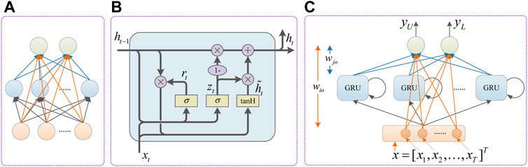
FIGURE 1. The model of F-GRU based on LUBE. (A) FLN. (B) GRU. (C) F-GRU.

3.2 Objective function for prediction interval

In the method of this paper, the quality of PI is evaluated by different performance measures, such as PI coverage probability (PICP), PI normalized root-mean-square width (PINRW), coverage width criterion (CWC) and PI average deviation. To evaluate the accuracy of the interval, the predict interval coverage probability (PICP) is introduced, PICP is defined as follows:

$PICP=\frac{1}{N}\sum _{i=1}^N{c}_i(17)$

$c_i=\left\{\begin{array}{cc}0,\hfill & y_i\notin \left[y_U,y_L\right]\hfill \\ 1,\hfill & y_i\in \left[y_U,y_L\right]\hfill \end{array}\right.(18)$

where N is the total number of prediction points; y_i is actual power value. When y_i is in the interval [y_U, y_L], the prediction interval can cover the actual value.

PINRW is defined to indicate the PIs average bandwidth and can be expressed as:

$PINRW=\frac{1}{N}\sqrt{\frac{1}{R}\sum _{i=1}^N{\left(y_U-y_L\right)}^2}(19)$

where R is the range of the actual value, which is used to normalize the average bandwidth. Moreover, PINRW ∈ [0, 1], where a smaller PINRW indicates a higher quality, and a higher PINRW indicates a lower quality.

In practice overall quality of PIs can be evaluated using coverage width-based criterion (CWC) and can be mathematically represented as:

$CWC=PINRW\left[1+\gamma \left(PICP\right){\mathrm{e}}^{-\eta \left(PICP-\mu \right)}\right](20)$

$\gamma \left(PICP\right)=\left\{\begin{array}{cc}0,\hfill & PICP\ge \mu \hfill \\ 1,\hfill & PICP<\mu \hfill \end{array}\right.(21)$

where μ is the predetermined confidence degree; η is the penalty coefficient when the PICP is less than μ.

CWC can transform complex multi-objective problems into single-objective problems effectively. However, when the upper and lower bounds coincide, the optimization result is erroneous, and the degree of the deviation of the actual value within the prediction interval is not considered. For this problem, the prediction interval average deviation (PIAD) is considered Khosravi et al. (2011b); Zhang et al. (2022a), and can be represented as:

$PIAD=\frac{1}{N}\sum _{i=1}^N\left|\frac{y_U-y_L}{2}-y_i\right|(22)$

$F=\gamma \left(PICP\right){\mathrm{e}}^{-{\eta }_1\left(PICP-\mu \right)}+PINRW+{\eta }_{2}PIAD(23)$

where η₁ is the penalty coefficient when PICP is less than μ; η₂ is the penalty coefficient for the deviation of the actual value from the center of the prediction interval. The penalty cost is high when PICP$<\mu$, which is discarded due to the larger penalty coefficient η₁ during the training process. Otherwise, the PINRW and PIAD are considered to meet the minimum target. Moreover, the known training information is fully utilized to acquire a narrower interval.

3.3 VMD-IWOA-F-GRU interval prediction framework

The VMD-IWOA-F-GRU model framework proposed in this paper is shown in Figure 2, and the whole process is described as follows:

1) Data preprocessing and construct the dataset: The outage points are removed, and than the remaining datas are decomposed with VMD. Each layer input vector x = [x_IMFK1, x_IMFK2, … , x_IMFK5] is determined, where x_IMFK1 is the wind power at the first point before the forecasting of the point in IMFK, x_IMFK2 is the wind power at the second point before the forecasting of the point in IMFK, and so forth.

2) Construct the interval prediction model: Determing the number of neurons in the hidden layer, and the parameters (W_z, W_r, W_h and b_z, b_r, b_h) are then randomly generated.

3) Optimize the prediction model: The training dataset is used as input for the prediction model and the IWOA is used to optimize the parameters of the model based on the fitness function (Eq. 23).

4) Calculate the prediction interval: By repeating the independent calculations, the model with the best evaluation metrics is selected to compose the final prediction model and tested on the test set.

5) Analysis: Evaluate and analyze according to the calculated prediction interval.

FIGURE 2

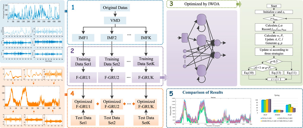
FIGURE 2. The structure of VMD-IWOA-F-GRU.

4 Example analysis

We compared the network models, optimization algorithms, and decomposition methods. Codes were developed in MATLAB 2019b and executed on an Intel core i5 CPU 6300H 2.3 GHz, 8 GB RAM processor. Seven prediction models WOA-BP, WOA-ELM, WOA-F-GRU, IWOA-F-GRU, EMD-IWOA-F-GRU, EEMD-IWOA-F-GRU and VMD-IWOA-F-GRU were independently run ten times and the best parameters were applied to the test dataset. The number of iterations is 300, the size of population is 50, and the penalty coefficients η₁ and η₂ of the objective function F are 100 and 0.2, respectively.

For models that do not use decomposition methods, such as WOA-BP, WOA-ELM, WOA-F-GRU, and IWOA-F-GRU, the ReLU function was used as the activation function. For models including decomposition methods, such as EMD-IWOA-F-GRU, EEMD-IWOA-F-GRU, and VMD-IWOA-F-GRU, the trend mode (the first IMF of VMD, the last IMF of EMD and EEMD) uses the ReLU activation function and the rest of the IMF use the tanH activation function in the output layer.

4.1 Data description

In this study, we used data measured at an existing wind farm in Wenchang, Hainan, China to verify the effectiveness of proposed interval prediction model. Each data point represents the average wind power within 10 minutes. In this study, 5,000 data points obtained in each of the four seasons were selected; 90% of the data were used as the training dataset and 10% were used as the test dataset. Figure 3 shows the time series of wind power data for four seasons.

FIGURE 3

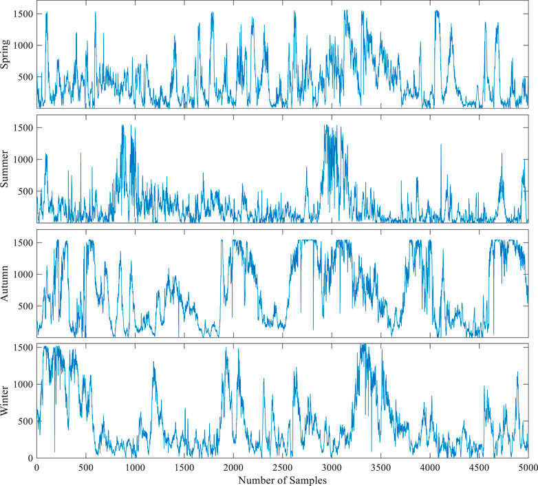
FIGURE 3. Time series of wind power data for four seasons.

4.2 Data processing

Actual wind power time series have a certain random volatility and must be de-noised. Actual power time series are complex due to the complex wind turbine, which is affected by many cross-impact loads. It is difficult to accurately analyze the data characteristics based on the graph alone and thus the time series must be decomposed. The VMD is suitable for processing nonlinear and non-stationary signals. The VMD generalizes the classic Wiener filter into multiple and adaptive bands, which realize signal adaptive decomposition by finding the optimal solution for the constraint variational model. To verify the effect of VMD, wind power data recorded in winter were used as an example. The results of VMD and those of EMD and EEMD were compared. The results are shown in Figures 4, 5.

FIGURE 4

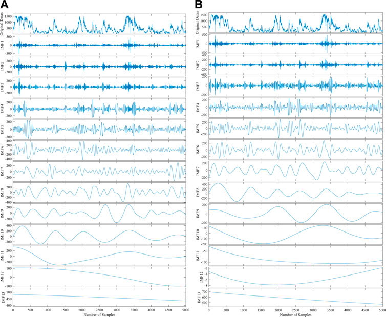
FIGURE 4. Results of the EMD and EEMD decompositions of winter data. (A) EMD decomposition results of winter. (B) EEMD decomposition results of winter.

FIGURE 5

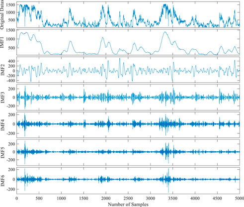
FIGURE 5. VMD decomposition results of winter.

Figure 4 shows that the mode mixing problem of EMD still exists when it is applied to composite wind power data. Hardly any completed sub-signal has been successfully decomposed. To some extent, EEMD effectively suppresses the mode aliasing, but it is difficult to assign each mode to its real physical meaning. In contrast to EMD and EEMD, VMD can be used to adaptively decompose wind power data into an ensemble of band-limited intrinsic mode functions and is suitable for the decomposition of nonlinear and non-stationary signals. The Gauss noise is removed by applying a Wiener filter to each mode during the decomposition progress. The result of VMD is shown in Figure 5. The IMF1 clearly reflects the time change of wind power data and IMF2–IMF6 reflect the changes of the wind power data in different central frequency ranges with time, which has physical significance. The VMD is more suitable for the decomposition of original wind power data than EMD and EEMD. In this study, we used VMD to decompose wind power data for preprocessing purposes.

The VMD is used to decompose the data, which helps to highlight the local characteristics of the original data and reduces the randomness and volatility of the data. The selection of the data decomposition level K significantly affects the data decomposition performance. If the K value is too low, the decomposition is insufficient. In contrast, a K value that is too high will lead to the over decomposition of the signal. In this study, the K value was determined with the central frequency analysis method. Any ten groups of data from each season were decomposed and the mean value of the center frequency was calculated, as shown in Tables 1–4.

TABLE 1

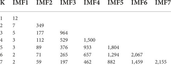
TABLE 1. Center frequencies corresponding to different K values in spring.

TABLE 2

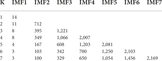
TABLE 2. Center frequencies corresponding to different K values in summer.

TABLE 3

TABLE 3. Center frequencies corresponding to different K values in autumn.

TABLE 4

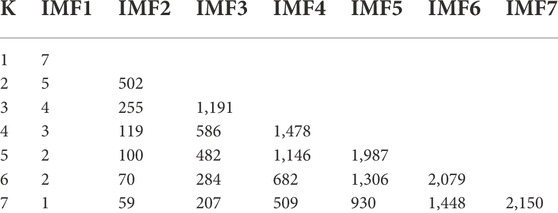
TABLE 4. Center frequencies corresponding to different K values in winter.

The inflection point of the maximum central frequency is reached in spring, autumn, and summer when K = 6. The magnitude of the change of the maximum value of the central frequency gradually decreases. In summer, the inflection point occurs when K = 4, but the results of several experiments showed that the prediction quality does not decrease when K = 6. Therefore, to unify the model, a K value of six was used in this study. The winter data were decomposed with K = 6 and VMD. The moderate bandwidth constraint α was 2000 and the tolerance range of the convergence criterion was 10^–7.

4.3 Comparison of network models and algorithms

To reveal the effectiveness of the F-GRU model for PI construction, the BP, ELM and FLN networks were compared with the F-GRU at the 90% confidence level, without decomposition. In this paper, the sample set is constructed using the values of the first five moments to predict the values of the next moment, so the number of input neurons is five in the BP, ELM and FLN networks. The number of neurons in the hidden layer is 9, and the number of neurons in the output layer is 2. Therefore, the number of parameters to be trained is 74, 20 and 30 in BP, ELM and FLN, respectively. For the F-GRU network, the number of parameters to be trained is also 30 because the parameters inside the GRU are randomly generated and not updated.

The evaluation indicators are shown in Table 5. Based on the comparison of WOA-BP, WOA-ELM, WOA-FLN, WOA-F-GRU and IWOA-F-GRU, the PICP values of the all models are higher than 90%. Not only that, the PICP value of the model using F-GRU networks (WOA-F-GRU and IWOA-F-GRU) are much higher than 90%, which shows that the F-GRU has better generalization properties. From the PINRW value, when using the WOA algorithm, F-GRU performs averagely in autumn and winter, but outperforms the other three networks in both spring and summer. In terms of PIAD value, also under the premise of using the WOA algorithm, the performance of F-GRU is comparable to that of FLN, but both are better than BP and ELM. It can also be clearly seen from Table 5 that the indicators of IWOA-F-GRU perform the best. This indicates that the proposed IWOA appropriately optimizes the F-GRU parameters according to the fitness function, thus reducing the bandwidth of the prediction interval and lowering the deviation of the actual value from the center of the prediction interval.

TABLE 5

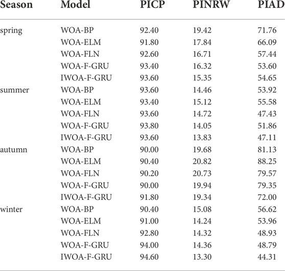
TABLE 5. Evaluation index of four network models in test dataset.

4.4 Comparison of decomposition methods

The proposed VMD-IWOA-F-GRU framework was compared with the IWOA-F-GRU, EMD-IWOA-F-GRU, and EEMD-IWOA-F-GRU at the 90% confidence level. Figure 6 shows the prediction results of the four models based on the F-GRU. The PICP, PINRW, and PIAD of the four models in the four seasons are provided in Table 6.

FIGURE 6

FIGURE 6. Prediction results of different models for four different seasons.

TABLE 6

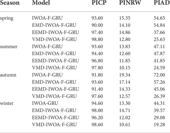
TABLE 6. Evaluation index of five prediction models in test dataset.

Figure 6 shows that the proposed model has a larger PICP value and smaller PINAW value, which proves the superiority of the proposed model for the wind power prediction. Overall, the PICP of prediction models applying the decomposition method to the original data is significantly higher than the preset confidence level. However, confounding occurs in the EMD and EEMD during the decomposition of wind power data, which increases the fitting difficulty. The number of EMD and EEMD decomposition layers reaches 13, which increases the computational cost. In contrast, the original wind power series can be decomposed well with VMD. Based on the combination of the strong generalization ability of the F-GRU and optimized objective function, the actual power values are as close to the center of the prediction interval as possible, yielding a high prediction accuracy. In conclusion, the prediction index of the VMD-IWOA-F-GRU is significantly better than that of the other four prediction models in all four seasons. Based on the above-mentioned results, the VMD-IWOA-F-GRU prediction model effectively predicts the wind power interval, with a higher accuracy and smaller bandwidth.

5 Conclusion

Due to the rapid development of wind power, wind power prediction has become the key to solve problems of wind power systems. Interval prediction is a method based on which the wind power can be effectively and quantitatively predicted. In this study, a wind power interval prediction model was established in which VMD is utilized for the decomposition of the original wind power sequence. In order to reduce the parameters to be trained and improve the training speed, F-GRU network model was proposed, and the F-GRU is employed to predict the decomposed modes. Finally, IWOA is applied to optimize the F-GRU parameters.

To verify the effectiveness of VMD-IWOA-F-GRU, the four seasons wind power datasets extracted from a wind farm was applied, and the following conclusions could be drawn according to the experimental results:

1) By comparing the F-GRU proposed in this paper and the traditional models such as BP, ELM and FLN, the F-GRU network model has better generalization ability.

2) VMD was used to decompose the wind power data, and the decomposed modes were trained independently using F-GRU and IWOA. Experiments show that the hybrid model VMD-IWOA-F-GRU proposed in this paper performs well in wind power prediction.

Data availability statement

The original contributions presented in the study are included in the article/supplementary material, further inquiries can be directed to the corresponding author.

Author contributions

DZ: Conceptualization, Methodology, Formal analysis, Investigation, Writing-Original Draft. ZZ: Methodology, Writing-Original Draft. ZC: Data Curation, Formal analysis. YZ: Writing-Review and Editing. FL: Methodology. CC: Writing-Review and Editing.

Funding

This work was supported in part by the Hainan Provincial Natural Science Foundation of China under Grants 621QN0888, and 621QN242, and in part by the Academician Workstation of Hainan Province of China Grants YSPTZX202036.

Conflict of interest

ZC was employed by the company Huaneng Clean Energy Branch.

The remaining authors declare that the research was conducted in the absence of any commercial or financial relationships that could be construed as a potential conflict of interest.

Publisher’s note

All claims expressed in this article are solely those of the authors and do not necessarily represent those of their affiliated organizations, or those of the publisher, the editors and the reviewers. Any product that may be evaluated in this article, or claim that may be made by its manufacturer, is not guaranteed or endorsed by the publisher.

References

Afshari-lgder, M., Niknam, T., and Khooban, M. H. (2018). Probabilistic wind power forecasting using a novel hybrid intelligent method. Neural comput. Appl. 30, 473–485. doi:10.1007/s00521-016-2703-z

CrossRef Full Text | Google Scholar

An, G. Q., Jiang, Z. Y., Cao, X., Liang, Y. F., Zhao, Y. Y., Li, Z., et al. (2021). Short-term wind power prediction based on particle swarm optimization-extreme learning machine model combined with adaboost algorithm. IEEE Access 9, 94040–94052. doi:10.1109/ACCESS.2021.3093646

CrossRef Full Text | Google Scholar

Bazionis, I. K., Kousounadis-Knudsen, M. A., Konstantinou, T., and Georgilakis, P. S. (2021). Wind speed forecasting method based on deep learning strategy using empirical wavelet transform, long short term memory neural network and elman neural network. Energies 14, 5942. doi:10.3390/en14185942

CrossRef Full Text | Google Scholar

Bessa, R. J., Miranda, V., Botterud, A., Zhou, Z., and Wang, J. (2012). Time-adaptive quantile-copula for wind power probabilistic forecasting. Renew. Energy 40, 29–39. doi:10.1016/j.renene.2011.08.015

CrossRef Full Text | Google Scholar

Chen, W. J., Qi, W. W., Li, Y., Zhang, J. e. a., Zhu, F., Xie, D., et al. (2021). Ultra-short-term wind power prediction based on bidirectional gated recurrent unit and transfer learning. Front. Energy Res. 9. doi:10.3389/fenrg.2021.808116

CrossRef Full Text | Google Scholar

Devi, A. S., Maragatham, G., Boopathi, K., and Rangaraj, A. G. (2020). Hourly day-ahead wind power forecasting with the eemd-cso-lstm-efg deep learning technique. Soft Comput. 24, 12391–12411. doi:10.1007/s00500-020-04680-7

CrossRef Full Text | Google Scholar

Ding, J. L., Chen, G. C., and Yuan, K. (2020). Short-term wind power prediction based on improved grey wolf optimization algorithm for extreme learning machine. Processes 8, 109. doi:10.3390/pr8010109

CrossRef Full Text | Google Scholar

Dong, Y. C., Zhang, H. L., Wang, C., and Zhou, X. J. (2021). A novel hybrid model based on bernstein polynomial with mixture of Gaussians for wind power forecasting. Appl. Energy 286, 116545. doi:10.1016/j.apenergy.2021.116545

CrossRef Full Text | Google Scholar

Dragomiretskiy, K., and Zosso, D. (2014). Variational mode decomposition. IEEE Trans. Signal Process. 62, 531–544. doi:10.1109/TSP.2013.2288675

CrossRef Full Text | Google Scholar

Duan, J. D., Wang, P., Ma, W., Fang, S., and Hou, Z. Q. (2022). A novel hybrid model based on nonlinear weighted combination for short-term wind power forecasting. Int. J. Electr. Power & Energy Syst. 134, 107452. doi:10.1016/j.ijepes.2021.107452

CrossRef Full Text | Google Scholar

Foley, A. M., Leahy, P. G., Marvuglia, A., and Mckeogh, E. J. (2012). Current methods and advances in forecasting of wind power generation. Renew. Energy 37, 1–8. doi:10.1016/j.renene.2011.05.033

CrossRef Full Text | Google Scholar

Huang, G. B., and Siew, C. K. (2004). “Extreme learning machine: Rbf network case,” in 2004 8th international conference on control, automation, robotics and vision, 1029–1036.

Google Scholar

Ji, F., Cai, X. G., and Zhang, J. H. (2015). Wind power prediction interval estimation method using wavelet-transform neuro-fuzzy network. J. Intelligent Fuzzy Syst. 29, 2439–2445. doi:10.3233/IFS-151944

CrossRef Full Text | Google Scholar

Khosravi, A., Mazloumi, E., Nahavandi, S., Creighton, D., and Van Lint, J. W. C. (2011a). Prediction intervals to account for uncertainties in travel time prediction. IEEE Trans. Intell. Transp. Syst. 12, 537–547. doi:10.1109/TITS.2011.2106209

CrossRef Full Text | Google Scholar

Khosravi, A., Nahavandi, S., Creighton, D., and Atiya, A. F. (2011b). Lower upper bound estimation method for construction of neural network-based prediction intervals. IEEE Trans. Neural Netw. 22, 337–346. doi:10.1109/TNN.2010.2096824

PubMed Abstract | CrossRef Full Text | Google Scholar

Lee, C. Y., and Zhuo, G. L. (2021). A hybrid whale optimization algorithm for global optimization. Mathematics 9, 1477. doi:10.3390/math9131477

CrossRef Full Text | Google Scholar

Li, G. Q., Niu, P. F., Duan, X. L., and Zhang, X. Y. (2016). Fast learning network: a novel artificial neural network with a fast learning speed. Neural comput. Appl. 24, 1683–1695. doi:10.1007/s00521-013-1398-7

CrossRef Full Text | Google Scholar

Li, L. L., Liu, Z. F., Tseng, M. L., Jantarakolica, K., and Lim, M. K. (2021). Using enhanced crow search algorithm optimization-extreme learning machine model to forecast short-term wind power. Expert Syst. Appl. 184, 115579. doi:10.1016/j.eswa.2021.115579

CrossRef Full Text | Google Scholar

Liu, X., Yang, L. X., and Zhang, Z. J. (2021). Short-term multi-step ahead wind power predictions based on a novel deep convolutional recurrent network method. IEEE Trans. Sustain. Energy 12, 1820–1833. doi:10.1109/TSTE.2021.3067436

CrossRef Full Text | Google Scholar

Meng, X. Y., Wang, R. H., Zhang, X. P., Wang, M. J., Qiu, G., and Wang, Z. X. (2021). Super short term wind power forecasting based on eemd-woa-lssvm. J. Comput. Appl. 41, 237–242.

Google Scholar

Mirjalili, S., and Lewis, A. (2016). The whale optimization algorithm. Adv. Eng. Softw. 95, 51–67. doi:10.1016/j.advengsoft.2016.01.008

CrossRef Full Text | Google Scholar

Naik, J., Satapathy, P., and Dash, P. K. (2018). Short-term wind speed and wind power prediction using hybrid empirical mode decomposition and kernel ridge regression. Appl. Soft Comput. 70, 1167–1188. doi:10.1016/j.asoc.2017.12.010

CrossRef Full Text | Google Scholar

Pan, J. S., Shan, J., Zheng, S. G., Chu, S. C., and Chang, C. K. (2021). Wind power prediction based on neural network with optimization of adaptive multi-group salp swarm algorithm. Clust. Comput. 24, 2083–2098. doi:10.1007/s10586-021-03247-x

CrossRef Full Text | Google Scholar

Peng, X. S., Wang, H. Y., Lang, J. X., Li, W. Z., Xu, Q., Zhang, Z., et al. (2021). Ealstm-qr: Interval wind-power prediction model based on numerical weather prediction and deep learning. Energy 220, 119692. doi:10.1016/j.energy.2020.119692

CrossRef Full Text | Google Scholar

Qiu, X. G., Wang, R. Z., Zhang, W. G., Zhang, Z. Z., and Zhang, J. (2021). Improved whale optimization algorithm based on hybrid strategy. Comput. Eng. Appl. 36, 3647–3651.

Google Scholar

Ren, F., and Long, D. H. (2021). Carbon emission forecasting and scenario analysis in guangdong province based on optimized fast learning network. J. Clean. Prod. 317, 128408. doi:10.1016/j.jclepro.2021.128408

CrossRef Full Text | Google Scholar

Saafan, M. M., and El-Gendy, E. M. (2021). Iwossa: an improved whale optimization salp swarm algorithm for solving optimization problems. Expert Syst. Appl. 176, 114901. doi:10.1016/j.eswa.2021.114901

CrossRef Full Text | Google Scholar

Sideratos, G., and Hatziargyriou, N. D. (2007). An advanced statistical method for wind power forecasting. IEEE Trans. Power Syst. 22, 258–265. doi:10.1109/TPWRS.2006.889078

CrossRef Full Text | Google Scholar

Ul Haque, A., Nehrir, M. H., and Mandal, P. (2014). A hybrid intelligent model for deterministic and quantile regression approach for probabilistic wind power forecasting. IEEE Trans. Power Syst. 29, 1663–1672. doi:10.1109/TPWRS.2014.2299801

CrossRef Full Text | Google Scholar

Wan, C., Xu, Z., Pinson, P., Dong, Z. Y., and Wong, K. P. (2014). Probabilistic forecasting of wind power generation using extreme learning machine. IEEE Trans. Power Syst. 29, 1033–1044. doi:10.1109/TPWRS.2013.2287871

CrossRef Full Text | Google Scholar

Wang, B., Li, W., Chen, X. H., and Chen, H. H. (2019). Improved chicken swarm algorithms based on chaos theory and its application in wind power interval prediction. Math. Problems Eng. 2019, 1–10. doi:10.1155/2019/1240717

CrossRef Full Text | Google Scholar

Wang, R. H., Li, C. S., Fu, W. L., and Tang, G. (2020). Deep learning method based on gated recurrent unit and variational mode decomposition for short-term wind power interval prediction. IEEE Trans. Neural Netw. Learn. Syst. 31, 3814–3827. doi:10.1109/tnnls.2019.2946414

PubMed Abstract | CrossRef Full Text | Google Scholar

Wang, H. K., Song, K., and Cheng, Y. (2022). A hybrid forecasting model based on cnn and informer for short-term wind power. Front. Energy Res. 9. doi:10.3389/fenrg.2021.788320

CrossRef Full Text | Google Scholar

Xie, L. R., Wang, B., Bao, H. Y., Liang, W. X., and Maimaitireyimu, A. (2021). Super short term wind power forecasting based on eemd-woa-lssvm. Acta Energiae Solaris Sin. 42, 290–296.

Google Scholar

Yang, X. Y., Guo, F., Zhang, Y., Kang, N., and Gao, F. (2017). A naive bayesian wind power interval prediction approach based on rough set attribute reduction and weight optimization. Energies 10, 1903. doi:10.3390/en10111903

CrossRef Full Text | Google Scholar

Yang, X. Y., Xing, G. T., Ma, X., and Fu, G. (2020a). A model of quantile regression with kernel extreme learning machine and wind power interval prediction. Acta Energiae Solaris Sin. 41, 300–306.

Google Scholar

Yang, X. Y., Zhang, Y. F., Ye, T. Z., and Su, J. (2020b). Prediction of combination probability interval of wind power based on naive bayes. High. Volt. Eng. 46, 1096–1104.

Google Scholar

Zhang, J. H., Yan, J., Infield, D., Liu, Y. Q., and Lien, F. S. (2019). Short-term forecasting and uncertainty analysis of wind turbine power based on long short-term memory network and Gaussian mixture model. Appl. Energy 241, 229–244. doi:10.1016/j.apenergy.2019.03.044

CrossRef Full Text | Google Scholar

Zhang, D. W., Chen, Z. G., and Zhou, Y. (2022a). Wind power interval prediction based on improved whale optimization algorithm and fast learning network. J. Electr. Eng. Technol. 17, 1785–1802. doi:10.1007/s42835-022-01014-5

CrossRef Full Text | Google Scholar

Zhang, S. H., Wang, C., Liao, P., Xiao, L., and Fu, T. L. (2022b). Wind speed forecasting based on model selection, fuzzy cluster, and multi-objective algorithm and wind energy simulation by betz’s theory. Expert Syst. Appl. 193, 116509. doi:10.1016/j.eswa.2022.116509

CrossRef Full Text | Google Scholar

Zhao, X. D., Fang, Y. M., Liu, L., Xu, M., and Zhang, P. (2020). Ameliorated moth-flame algorithm and its application for modeling of silicon content in liquid iron of blast furnace based fast learning network. Appl. Soft Comput. 94, 106418. doi:10.1016/j.asoc.2020.106418

CrossRef Full Text | Google Scholar