A robust flexibility evaluation method for distributed multi-energy microgrid in supporting power distribution system

Today’s power system is facing various challenges brought by large-scale renewable energy (RE) integration, which brings higher demand for flexibility. With the energy network gradually showing its distributed structural characteristics, multi-energy microgrids (MEMG) become an important component to effectively utilize distributed energy sources and supplement the flexibility of power distribution system (PDS). To effectively harness the operational flexibility of distributed MEMGs, we propose in this paper an evaluation method to quantify the flexibility capability of MEMG. A virtually established MG flexibility bus (MG-FB) is endowed with MG flexibility parameters (MG-FPs), which can reflect the flexibility characteristics of MEMG. To consider the impact of operational uncertainty on MG-FPs, a two-stage adaptive robust optimization (ARO) model is proposed, which can be solved by the C&CG algorithm. The results of a typical test system show the influence of system configuration, operator’s risk preference, and other factors on the values of MG-FPs. Besides, we illustrate the effectiveness and applicability of the proposed framework in modeling and quantifying the operational flexibility of MEMG to support the operation of the upstream network.

1 Introduction

In recent years, due to the practical need of alleviating the shortage of fossil fuels and environmental pollution, renewable energy (RE) generation forms dominated by wind power and photovoltaics have developed rapidly (Chen et al., 2016). Microgrid (MG), as an effective carrier of RE access, has been vigorously developed (Wu et al., 2021). MGs have several capital advantages, such as improving power quality, enhancing energy supply reliability, improving energy efficiency, etc. Future power grids can be pictured as systems of interconnected MGs (Parhizi et al., 2015). However, uncertainties from the RE and load-side pose some challenges to system operation. Many studies have focused on methods for forecasting RE output and load-side demand (Zang et al., 2020; Zang et al., 2021). In addition to this, increasing the operational flexibility of MGs is an unavoidable key aspect of dealing with uncertainties (Wang and Hodge, 2017; Ding et al., 2022). The application of multi-energy microgrid (MEMG) provides an important avenue to improve operational flexibility. It is inevitable to tap the flexibility potential of the MEMG system and fully plan the flexible resources in the scheduling process (Holttinen et al., 2013; Ma et al., 2013; Lund et al., 2015; Trovato et al., 2018), which implies the requirement of formulating a reasonable method to evaluate the flexibility margin of flexible resources in the MEMG system.

Flexibility can be explained as the ability of the system to cope with uncertainty. Some significant researches have been carried out, evaluating the flexibility level of power system (De Coninck and Helsen, 2016; Lu et al., 2018; Liu et al., 2021). It is proposed in (Makarov et al., 2009) the indicators for evaluating the technical operation flexibility of power system, namely power ramp-rate, power capacity, energy capacity, and ramp duration. The meaning of these indicators are further discussed in (Ulbig and Andersson, 2012). Based on these basic indicators, more research works have been conducted on evaluating the flexibility of power system. In (Lannoye et al., 2012, 2015), a probability metric called insufficient ramping resource expectation is proposed to evaluate the flexibility of the power system for use in long-term planning, which is derived from traditional generation adequacy metrics. A unified flexibility framework is proposed in (Zhao et al., 2016) to define and quantify power system flexibility in a systematic way which is based on four essential elements that are common to various applications of flexibility. In (Zhao et al., 2015), the concept of the do-not-exceed limit is introduced, which is the maximum renewable generation range that the power system can accommodate under the worst case. These studies focus on the flexibility of power system and provide basic research ideas for the flexibility evaluation of multi-energy systems.

The multi-energy coupling operation mode expands the regulation capacity of the single power system and plays a key role in emission reduction (Mancarella, 2014; Martinez Cesena et al., 2019; Wu et al., 2022). However, the complex energy conversion relationship and non-linear characteristics bring challenges to the operational flexibility evaluation. There have been several studies on the integrated operational flexibility of multi-energy systems from different perspectives. The flexible conversions of energy forms, large-scale heat and gas storage, load with different energy consumption characteristics on the demand side, etc. Are important flexibility resources in multi-energy systems. In (Wang et al., 2018), flexibility brought by energy conversion is analyzed and quantitatively evaluated based on the energy hub (EH) model. Flexibility brought by hybrid energy storage is researched in (Jiang and Hong, 2013) by assessing the benefits of smoothing out wind power fluctuations. Modeling and evaluation of flexible demand in heat and electricity integrated systems are researched in (Shao et al., 2018). A novel geometric approach is proposed in (Zhao L. et al., 2017) to characterize the aggregated flexibility of a population of thermostatically controlled loads. Besides, collaborative use of various units in multiple energy carrier operation can give play to the inherent advantages of various units’ attributes. Literature (Ulbig and Andersson, 2014) researches the flexibility of combined equipment by solving the Minkowski sum. The results show that fast frequency regulation can be provided by combining the dynamic slow power plant with the dynamic fast but energy-limited storage unit. How to obtain the most beneficial aggregated operational flexibility within a pool of different units is still the content to be studied in the future. The researches above mainly focus on the flexibility capacity of a certain component or combination benefits of some links in the system, however, the synergy of components in the multi-energy systems is neglected and the integrated flexibility of multi-energy operation is not elaborately characterized. Moreover, the transmission constraints of the networks are not taken into account.

With the large-scale access of various distributed resources such as wind power and gas turbines (GT) in recent years, load-side users have gradually transformed into MEMGs that can operate independently, and their prosumer characteristics have brought possibilities for flexibility applications in supporting PDS. In reference (Holjevac et al., 2015), the flexibility of MEMG is analyzed from two perspectives: independent of the distribution grid and in interaction with the upstream system. In reference (Capuder and Mancarella, 2014), the flexibility of coupled operation of different components in MEMG is considered. A flexibility-oriented MEMG optimization scheduling model is proposed in (Majzoobi and Khodaei, 2017) to efficiently schedule MEMG resources to meet the flexible demand of the distribution network. To address the day-ahead self-scheduling problem of the MG flexibility resources, a two-stage stochastic optimization method is developed in (Bahramara et al., 2022). However, these studies lack specific modeling and quantification of the flexibility characteristics of the MEMG. In reference (Chen and Li, 2021), the flexibility of distributed energy resources is aggregated and characterized by a parameterized set, this method can be further applied to evaluate the flexibility of MEMG. However, the significant uncertainties that affect the operational flexibility are not considered, resulting in inaccurate assessment.

To address the challenges above, we propose an evaluation method to quantify the aggregate flexibility of MEMG. We consider MEMG components of several types to fully explore the flexibility of the MEMG and the synergy between the components. Significant operational uncertainties are considered in the evaluation process, making the results robust and capable of being realized by the MEMG in its actual operation. There is data and energy interaction between MEMG and PDS, as shown in Figure 1. The quantitative MEMG flexibility capability in power exchange with the upstream network in the grid-connected mode is the focus of this paper. With the proposed method in this paper, the flexibility of the MEMG is represented by a specific set of parameters, and the power exchange efficiency between the MEMG and the PDS can be improved. In order to consider operational uncertainties in evaluating the flexible level of MEMG, the two-stage adaptive robust optimization (ARO) method is adopted. The ARO method has been widely applied to power system, such as unit commitment (Zhang et al., 2019; Dehghan et al., 2021), economic dispatch (Baringo et al., 2019; Yan et al., 2019), DER capacity assessment (Zhao J. et al., 2017; Chen et al., 2018), Resilient dispatch (Xiang and Wang, 2019; Yan et al., 2021), Active/reactive power coordination (Wu and Conejo, 2020; Huang et al., 2022), etc., mature ARO solution methods, e.g. the column-constraint-generation (C&CG) algorithm (Zeng and Zhao, 2013; Ding et al., 2017), can be directly applied as an efficient solution.

FIGURE 1

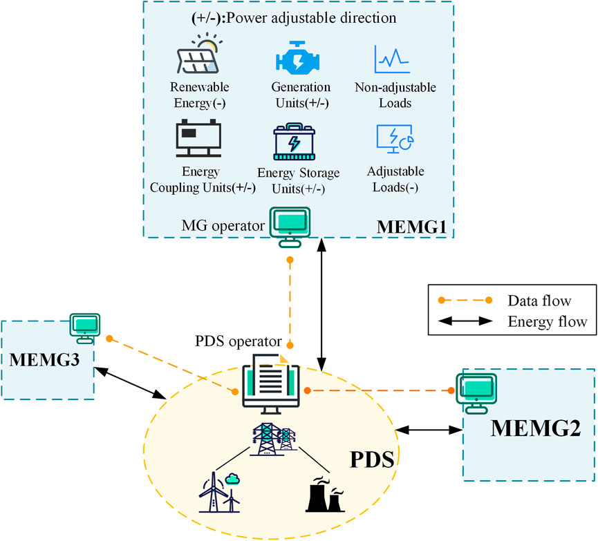
FIGURE 1. MG-PDS interactive structure.

The major contributions of this paper are threefold:

1) The flexibility-oriented model of MEMG is comprehensively proposed with consideration of energy generation-, conversion-, storage- and load-side, as well as the flexibility utility of gas and heat pipelines’ storage effect.

2) Set virtual MG-FB between MEMG and PDS and specify its properties, which are recorded as MG-FPs. The flexibility capability of MEMG is quantified by the MG-FPs which reflect the energy support effect of MEMG on PDS. This aggregated flexibility model is developed in the form of conventional generator model, which incorporates attributes of various units into simplified parameters.

3) A two-stage ARO method is developed by which the MG-FPs can be obtained. To ensure the robustness of the results, a variety of uncertainties are considered, including the uncertainty of RE power, load profiles, and dispatch instructions from the PDS. Besides, the impact of several factors on the values of MG-FPs is researched based on case study results.

The remaining part of this paper is organized as follows: Section 2 proposes the operational flexibility model and operational uncertainty set of MEMG. Section 3 presents the detailed ARO model and the C&CG algorithm for obtaining MG-FPs. Section 4 verifies the effectiveness of the proposed method for obtaining MG-FPs and researches the impact of several factors on the values of MG-FPs. Finally, Section 5 concludes the paper.

2 Operational flexibility model of MEMG

In this paper, the operational flexibility of units or systems is embodied as power and ramping rate adjustment capability, specifically, ${\mathrm{\Omega }}^{flex}:=\left\{\overline{P},\overline{P},\overline{RU},\overline{RD}\right\}$. For MEMG, a virtually established MG flexibility bus (MG-FB) is endowed with these attributes, which are denoted by MG-FPs. We define the operational flexibility region in the form of time-decoupled intervals, which is simple and efficient for model analysis and practical applications. The typical MEMG structure including various types of units and multi-energy flow is shown in Figure 2. Photovoltaic (PV) unit, wind turbine (WT), diesel generator (DG), gas turbine (GT), power to gas (P2G), electric boiler (EB), energy storage cell (ESC), gas storage tank (GST) and heat storage tank (HST) are considered in the MEMG model.

FIGURE 2

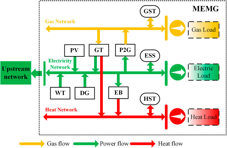
FIGURE 2. Typical MEMG structure incorporated with multiple components.

2.1 Flexibility model of MEMG components

To obtain MG-FPs, we first propose the flexibility models of the MEMG components.

2.1.1 Renewable energy unit

WT and PV units in the MEMG are considered, and the related constraints are as follows:

${\overline{P}}_i^{WT}\le p_{i,t}^{WT}\le \min \left\{{\overline{P}}_i^{WT},u_{i,t}^{WT}\right\},\forall t\in \mathit{T}(1)$

${\overline{P}}_i^{PV}\le p_{i,t}^{PV}\le \min \left\{{\overline{P}}_i^{PV},u_{i,t}^{PV}\right\},\forall t\in \mathit{T}(2)$

$v_{i,t}^{WT}=u_{i,t}^{WT}-p_{i,t}^{WT}(3)$

$v_{i,t}^{PV}=u_{i,t}^{PV}-p_{i,t}^{PV}(4)$

where $p_{i,t}^{WT}$ and $p_{i,t}^{PV}$ are output of WT i and PV unit i at time t, respectively. ${\overline{P}}_i^{WT}$, ${\overline{P}}_i^{WT}$,${\overline{P}}_i^{PV}$ and ${\overline{P}}_i^{PV}$ are output limits of WT i and PV unit i. $u_{i,t}^{WT}$ and $u_{i,t}^{PV}$ denote the available wind power and PV power of WT i and PV unit i at time t considering environmental factors. Curtailment of wind power and PV power of WT i and PV unit i at time t are denoted by $v_{i,t}^{WT}$ and $v_{i,t}^{PV}$. The output of RE units is restrained by the equipment properties and the environmental factors, as shown in Eqs.1, 2. Curtailment of RE are calculated as Eqs.3, 4.

2.1.2 Diesel generator

The operation constraints of diesel generator (DG) are as follows:

${\overline{P}}_i^{DG}{x}_{i,t}^{DG}\le p_{i,t}^{DG}\le {\overline{P}}_i^{DG}{x}_{i,t}^{DG},\forall t\in \mathit{T}(5)$

$-{\overline{RD}}_i^{DG}\le p_{i,t}^{DG}-p_{i,t-1}^{DG}\le {\overline{RU}}_i^{DG},\forall t\in \mathit{T}(6)$

$x_{i,\tau }^{DG}\ge x_{i,t}^{DG}-x_{i,t-1}^{DG},\tau =t+1,...,\min \left(t+T_i^{DG,on}-1,T^m\right),\forall t\in \mathit{T}(7)$

where $p_{i,t}^{DG}$is the output of DG i at time t, ${\overline{P}}_i^{DG}$ and ${\overline{P}}_i^{DG}$ are the minimum and maximum output of DG i, and $x_{i,t}^{DG}$ is the state variable of DG i at time t. ${\overline{RD}}_i^{DG}$ and ${\overline{RU}}_i^{DG}$ are the maximum ramp-down rate and ramp-up rate of DG i. $T_i^{DG,on}$ is the minimum on-time of DG i. $T^m$ is the time horizon of the optimization. Constraints Eqs. 5, 6 refers to the operating power constraint and ramping rate constraint of DG. Constraint Eq. 7 is the start-stop constraint of DG to avoid frequent startup and shutdown in a short time. It should be noted that the state variables are binary variables. When the state variable of DG is 1, the DG is turned on and the output power is between the maximum and minimum power output. When the state variable is 0, the DG is turned off and the power output is 0.

2.1.3 Gas turbine

The operation constraints of gas turbine (GT) are as follows:

$p_{i,t}^{GT}=g_{i,t}^{GT}{\eta }_i^{GT},\forall t\in \mathit{T}(8)$

$h_{i,t}^{GT}=p_{i,t}^{GT}{\mu }_i^{GT},\forall t\in \mathit{T}(9)$

${\overline{P}}_i^{GT}{x}_{i,t}^{GT}\le p_{i,t}^{GT}\le {\overline{P}}_i^{GT}{x}_{i.t}^{GT},\forall t\in \mathit{T}(10)$

$-{\overline{RD}}_i^{GT}\le p_{i,t}^{GT}-p_{i,t-1}^{GT}\le {\overline{RU}}_i^{GT},\forall t\in \mathit{T}(11)$

$x_{i,\tau }^{GT}\ge x_{i,t}^{GT}-x_{i,t-1}^{GT},\tau =t+1,...,\min \left(t+T_i^{GT,on}-1,T^m\right),\forall t\in \mathit{T}(12)$

where $p_{i,t}^{GT}$,$h_{i,t}^{GT}$ and $g_{i,t}^{GT}$ are electric power output, heat power output, and gas input of GT i at time t, respectively. ${\eta }_i^{GT}$denotes the power efficiency of GT i, ${\mu }_i^{GT}$is the electrothermal ratio of GT i. ${\overline{P}}_i^{GT}$and ${\overline{P}}_i^{GT}$ are the minimum and maximum output of GT i, and $x_{i,t}^{GT}$ is the state variable of GT i at time t. ${\overline{RD}}_i^{GT}$ and ${\overline{RU}}_i^{GT}$ are the maximum ramp-down rate and ramp-up rate of GT i. $T_i^{GT,on}$ is the minimum on-time of GT i. Constraints Eqs. 8, 9 depict the energy conversion relationship of GT. Constraints Eqs. 10, 11 describe the output power constraint and ramping rate constraint of GT. The operating state constraint of GT is presented in (Eq. 12).

2.1.4 Power to gas

The operation constraints of power to gas (P2G) are as follows:

$g_{i,t}^{P2G}={\delta }_i^{P2G}{p}_{i,t}^{P2G},\forall t\in \mathit{T}(13)$

${\overline{P}}_i^{P2G}{x}_{i,t}^{P2G}\le p_{i,t}^{P2G}\le {\overline{P}}_i^{P2G}{x}_{i.t}^{P2G},\forall t\in \mathit{T}(14)$

$x_{i,\tau }^{P2G}\ge x_{i,t}^{P2G}-x_{i,t-1}^{P2G},\tau =t+1,...,\min \left(t+T_i^{P2G,on}-1,T^m\right),\forall t\in \mathit{T}(15)$

where$g_{i,t}^{P2G}$ and $p_{i,t}^{P2G}$are gas output and power input of P2G i at time t, respectively. ${\delta }_i^{P2G}$is the conversion efficiency of P2G i. ${\overline{P}}_i^{P2G}$ and ${\overline{P}}_i^{P2G}$ are the minimum and maximum output of P2G i, and $x_{i.t}^{P2G}$ is the state variable of P2G i at time t. $T_i^{P2G,on}$ is the minimum on-time of P2G i. Constraint (Eq. 13) depicts the energy conversion relationship of P2G. Constraint (Eq. 14) describes the output power limit of P2G. The operating state constraint of P2G is presented in (Eq. 15).

2.1.5 Electric boiler

The constraints of the electric boiler (EB) are as follows:

$h_{i,t}^{EB}={\mu }_i^{EB}{p}_{i,t}^{EB},\forall t\in \mathit{T}(16)$

${\overline{P}}_i^{EB}{x}_{i,t}^{EB}\le p_{i,t}^{EB}\le {\overline{P}}_i^{EB}{x}_{i,t}^{EB},\forall t\in \mathit{T}(17)$

$-{\overline{RD}}_i^{EB}\le p_{i,t}^{EB}-p_{i,t-1}^{EB}\le {\overline{RU}}_i^{EB},\forall t\in \mathit{T}(18)$

$x_{i,\tau }^{EB}\ge x_{i,t}^{EB}-x_{i,t-1}^{EB},\tau =t+1,...,\min \left(t+T_i^{EB,on}-1,T^m\right),\forall t\in \mathit{T}(19)$

where $h_{i,t}^{EB}$ and $p_{i,t}^{EB}$are heat output and power input of EB i at time t, respectively. ${\mu }_i^{EB}$is the conversion efficiency of EB i. ${\overline{P}}_i^{EB}$ and ${\overline{P}}_i^{EB}$ are the minimum and maximum output of EB i, and $x_{i,t}^{EB}$ is the state variable of EB i at time t. ${\overline{RD}}_i^{EB}$ and ${\overline{RU}}_i^{EB}$ are the maximum ramp-down rate and ramp-up rate of EB i. $T_i^{EB,on}$ is the minimum on-time of EB i. Constraint (Eq. 16) depicts the energy conversion relationship of EB. Constraints (Eqs. 17, 18) describe the output power constraint and ramping rate constraint of EB. The operating state constraint of EB is presented in (Eq. 19).

2.1.6 Energy storage system

The constraints of the energy storage systems are as follows:

$x_{i,t}^{ch,\theta }+x_{i,t}^{dis,\theta }\le 1,\forall t\in \mathit{T}(20)$

$0\le e_{i,t}^{ch,\theta }\le x_{i,t}^{ch,\theta }{\overline{E}}_i^{ch,\theta },\forall t\in \mathit{T}(21)$

$0\le e_{i,t}^{dis,\theta }\le x_{i,t}^{dis,\theta }{\overline{E}}_i^{dis,\theta },\forall t\in \mathit{T}(22)$

${\underset{¯}{E}}_i^{s,\theta }\le e_{i,t}^{s,\theta }\le {\overline{E}}_i^{s,\theta },\forall t\in \mathit{T}(23)$

where $\theta =\left\{ESC,GST,HST\right\}$, denoting electricity storage cell (ESC), gas storage tank (GST) and heat storage tank (HST), respectively. $x_{i,t}^{ch,\theta }$ and $x_{i,t}^{dis,\theta }$ denote charge and discharge state of energy storage unit i at time t, respectively. $e_{i,t}^{ch,\theta }$ and $e_{i,t}^{dis,\theta }$ are charging rate and discharging rate of energy storage unit i at time t. ${\overline{E}}_i^{ch,\theta }$ and ${\overline{E}}_i^{dis,\theta }$ are maximum charging and discharging rate of energy storage unit i. $e_{i,t}^{s,\theta }$ is the current energy storage of energy storage unit i at time t. ${\underset{¯}{E}}_i^{s,\theta }$ and ${\overline{E}}_i^{s,\theta }$ are the minimum and maximum storage of energy storage unit i. Operating state of energy storage unit is constrained by (Eq 20). Constraints (Eq. 21, 21) represent the energy storage unit charging and discharging bounds, and current storage limit of energy storage unit is presented in (Eq. 23).

2.1.7 Load model

We consider four types of electric load in the flexibility model of MEMG, which are represented in (Eqs 24–(27).

1) Fixed load

$L_{i,t}^{fix,oper}=r_i^{fix}{u}_{i,t}^e,\forall t\in \mathit{T}(24)$

2) Translatable load

$L_{i,t+\tau }^{trans,oper}=r_i^{trans}{u}_{i,t}^e,\forall t\in \mathit{T}(25)$

3) Shiftable load

${\displaystyle \sum }_{t\in T}{L}_{i,t}^{sft,oper}=r_i^{sft}{u}_{i,t}^e,\forall t\in \mathit{T}(26)$

4) Interruptible load

$0\le L_{i,t}^{int,oper}\le r_i^{int}{u}_{i,t}^e,\forall t\in \mathit{T}(27)$

where $L_{i,t}^{fix,oper}$, $L_{i,t}^{trans,oper}$, $L_{i,t}^{sft,oper}$and $L_{i,t}^{int,oper}$ are fixed load, translatable load, shiftable load and interruptible load supplied at bus i at time t, respectively. $r_i^{fix}$, $r_i^{trans}$, $r_i^{sft}$ and $r_i^{int}$ are the percentage of the four types of load at node i. $u_{i,t}^e$ is the value of electric load at bus i at time t.

$r_i^{fix}+r_i^{trans}+r_i^{sft}+r_i^{int}=1,\forall i\in {\mathrm{\Omega }}^{eload}(28)$

$L_{i,t}^{e,oper}=L_{i,t}^{fix,oper}+L_{i,t}^{trans,oper}+L_{i,t}^{sft,oper}+L_{i,t}^{int,oper}(29)$

$v_{i,t}^{eload}=r_i^{int}{u}_{i,t}^e-L_{i,t}^{int,oper}(30)$

The percentage of the four types of load are constrained by (Eq. 28) and the collection of them is denoted by ${\mathit{r}}^e=\left\{r^{fix},r^{trans},r^{sft},r^{int}\right\}$. $L_{i,t}^{e,oper}$ is the load actually supplied at bus i at time t, which is constrained by (Eq. 29). The electric load that is not supplied at electric bus i at time t, denoted by $v_{i,t}^{eload}$, is calculated as (Eq. 30). Among these four types of load, 1) is non-adjustable load, b), c), and 4) belong to adjustable load.

2.2 Model of MEMG network

2.2.1 MEMG electricity network

Model of MEMG electricity network are shown as follow:

$\begin{array}{l}{p}_{i,t}^{PDS}+{\displaystyle \sum }_{u\in i}{p}_{u,t}^{DG}+{\displaystyle \sum }_{v\in i}{p}_{v,t}^{CHP}+{\displaystyle \sum }_{w\in i}{p}_{w,t}^{PV}+{\displaystyle \sum }_{m\in i}{p}_{m,t}^{WT}+{\displaystyle \sum }_{c\in i}{p}_{c,t}^{ESC}\\ =L_{i,t}^{e,equ}+{\displaystyle \sum }_{j\in i}{p}_{ij,t}-{\displaystyle \sum }_{j\in i}{p}_{ji,t},\forall t\in \mathit{T}\end{array}(31)$

${\overline{P}}_k\le p_{k,t}\le {\overline{P}}_k,\forall t\in \mathit{T}(32)$

where $p_{i,t}^{PDS}$ denotes the power from PDS at electric bus i at time t. $p_{u,t}^{DG}$/$p_{v,t}^{CHP}$/$p_{w,t}^{PV}$/$p_{m,t}^{WT}$/$p_{c,t}^{ESC}$ is the power output of DG/CHP/PV/WT/ESC at electric bus i at time t. $L_{i,t}^{e,equ}$ denotes the equivalent electric load at electric bus i at time t. $p_{ij,t}$ is electric flow of the lines which start with electric bus i and $p_{ji,t}$ is electric flow of the lines which end with electric bus i. $p_{k,t}$denotes the electric flow of line k at time t. ${\overline{P}}_k$ and ${\overline{P}}_k$ are limits of the electric flow of line k. MEMG electricity network constraints include nodal power balance constraint (Eq. 31) and electric power line transmission capacity constraint (Eq. 32).

2.2.2 MEMG gas network

We adopt Weymouth steady-state model in this paper:

${\displaystyle \sum }_{s\in i}{g}_{s,t}^{GS}+{\displaystyle \sum }_{n\in i}{g}_{n,t}^{P2G}+{\displaystyle \sum }_{z\in i}{g}_{z,t}^{GST}=L_{i,t}^{g,equ}+{\displaystyle \sum }_{j\in i}{g}_{ij,t}-{\displaystyle \sum }_{j\in i}{g}_{ji,t},\forall t\in \mathit{T}(33)$

$V_{k,t}\left|V_{k,t}\right|=C_k\mathit{\Delta }\mathit{pr}{e}_{k,t},\forall t\in \mathit{T}(34)$

${\underset{¯}{V}}_k\le V_{k,t}\le {\overline{V}}_k,\forall t\in \mathit{T}(35)$

${\underset{¯}{pre}}_i\le \mathit{pr}{e}_{i,t}\le {\overline{pre}}_i,\forall t\in \mathit{T}(36)$

where $g_{s,t}^{GS}$/$g_{n,t}^{P2G}$/$g_{z,t}^{GST}$ is the gas output of gas source/P2G/GST at gas bus i at time t. $L_{i,t}^{g,equ}$ denotes the equivalent gas load at gas bus i at time t. $g_{ij,t}$ is gas flow of the pipelines which start with gas bus i at time t and $g_{ji,t}$is gas flow of the pipelines which end with gas bus i at time t. $V_{k,t}$ denotes the gas flow of pipeline k at time t. $C_k$ is the flow-pressure correlation coefficient. $\Delta \mathit{pr}{e}_{k,t}$ is the pressure difference between the start and the end of pipeline k. ${\underset{¯}{V}}_k$ and ${\overline{V}}_k$ are the minimum and maximum gas flow of pipeline k. $\mathit{pr}{e}_{i,t}$ is the pressure at gas bus i at time t. ${\underset{¯}{pre}}_i$ and ${\overline{pre}}_i$ are minimum and maximum pressure at gas bus i. The nodal gas balance constraint is presented in (Eq. 33). The relationship between the gas flow and nodal pressure is shown in (Eq. 34). Constraint (Eqs. 35, 36) depict the gas flow limit and nodal pressure limit, respectively. It should be noted that constraint (34) is nonlinear, and it is piecewise linearized in the following optimization model for efficient solution.

The transmission rate of gas is slow, and the gas has inertia and compressibility, so the gas transmission pipeline has a certain storage capacity. This energy storage effect can alleviate the time and space mismatch between the natural gas supply and the gas load consumption demand to a certain extent. The more natural gas stored in the pipeline, the greater the pressure at both ends of the pipeline, which are constrained by (Eq. 36).

2.2.3 MEMG heating network

We use the steady-state model of the heat supply network in this paper:

${\displaystyle \sum }_{k\in {\mathrm{\Omega }}_{sp,i-}}{T}_{k,t}^{sp,out}\cdot q_k^{sp}=T_{i,t}^{sn}{\displaystyle \sum }_{k\in {\mathrm{\Omega }}_{sp,i-}}{q}_k^{sp},\forall t\in \mathit{T}(37)$

${\displaystyle \sum }_{k\in {\mathrm{\Omega }}_{rp,i-}}{T}_{k,t}^{rp,out}\cdot q_k^{rp}=T_{i,t}^{rn}{\displaystyle \sum }_{k\in {\mathrm{\Omega }}_{rp,i-}}{q}_k^{rp},\forall t\in \mathit{T}(38)$

$T_{k,t}^{sp,in}=T_{i,t}^{sn},\forall k\in {\mathrm{\Omega }}_{sp,i+},\forall t\in \mathit{T}(39)$

$T_{k,t}^{rp,in}=T_{i,t}^{rn},\forall k\in {\mathrm{\Omega }}_{rp,i+},\forall t\in \mathit{T}(40)$

$T_{k,t}^{sp,out}=\left(T_{k,t}^{sp,in}-T_a\right)e^{-\frac{l_k}{Rc\rho f_k}}+T_{k,t}^{sp,in},\forall k\in {\mathrm{\Omega }}_{sp},\forall t\in \mathit{T}(41)$

$T_{k,t}^{rp,out}=\left(T_{k,t}^{rp,in}-T_a\right)e^{-\frac{l_k}{Rc\rho f_k}}+T_{k,t}^{rp,in},\forall k\in {\mathrm{\Omega }}_{rp},\forall t\in \mathit{T}(42)$

$T_{k,t}^{sp,out}=\left(T_a-T_{k,t}^{sp,in}\right)\frac{l_k}{Rc\rho f_k}+T_{k,t}^{sp,in},\forall k\in {\mathrm{\Omega }}_{sp},\forall t\in \mathit{T}(43)$

$T_{k,t}^{rp,out}=\left(T_a-T_{k,t}^{rp,in}\right)\frac{l_k}{Rc\rho f_k}+T_{k,t}^{rp,in},\forall k\in {\mathrm{\Omega }}_{rp},\forall t\in \mathit{T}(44)$

${\underset{¯}{T}}^{sp}\le T_{k,t}^{sp,in}\le {\overline{T}}^{sp},\forall k\in {\mathrm{\Omega }}_{sp},\forall t\in \mathit{T}(45)$

${\underset{¯}{T}}^{sp}\le T_{k,t}^{sp,out}\le {\overline{T}}^{sp},\forall k\in {\mathrm{\Omega }}_{sp},\forall t\in \mathit{T}(46)$

${\underset{¯}{T}}^{rp}\le T_{k,t}^{rp,in}\le {\overline{T}}^{rp},\forall k\in {\mathrm{\Omega }}_{rp},\forall t\in \mathit{T}(47)$

${\underset{¯}{T}}^{rp}\le T_{k,t}^{rp,out}\le {\overline{T}}^{rp},\forall k\in {\mathrm{\Omega }}_{rp},\forall t\in \mathit{T}(48)$

${\displaystyle \sum }_{k\in {\mathrm{\Omega }}_{sp,i-}}\left(C^h{q}_k^{sp}\left(T_{k,t}^{sp,out}-T_{k,t}^{rp,in}\right)\right)=L_{i,t}^{h,equ},\forall t\in \mathit{T}(49)$

where ${\mathrm{\Omega }}_{sp,i-}$ and ${\mathrm{\Omega }}_{rp,i-}$ represent the collection of water supply and return pipelines whose end point is heat bus i. ${\mathrm{\Omega }}_{sp,i+}$ and ${\mathrm{\Omega }}_{rp,i+}$ represent the collection of water supply and return pipelines whose end point is heat bus i. ${\mathrm{\Omega }}_{sp}$ and ${\mathrm{\Omega }}_{rp}$ represent the collection of water supply and return pipelines. $T_{k,t}^{sp,out}$ and $T_{k,t}^{rp,out}$ represent the temperature at the outlet of pipeline k in the water supply and return network at time t, respectively. $q_k^{sp}$ and $q_k^{rp}$ indicate the water outflowing from pipeline k in the water supply and return network, respectively. $T_{i,t}^{sn}$ and $T_{i,t}^{rn}$ are the temperature at node i within the water supply and return network at time t. $T_{k,t}^{sp,in}$ and $T_{k,t}^{rp,in}$ are the temperature at the inlet of the pipeline k in the supply and return network, respectively. The flow of heat medium in the pipeline will produce heat loss, which is related to ambient temperature $T_a$, pipeline length $l_k$, pipeline thermal resistance $R$, pipeline flow $f_k$, the specific heat capacity $c$of heat medium, and heat medium density $\rho$. ${\underset{¯}{T}}^{sp}$, ${\overline{T}}^{sp}$, ${\underset{¯}{T}}^{rp}$ and ${\overline{T}}^{rp}$are the temperature limits of water supply and return pipelines. $C^h$ is the heat capacity of the water within the pipelines. $L_{i,t}^{h,equ}$ denotes the equivalent heat load at heat bus i at time t. Eqs. 37, 38 are the node temperature fusion constraint, which indicates that the node temperature is equal to the fusion temperature of the incoming heat medium. The temperature of the heat medium flowing out of the node is equal to the temperature of the node, as depicted in constraints (Eqs. 39, 40). The temperature relationship of the heat medium at the inlet and outlet of the pipelines is shown in constraints (Eqs. 41, 42). Considering that the exponential term is close to zero, its linearized form can be obtained by Taylor expansion and omitting the higher order terms, as shown in constraints (Eqs. 43, 44). Constraints (Eqs. 45–48) are the temperature limits of the heat supply and return pipelines. Heat balance constraint of heat load node is shown as (Eq. 49).

Since the temperature of the heat pipelines can fluctuate within a certain range, as shown in (Eqs. 45–(48), the heat pipelines have a certain heat storage capacity. Heat pipelines in MEMG are flexible resources with flexible capability that can be dispatched.

2.2.4 Coupling constraints of MEMG

The coupling constraints of different networks in MEMG are as follows:

$L_{i,t}^{e,equ}=L_{i,t}^{e,oper}+{\displaystyle \sum }_{k\in {\mathrm{\Omega }}_{ECU}^i}{p}_{k,t},\forall t\in \mathit{T}(50)$

$L_{i,t}^{g,equ}=u_{i,t}^g+{\displaystyle \sum }_{k\in {\mathrm{\Omega }}_{GCU}^i}{g}_{k,t},\forall t\in \mathit{T}(51)$

$L_{i,t}^{h,equ}=u_{i,t}^h,\forall t\in \mathit{T}(52)$

where ${\mathrm{\Omega }}_{ECU}^i$/${\mathrm{\Omega }}_{GCU}^i$ is collection of power consuming units/gas consuming units at bus i, $p_{k,t}$/$g_{k,t}$ is the power consumption/gas consumption of unit k at time t. $u_{i,t}^g$ and $u_{i,t}^h$ are the value of gas load and heat load at bus i at time t. In the MEMG, in addition to the conventional user-side load, the input of the multi-energy coupling equipment is also considered as the load of the corresponding energy system. Therefore, the equivalent electric load and the equivalent gas load at node i at time t are expressed as (Eqs. 50, 51). The equivalent heat load at node i at time t is shown as (Eq. 52).

2.3 Operational uncertainty set of MEMG

MEMGs face many uncertainties in their operation and it is risky to reduce these uncertainties to predicted values. To consider these uncertain factors in evaluating the flexibility of MEMG, an ARO problem is proposed. In the ARO problem, it is important to construct a suitable uncertainty set. The uncertainty model of MEMG operation is given in this section.

2.3.1 RE output and load consumption

A way to capture RE output and load consumption uncertainty is as follows:

$\begin{array}{l}{\mathit{u}}^{RE}=\{u^{WT},u^{PV}|u_{i,t}^{WT}={\widehat{u}}_{i,t}^{WT}+{\varsigma }_i^{WT}{d}_i^{WT},{\varsigma }_i^{WT}\in \left[\mathrm{0,1}\right],d_i^{WT}/{\widehat{u}}_{i,t}^{WT}\le {\rho }^{WT},\\ u_{i,t}^{PV}={\widehat{u}}_{i,t}^{PV}+{\varsigma }_i^{PV}{d}_i^{PV},{\varsigma }_i^{PV}\in \left[\mathrm{0,1}\right],d_i^{PV}/{\widehat{u}}_{i,t}^{PV}\le {\rho }^{PV},\forall t\in \mathit{T}\}\end{array}(53)$

${\mathit{u}}^{load}=\left\{u^{\omega }|u_{j,t}^{\omega }={\widehat{u}}_{j,t}^{\omega }+{\varsigma }_j^{\omega }{d}_j^{\omega },{\varsigma }_j^{\omega }\in \left[\mathrm{0,1}\right],d_j^{\omega }/{\widehat{u}}_{j,t}^{\omega }\le {\rho }^{\omega },\omega =\left\{e,g,h\right\}\right\}(54)$

where ${\widehat{u}}_{i,t}^{WT}$ and ${\widehat{u}}_{i,t}^{PV}$ respectively represent the predicted available power of WT and PV at node i at time t. $\omega$ is a collection of energy forms in the MEMG system, including the energy form of electricity, gas and heat. ${\widehat{u}}_{j,t}^e$, ${\widehat{u}}_{j,t}^g$ and ${\widehat{u}}_{j,t}^h$ represent the predicted electric, gas and heat load consumption at load node j at time t, respectively. These predicted values are obtained based on historical data. We use the product of the maximum deviation $d_i^{WT}$/$d_i^{PV}$/$d_j^{L,\omega }$ and the error coefficient ${\varsigma }_i^{WT}$/${\varsigma }_i^{PV}$/${\varsigma }_j^{\omega }$ to express the prediction deviation of WT output/PV output/load consumption. ${\rho }^{WT}$, ${\rho }^{PV}$and ${\rho }^{\omega }$are given constants, which are introduced to define the limit of uncertainty to control the conservative level.

2.3.2 Dispatch instructions from PDS operator with carbon emission target

The uncertainty set of the dispatch instructions from the PDS operator is modeled as follows:

${\mathit{u}}^{DI}\supset \left\{P_t^{DI},R{R}_t^{DI}|{\overline{P}}^{MG}\le P_t^{DI}\le {\overline{P}}^{MG},-{\overline{RD}}^{MG}\le R{R}_t^{DI}\le {\overline{RU}}^{MG},R{R}_t^{DI}=P_{t+1}^{DI}-P_t^{DI},\forall t\in \mathit{T}\right\}(55)$

where $P_t^{DI}$ and $R{R}_t^{DI}$ are instructed power output and ramping rate at time t from the PDS. When MEMG is providing flexibility to PDS, the interaction power between MEMG and PDS is constrained by (Eqs.56, 57).

$p_t^{PDS}=P_t^{DI},\forall t\in \mathit{T}(56)$

$r_t^{PDS}=p_t^{PDS}-p_{t-1}^{PDS}=R{R}_t^{DI},\forall t\in \mathit{T}(57)$

where $p_t^{PDS}$ and $r_t^{PDS}$ are power output and ramping rate of MEMG at the MG-FB at time t.

Besides, based on the carbon reduction trend of the energy system, we add the carbon emission limits that need to be realized by MEMG to the uncertainty set of the model: ${\mathit{u}}^{DI}=\left\{P_t^{DI},R{R}_t^{DI},C{E}_t^{DI}\right\}$. Thus, the energy supply units in the MEMG can be more preferably configured based on the environmental protection objectives. The relevant constraints are shown below.

$C{E}_{m,t}={\psi }_m{p}_{m,t},\forall m\in {\mathrm{\Omega }}_{emi}(58)$

$C{E}_t={\displaystyle \sum }_{m\in {\mathrm{\Omega }}_{emi}}C{E}_{m,t}(59)$

$C{E}_t\le C{E}_t^{DI}(60)$

${\displaystyle \sum }_{t\in T}C{E}_t^{DI}\le \Gamma (61)$

${\underset{¯}{CE}}^{DI}\le C{E}_t^{DI}\le {\overline{CE}}^{DI}(62)$

where ${\mathrm{\Omega }}_{emi}$ is the collection of units with carbon emission in the MEMG. $C{E}_{m,t}$ and $p_{m,t}$ are the carbon emission and energy output of unit m at time t, respectively. ${\psi }_m$ is the carbon emission factor of unit m. $C{E}_t$ denotes the carbon emission of MEMG at time t. $C{E}_t^{DI}$ is the carbon emission limit for MEMG at time t in dispatch instructions from the PDS. $\Gamma$, ${\underset{¯}{CE}}^{DI}$ and ${\overline{CE}}^{DI}$ are pre-given constants. Part of the units in the MEMG produce pollution when operating, and the carbon emission of the units is usually proportional to the production, i.e. constraint (Eq. 58). The carbon emission of the MEMG system is the total emission of all carbon emission generating units in the system, i.e. constraint (Eq. 59). To achieve an overall carbon emission reduction target, the PDS operator will add the carbon emission constraint (Eq. 60) to MEMG in the dispatch instructions, in which the boundary is shown as (Eqs. 61, 62), which ensures that the carbon emission range of the MEMG is always kept within a reasonable range.

Based on the discussion above, operational uncertainty set of MEMG is denoted by (Eq. 63).

$\mathit{u}=\left\{{\mathit{u}}^{RE},{\mathit{u}}^{load},{\mathit{u}}^{DI}\right\}(63)$

3 ARO model for obtaining MG-FPs

3.1 ARO model

When considering the operational uncertainty, the acquisition of MG-FPs has the following steps. In step 1, the MEMG operator collects the operation parameters of various local units, and in step 2, solves the initial MG-FPs according to the MEMG flexibility model and network operation constraints. In step 3, the MEMG operator searches for possible dispatch instructions from PDS and possible operation scenarios. In step 4, the MEMG operator tries to track the dispatch instructions from PDS in different operation scenarios, and judges if these orders are realizable and whether the MG-FPs need to be adjusted. If an unrealizable scenario is found, the MEMG operator adjusts the MG-FPs in step 5. Repeat steps three to five until no infeasible scenario is found, and the MEMG operator submits the MG-FPs obtained in the latest iteration to the PDS operator.

Based on the steps above, we propose a two-stage ARO model to obtain the MG-FPs submitted by the MEMG to PDS. The upper stage problem is solved first to obtain the MG-FPs. The upper stage problem aims to maximize the MEMG’s flexibility region, including the feasible range of power, and upward and downward ramping rate. Subsequently, the lower stage problem aims to identify the worst-case uncertainty vector that maximizes the power imbalance at the MG-FB and optimizes the post-contingency dispatch with the values of MG-FPs. The convergence speed of the ARO model is accelerated by adding the worst scenario set to the upper stage problem. In the iteration process, the scenarios that are difficult to realize in the MEMG are gradually discovered, and the obtained MEMG’s flexibility domain is gradually shrinking. When no solution-free scenario can be found, the MEMG operator obtains the accurate MG-FPs.

By solving this robust problem, the obtained optimal MG-FPs results can immunize to any uncertainty within a reasonable range. When the uncertainty u* happens, the deviation caused by u* is tried to be accommodated by the MEMG post-contingency dispatch. The compact formulation of the proposed model is presented in (Eqs. 64–(70):

$\underset{\mathit{z}}{\min }\left\{-{\mathit{c}}^T\mathit{z}+\underset{\mathit{u}}{\max }\underset{\mathit{x},\mathit{y}\in \mathrm{\Omega }\left(\mathit{z},\mathit{u}\right)}{\min }{\mathit{d}}^T\mathit{y}\right\}(64)$

$s.t.\mathit{A}\mathit{x}\le \mathit{b}(65)$

$\mathit{D}\mathit{y}\le \mathit{a}(66)$

$\mathit{C}\mathit{y}+\mathit{E}\mathit{x}+\mathit{F}\mathit{u}+\mathit{G}\mathit{z}\le \mathit{h}(67)$

$\mathrm{\Omega }\left(\mathit{z},\mathit{u}\right)=\left\{\mathit{x},\mathit{y}|\mathit{C}\mathit{y}+\mathit{E}\mathit{x}\le \mathit{h}-\mathit{F}\mathit{u}-\mathit{G}\mathit{z}\right\}(68)$

$c^T\mathit{z}={\kappa }_1{\overline{P}}^{MG}+{\kappa }_2{\overline{P}}^{MG}+{\lambda }_1{\overline{RU}}^{MG}+{\lambda }_2{\overline{RD}}^{MG}(69)$

${\kappa }_1>0,{\kappa }_2<0,{\lambda }_1>0,{\lambda }_2<0(70)$

$\begin{array}{l}\mathrm{w}\mathrm{h}\mathrm{e}\mathrm{r}\mathrm{e}\mathit{x}=\{x_t^{DG},x_t^{GT},x_t^{P2G},x_t^{EB},x_t^{ch,ESC},x_t^{dis,ESC},x_t^{ch,GST},x_t^{dis,GST},x_t^{ch,HST},x_t^{dis,HST},\forall t\in \mathit{T}\},\mathit{y}=\{p_t^{WT},\\ p_t^{PV},v_t^{WT},v_t^{PV},p_t^{DG},g_t^{GT},p_t^{GT},h_t^{GT},g_t^{P2G},p_t^{P2G},h_t^{EB},p_t^{EB},e_t^{ch,\theta },e_t^{dis,\theta },e_t^{s,\theta },L_t^{fix,oper},L_t^{trans,oper},L_t^{sft,oper},L_t^{int,oper},\\ L_t^{e,oper},V_t,\mathit{\Delta }\mathit{pr}{e}_t,T_t^{sp,in},T_t^{sp,out},T_t^{sn},T_t^{rn},T_t^{rp,in},T_t^{rp,out},L_t^{e,equ},L_t^{g,equ},L_t^{h,equ},t\in \mathit{T}\},\mathit{u}=\{u_t^{WT},u_t^{PV},u_t^e,{\mathit{r}}^e,u_t^g,u_t^h,\\ P_t^{DI},R{R}_t^{DI},C{E}_t^{DI},\forall t\in \mathit{T}\}\end{array}$

Constraint 65) refers to (7), (12), (15), (19), (20). Constraint 66) represents (6), (8)–(9), (11), (13), (16), (18), (23), (29), (31)–(50), (58)–(59). Constraint 67) denotes the constraints (1)–(5), (10), (14), (17), (21)–(22), (24)–(28), (30), (51)–(57), (60)–(62).

Weight coefficients ${\kappa }_1$, ${\kappa }_2$, ${\lambda }_1$, and ${\lambda }_2$ in constraint 69) are given in advance by the MEMG operators, which could reflect their decision preferences. When ${\kappa }_1$ ($\left|{\kappa }_2\right|$) is large, a higher power upper limit (lower power inferior limit) will be obtained, but it will lead to contraction of the ramping rate adjustable range. When ${\lambda }_1$ ($\left|{\lambda }_2\right|$) is large, MEMG will have a better upward (downward) ramping rate adjustment ability, but the power adjustment ability will become worse. By selecting the weight coefficients, MEMG operator finally obtains MG-FPs of different operational flexibility characteristics. For PDS, MEMGs with different MG-FPs are equivalent to different types of generation units or loads.

3.1.1 Master problem

The primal problem can be decoupled into a master problem (MP) and a subproblem (SP). The MP is presented in (Eqs. 71–(76), which optimizes the decision variables of MG-FPs.

$MP:$

$\underset{\mathit{z}}{\min }\left(-{\mathit{c}}^T\mathit{z}\right)(71)$

$s.t.\mathit{A}\mathit{x}\le \mathit{b}(72)$

$\mathit{D}\mathit{y}\le \mathit{a}(73)$

$\mathit{C}\mathit{y}+\mathit{E}\mathit{x}+\mathit{G}\mathit{z}\le \mathit{h}-{\mathit{F}\mathit{u}}_{l-1}^{\ast },\forall l\le k(74)$

$c^T\mathit{z}={\kappa }_1{\overline{P}}^{MG}+{\kappa }_2{\overline{P}}^{MG}+{\lambda }_1{\overline{RU}}^{MG}+{\lambda }_2{\overline{RD}}^{MG}(75)$

${\kappa }_1>0,{\kappa }_2<0,{\lambda }_1>0,{\lambda }_2<0(76)$

where k denotes the current iteration. ${\mathit{u}}_{l-1}^{\ast }$is identified by the SP in the previous iteration. The optimal result of the MP is recorded as z∗, and is passed to the SP as known parameters.

3.1.2 Max-min subproblem

The SP identifies the most damaging uncertainty set for the determined MG-FPs obtained by the MP. The unsolvable scenarios are iteratively generated and added by solving the feasibility check SP. The compact form of the feasibility check SP in the kth iteration is formulated as (Eqs. 77–82). We reformulate the SP as an equivalent maximization problem (Eqs. 83–(86) using the duality principle for the initial bi-level model cannot be solved directly.

$SP:$

$\underset{\mathit{u}}{\max }\underset{\mathit{x},\mathit{y}\in \mathrm{\Omega }\left(\mathit{z},\mathit{u}\right)}{\min }{\mathit{d}}^T\mathit{y}(77)$

$s.t.\mathit{C}\mathit{y}+\mathit{E}\mathit{x}+\mathit{F}\mathit{u}\le \mathit{h}-\mathit{G}{\mathit{z}}_k^{\ast }:\left(\lambda \right)(78)$

${\mathit{d}}^T\mathit{y}=e_1{\displaystyle \sum }_{t\in T}\left({\chi }^{+}+{\chi }^{-}\right)+e_2{\displaystyle \sum }_{t\in T}\left({\delta }^{+}+{\delta }^{-}\right)(79)$

$P_t^{DI}=p_t^{PDS}+{\chi }^{+}-{\chi }^{-}(80)$

$R{R}_t^{DI}=r_t^{PDS}+{\delta }^{+}-{\delta }^{-}(81)$

${\chi }^{+}\ge 0,{\chi }^{-}\ge 0,{\delta }^{+}\ge 0,{\delta }^{-}\ge 0(82)$

$\underset{\mathit{u},\mathit{\lambda }}{\max }{\lambda }^T\left(\mathit{h}-\mathit{G}{\mathit{z}}_k^{\ast }-\mathit{F}\mathit{u}\right)(83)$

$s.t.{\mathit{\lambda }}^{T}C\le d(84)$

${\mathit{\lambda }}^{T}E\le 0(85)$

$\mathit{\lambda }\le 0(86)$

where $\lambda$ is the dual variable vector of the MEMG dispatch problem in the inner level of SP. ${\chi }^{+}$ and ${\chi }^{-}$ denote the deviation between actual power output $p_t^{PDS}$ and the instructed $P_t^{DI}$ at time t, ${\delta }^{+}$ and ${\delta }^{-}$ denotes the deviation between actual ramping rate $r_t^{PDS}$ and the instructed $R{R}_t^{DI}$. These deviations will be eliminated in the iteration procedure to ensure that the MEMG can track these dispatch instructions from the PDS operator.

3.2 The detailed solution procedure of C&CG

The proposed MP and the max-min SP are both MILP models, which can be solved by several solvers. The two-stage ARO model is solved by the C&CG Algorithm 1, which is a cutting-plane-based method. The procedure is conducted iteratively, as shown in Figure 3. Detailed steps are shown as follows.

FIGURE 3

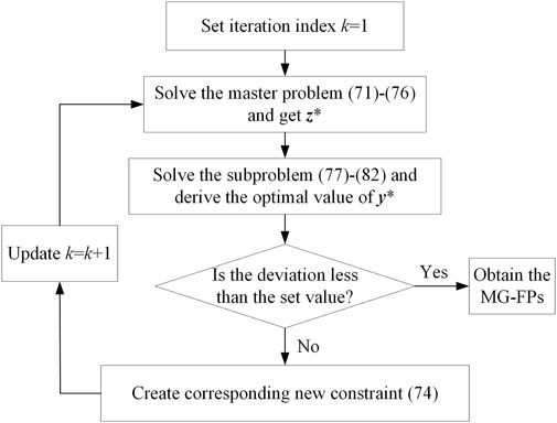
FIGURE 3. Solving procedures of C&CG algorithm.

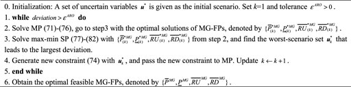
Algorithm 1. Column-and-Constraint Generation Algorithm.

4 Case study

The following cases are performed on a modified network that operates as a MEMG. Characteristics of the initial network are available in (Yang et al., 2020). The MEMG is connected to PDS for data and energy exchange. The MEMG includes 70 buses, 65 lines, and 32 loads. Besides, there are 2 DGs, 2 GTs, 2 P2G, 3 EBs, 1 PV, 1 WT, 1 ESC, 1 GST, and 1 HST. The main parameters of the units are shown in Tables 1, 2. Daily load, wind power and PV power are depicted in Figures 4, 5.

TABLE 1

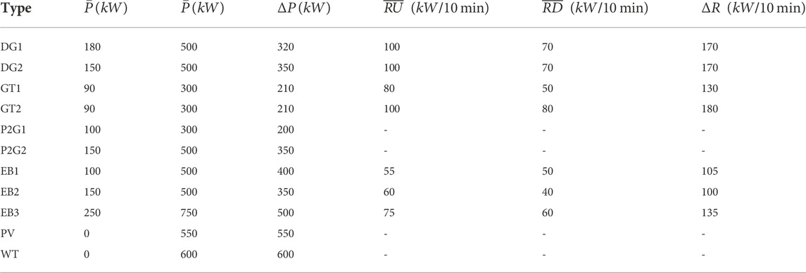
TABLE 1. Main parameters of units in MEMG.

TABLE 2

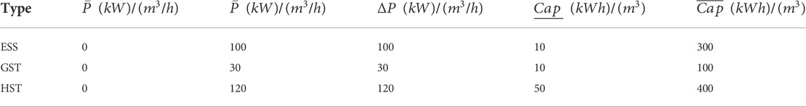
TABLE 2. Main parameters of energy storage units in MEMG.

FIGURE 4

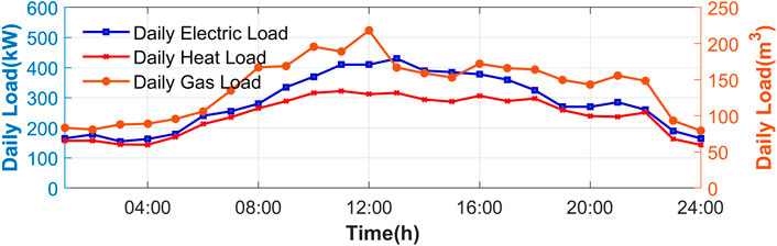
FIGURE 4. Daily load profiles of MEMG.

FIGURE 5

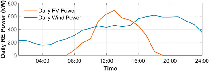
FIGURE 5. Daily RE power of MEMG.

All tests are implemented on a computer with eight processors running at 3.60 GHz with 16 GB of memory. Programs are coded under MATLAB 2019b environment and programmed with YALMIP by calling cplex.

4.1 Comparison of MG-FPs’ calculation methods

We first verify the effectiveness and accuracy of the proposed ARO model in obtaining MG-FPs. In addition to the proposed ARO method, we calculate the MG-FPs in a direct way for comparison. Table 3 shows the results of the optimized MG-FPs with the two methods. The basic equations of the direct method are as follows:

${\overline{P}}^{MG}={\displaystyle \sum }_{k\in {\mathrm{\Omega }}_{sup}}{\overline{P}}_k+{\displaystyle \sum }_{r\in {\mathrm{\Omega }}_{co}}\Delta {\overline{P}}_r-{\displaystyle \sum }_{i\in {\mathrm{\Omega }}_{EL}}{L}_i(87)$

${\overline{P}}^{MG}={\displaystyle \sum }_{k\in {\mathrm{\Omega }}_{sup}}{\overline{P}}_k+{\displaystyle \sum }_{r\in {\mathrm{\Omega }}_{co}}\Delta {\overline{P}}_r-{\displaystyle \sum }_{i\in {\mathrm{\Omega }}_{EL}}{L}_i(88)$

${\overline{RU}}^{MG}={\displaystyle \sum }_{k\in {\mathrm{\Omega }}_r}{\overline{RU}}_k(89)$

${\overline{RD}}^{MG}={\displaystyle \sum }_{k\in {\mathrm{\Omega }}_r}{\overline{RD}}_k(90)$

where${\displaystyle \sum }_{k\in {\mathrm{\Omega }}_{sup}}{\overline{P}}_k$ and${\displaystyle \sum }_{k\in {\mathrm{\Omega }}_{sup}}{\overline{P}}_k$ denote the sum of maximum and minimum output of power supply units, ${\displaystyle \sum }_{r\in {\mathrm{\Omega }}_{co}}\Delta {\overline{P}}_r$ and ${\displaystyle \sum }_{r\in {\mathrm{\Omega }}_{co}}\Delta {\overline{P}}_r$ denote the sum of maximum and minimum power output of the energy coupling units while loads of other energy types meet their demand. ${\displaystyle \sum }_{i\in {\mathrm{\Omega }}_{EL}}{L}_i$denotes the sum of electric load. ${\displaystyle \sum }_{k\in {\mathrm{\Omega }}_r}{\overline{RU}}_k$ and ${\displaystyle \sum }_{k\in {\mathrm{\Omega }}_r}{\overline{RD}}_k$ represent the sum of the maximum ramp-up rate and ramp-down rate of units in MEMG.

TABLE 3

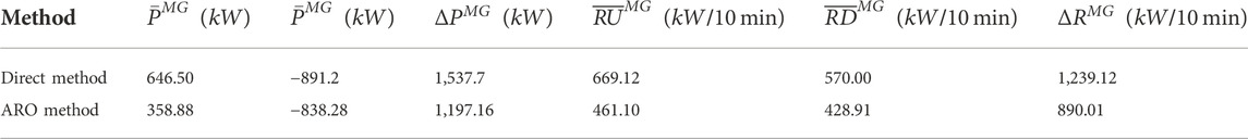
TABLE 3. Results of MG-FPs from different methods.

It is obvious that the MG-FPs obtained from the direct method have better flexibility benefits than the ARO method. But actually, these look-better parameters are hard to track for MEMGs because the direct method calculates the MG-FPs without consideration of line capacity limitation. In other words, the inaccuracy of the direct method comes mainly from the violation of network constraints when directly summing up the flexibility parameters of units. There is a possibility that the MEMG operator cannot realize the committed parameters in some scenarios without security violation.

When the power of the MEMG is negative, the PDS supplies electric power to the MEMG, MEMG is equivalent to the load of the PDS. This minimum power flexibility parameter is constrained by MEMG’s energy consumption level and energy transmission capacity. The higher the MEMG energy consumption level and the greater the line transmission capacity, the greater the absolute value of the minimum power flexibility parameter, and vice versa. When the interaction power is positive, the MEMG supplies energy to the PDS on the basis of meeting its own load demand. The maximum power flexibility parameter is limited by the energy supply capacity of energy supply equipment, conversion capacity of energy conversion equipment, and energy transmission capacity of MEMG.

4.2 Impact of MEMG Operator’s risk preference and system configuration

Adopting the robust optimization framework proposed in this paper, we can change the MEMG operator’s risk preference by changing the uncertainty parameters (UP). The UPs refer to ${\rho }^{PV}$, ${\rho }^{WT}$ and ${\rho }^{\omega }$ in the MEMG operational uncertainty model. The deterministic optimization (DO), in which the uncertainty variables take the predicted values, is also solved for comparison. The results are listed in Table 4.

TABLE 4

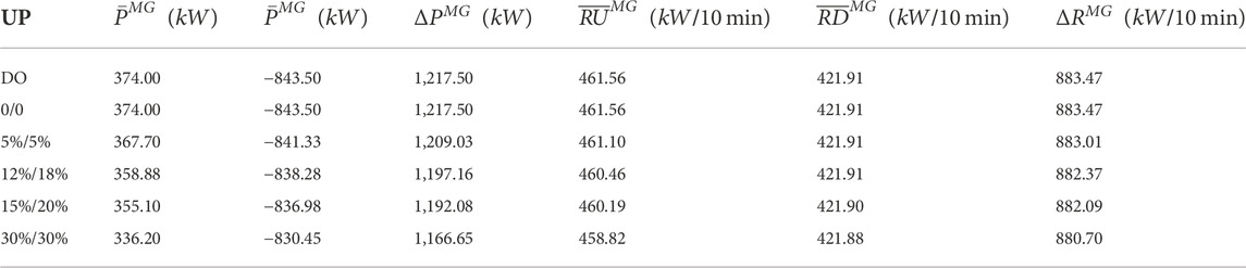
TABLE 4. Results of MG-FPs with different risk preferences in configuration case 1.

It is shown that the MEMG operator’s risk preference does not have much impact on ramping rate flexibility parameters, but is influential on power flexibility parameters. When the UP is set to 0, the ARO model is equal to the DO model, the look-best MG-FPs among these contrast sets are obtained. As UPs increase, MG-FPs tend to get worse to adapt to the worse scenarios. This indicates that the operators will give more consideration to the uncertainty they face when determining MG-FPs. Therefore, the parameters will be more conservative, which means that the MG-FPs of MEMG get worse. Conversely, when the operators consider more about the favorable scenarios, the UPs will be small, resulting in better MG-FPs values.

We can conclude that the evaluated flexibility level of the MEMG system is related to the risk preference of MEMG operators. When the MEMG operator is a conservative idea holder, the submitted MG-FPs are likely to be constrictive. Otherwise, if the MEMG operator is a risk-taker, the MEMG appears to be more effective in supporting the flexible operation of the main network although the actual flexibility capability of MEMG does not change.

In addition to the risk preference of the MEMG operator, the system configuration of the MEMG has a more significant impact on the assessment results. This impact may arise from the characteristics of the MEMG units and the synergies between them. The impact of system configuration on MG-FPs is researched through the following three configuration cases:

Case 1 All units in the MEMG are available in the scheduling.

Case 2 State variables of GT 1 and P2G 1 are set to 0, and other units in the MEMG are available.

Case 3 Only EB 1 and EB 3 are reserved as heat sources of the heat supply network, state variables of other units are set to 0.

The optimization results are presented in Table 5. With the reduction of units in the MEMG system, the flexibility parameters of MEMG become significantly worse in terms of power and ramping rate. The configuration of power-consuming equipment has a significant effect on the minimum power parameter. Because in the MEMG, power-consuming units are regarded as the equivalent electric load, and the minimum power flexibility parameter is limited by the power consumption level. When the power generation equipment in the MEMG system halt, the maximum power parameters will be decreased.

TABLE 5

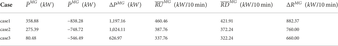
TABLE 5. Results of MG-FPs in different system configuration cases.

4.3 Impact of the prediction error of MEMG operator

To verify that the MG-FPs obtained by the ARO model in this paper can withstand the worst scenarios, the optimization results of the DO model are compared with results of the ARO model in this section. Results of MG-FPs from the two models are presented in Table 6.

TABLE 6

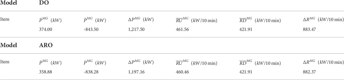
TABLE 6. Results of MG-FPs from different optimization model.

We compare the system’s loss of load (LOL) and RE curtailment rate (RECR) under different prediction errors, as shown in Table 7. The prediction error refers to the degree to which the predicted value of load consumption and available RE deviate from the actual value. The proposed ARO model in the following comparative examples have the same risk preference coefficients of MEMG operator which are 12 and 18% for load and RE, as shown in Figures 6, 7.

TABLE 7

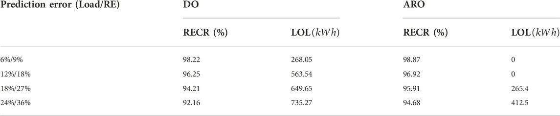
TABLE 7. System operation performance with MG-FPs from different optimization model.

FIGURE 6

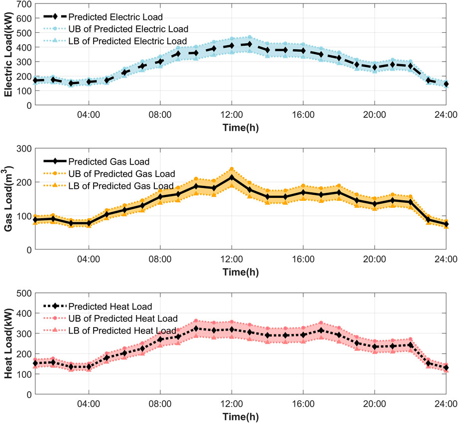
FIGURE 6. MEMG load profiles predicted, and uncertainty intervals.

FIGURE 7

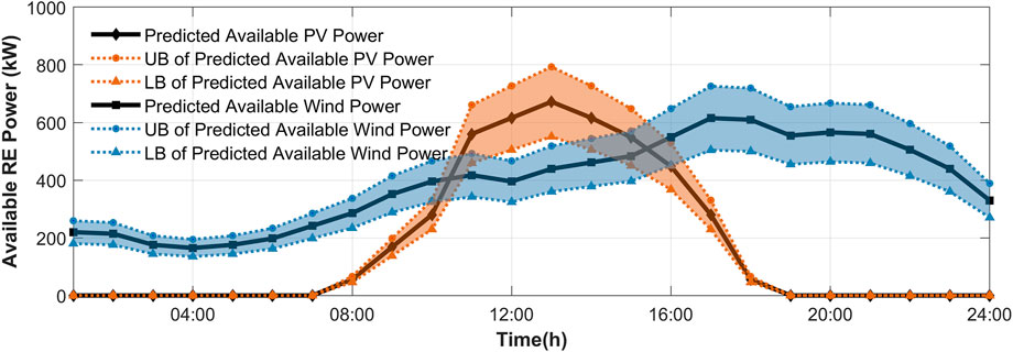
FIGURE 7. MEMG available RE power predicted, and uncertainty intervals.

It should be noted that when solving MG-FPs, MEMG operators do not regard reducible load as a flexible resource that can be curtailed. Therefore, when the prediction error is within the risk preference interval, the MEMGs which submit the MG-FPs of the ARO model will not have load shedding. When the prediction error exceeds MEMG operators’ anticipation (e.g. the power consumption level of MEMG is higher than expected and PDS commands a certain large power output of MEMG, or the available RE output is lower than the lowest expected level), the loads will probably be shed to track the scheduling instructions.

There exists no provision for 100% RE consumption in the ARO model, thus, although the prediction error is expected, RE may not be completely absorbed in MEMG. The rejection of RE power may be due to the constraints of line transmission capacity, the low energy consumption level of MEMG, etc. When the prediction error exceeds the risk tolerance, the RE consumption rate may be further downward constrained by undesirable PDS orders, which are hard to track without RE abandonment (e.g. power instructions of certain low negative values).

The results show that the ARO model has more advantages when considering the prediction error. With the increase in prediction error, the results of the DO method get worse, because the results of DO method are not robust to operational uncertainties. There may occur load shedding or RE abandonment in MEMG, to track the scheduling orders from PDS which are formulated with submitted MG-FPs. The results indicate that the robust optimization framework we proposed to obtain MG-FPs possesses preponderance, especially in scenarios with large prediction error.

5 Conclusion

In this paper, we propose a specific evaluation method for the operational flexibility of distributed MEMG in supporting power distribution systems. The method has the following merits.

The flexibility-oriented model of MEMG is introduced, by systematically considering the flexibility resources of MEMG. The network constraints are considered as well, making the proposed evaluation method more applicable. The flexibility representation way we adopt, namely MG-FPs, determines that the main network can schedule the MEMGs as conventional units or loads in the primal scheduling model. Besides, the privacy problem can be avoided.

Several uncertainties are considered when assessing the flexibility of MEMG, making the assessment result robust. The MG-FPs obtained through the ARO model proposed in this paper can resist the influence of system operational uncertainty to a certain extent, which depends on the prediction error of the uncertainty set and the risk preference of the MEMG operator. The case studies show the effectiveness of the MG-FPs in representing the flexibility of MEMG. It can also be summarized that the flexibility capability of MEMG is related to equipment configuration, line transmission capacity, and energy consumption level.

Future works include 1) improving the model of MEMG components to meet the actual needs; 2) developing a reasonable pricing mechanism for the flexibility of the MEMG to encourage the MEMG to participate in the operation support of the main network.

Data availability statement

The original contributions presented in the study are included in the article/Supplementary Material, further inquiries can be directed to the corresponding author.

Author contributions

JW performed the statistical analysis and wrote the first draft of the manuscript. ZW contributed to the conception and design of the study. All authors contributed to manuscript revision and read and approved the submitted version.

Funding

This research was supported in part by the National Key R&D Program of China under Grant 2020YFE0200400, in part by the National Natural Science Foundation of China under Grant 52177077.

Conflict of interest

The authors declare that the research was conducted in the absence of any commercial or financial relationships that could be construed as a potential conflict of interest.

Publisher’s note

All claims expressed in this article are solely those of the authors and do not necessarily represent those of their affiliated organizations, or those of the publisher, the editors and the reviewers. Any product that may be evaluated in this article, or claim that may be made by its manufacturer, is not guaranteed or endorsed by the publisher.

References

Bahramara, S., Sheikhahmadi, P., Mazza, A., and Chicco, G. (2022). Day-ahead self-scheduling from risk-averse microgrid operators to provide reserves and flexible ramping ancillary services. Int. J. Electr. Power. Energy Syst. 142, 108381. doi:10.1016/j.ijepes.2022.108381

CrossRef Full Text | Google Scholar

Baringo, A., Baringo, L., and Arroyo, J. M. (2019). Day-ahead self-scheduling of a virtual power plant in energy and reserve electricity markets under uncertainty. IEEE Trans. Power Syst. 34 (3), 1881–1894. doi:10.1109/tpwrs.2018.2883753

CrossRef Full Text | Google Scholar

Capuder, T., and Mancarella, P. (2014). Techno-economic and environmental modelling and optimization of flexible distributed multi-generation options. Energy 71, 516–533. doi:10.1016/j.energy.2014.04.097

CrossRef Full Text | Google Scholar

Chen, H., Xuan, P., Wang, Y., Tan, K., and Jin, X. (2016). Key technologies for integration of multitype renewable energy sources—research on multi-timeframe robust scheduling/dispatch. IEEE Trans. Smart Grid 7 (1), 471–480. doi:10.1109/tsg.2015.2388756

CrossRef Full Text | Google Scholar

Chen, X., and Li, N. (2021). Leveraging two-stage adaptive robust optimization for power flexibility aggregation. IEEE Trans. Smart Grid 12 (5), 3954–3965. doi:10.1109/tsg.2021.3068341

CrossRef Full Text | Google Scholar

Chen, X., Wu, W., and Zhang, B. (2018). Robust capacity assessment of distributed generation in unbalanced distribution networks incorporating ANM techniques. IEEE Trans. Sustain. Energy 9 (2), 651–663. doi:10.1109/tste.2017.2754421

CrossRef Full Text | Google Scholar

De Coninck, R., and Helsen, L. (2016). Quantification of flexibility in buildings by cost curves – methodology and application. Appl. Energy 162, 653–665. doi:10.1016/j.apenergy.2015.10.114

CrossRef Full Text | Google Scholar

Dehghan, S., Aristidou, P., Amjady, N., and Conejo, A. (2021). A distributionally robust AC network-constrained unit commitment. IEEE Trans. Power Syst. 36 (6), 5258–5270. doi:10.1109/tpwrs.2021.3078801

CrossRef Full Text | Google Scholar

Ding, T., Li, C., Yang, Y., Jiang, J., Bie, Z., and Blaabjerg, F. (2017). A two-stage robust optimization for centralized-optimal dispatch of photovoltaic inverters in active distribution networks. IEEE Trans. Sustain. Energy 8 (2), 744–754. doi:10.1109/tste.2016.2605926

CrossRef Full Text | Google Scholar

Ding, T., Zhang, X., Lu, R., Qu, M., Shahidehpour, M., He, Y., et al. (2022). Multi-stage distributionally robust stochastic dual dynamic programming to multi-period economic dispatch with virtual energy storage. IEEE Trans. Sustain. Energy 13 (1), 146–158. doi:10.1109/tste.2021.3105525

CrossRef Full Text | Google Scholar

Holjevac, N., Capuder, T., and Kuzle, I. (2015). Adaptive control for evaluation of flexibility benefits in microgrid systems. Energy 92, 487–504. doi:10.1016/j.energy.2015.04.031

CrossRef Full Text | Google Scholar

Holttinen, H., Tuohy, A., Milligan, M., Lannoye, E., Silva, V., Muller, S., et al. (2013). The flexibility workout: Managing variable resources and assessing the need for power system modification. IEEE Power Energy Mag. 11 (6), 53–62. doi:10.1109/mpe.2013.2278000

CrossRef Full Text | Google Scholar

Huang, Z., Zhang, Y., and Xie, S. (2022). Data-adaptive robust coordinated optimization of dynamic active and reactive power flow in active distribution networks. Renew. Energy 188, 164–183. doi:10.1016/j.renene.2022.02.027

CrossRef Full Text | Google Scholar

Jiang, Q., and Hong, H. (2013). Wavelet-based capacity configuration and coordinated control of hybrid energy storage system for smoothing out wind power fluctuations. IEEE Trans. Power Syst. 28 (2), 1363–1372. doi:10.1109/tpwrs.2012.2212252

CrossRef Full Text | Google Scholar

Lannoye, E., Flynn, D., and O'Malley, M. (2012). Evaluation of power system flexibility. IEEE Trans. Power Syst. 27 (2), 922–931. doi:10.1109/tpwrs.2011.2177280

CrossRef Full Text | Google Scholar

Lannoye, E., Flynn, D., and O'Malley, M. (2015). Transmission, variable generation, and power system flexibility. IEEE Trans. Power Syst. 30 (1), 57–66. doi:10.1109/tpwrs.2014.2321793

CrossRef Full Text | Google Scholar

Liu, M. Z., Ochoa, L. N., Riaz, S., Mancarella, P., Ting, T., San, J., et al. (2021). Grid and market services from the edge: Using operating envelopes to unlock network-aware bottom-up flexibility. IEEE Power Energy Mag. 19 (4), 52–62. doi:10.1109/mpe.2021.3072819

CrossRef Full Text | Google Scholar

Lu, Z., Li, H., and Qiao, Y. (2018). Probabilistic flexibility evaluation for power system planning considering its association with renewable power curtailment. IEEE Trans. Power Syst. 33 (3), 3285–3295. doi:10.1109/tpwrs.2018.2810091

CrossRef Full Text | Google Scholar

Lund, P. D., Lindgren, J., Mikkola, J., and Salpakari, J. (2015). Review of energy system flexibility measures to enable high levels of variable renewable electricity. Renew. Sustain. Energy Rev. 45, 785–807. doi:10.1016/j.rser.2015.01.057

CrossRef Full Text | Google Scholar

Ma, J., Silva, V., Belhomme, R., Kirschen, D. S., and Ochoa, L. F. (2013). Evaluating and planning flexibility in sustainable power systems. IEEE Trans. Sustain. Energy 4 (1), 200–209. doi:10.1109/tste.2012.2212471

CrossRef Full Text | Google Scholar

Majzoobi, A., and Khodaei, A. (2017). Application of microgrids in supporting distribution grid flexibility. IEEE Trans. Power Syst. 32 (5), 3660–3669. doi:10.1109/tpwrs.2016.2635024

CrossRef Full Text | Google Scholar

Makarov, Y. V., Loutan, C., Ma, J., and De Mello, P. (2009). Operational impacts of wind generation on California power systems. IEEE Trans. Power Syst. 24 (2), 1039–1050. doi:10.1109/tpwrs.2009.2016364

CrossRef Full Text | Google Scholar

Mancarella, P. (2014). MES (multi-energy systems): An overview of concepts and evaluation models. Energy 65, 1–17. doi:10.1016/j.energy.2013.10.041

CrossRef Full Text | Google Scholar

Martinez Cesena, E. A., Good, N., Panteli, M., Mutale, J., and Mancarella, P. (2019). Flexibility in sustainable electricity systems: Multivector and multisector nexus perspectives. IEEE Electrific. Mag. 7 (2), 12–21. doi:10.1109/mele.2019.2908890

CrossRef Full Text | Google Scholar

Parhizi, S., Lotfi, H., Khodaei, A., and Bahramirad, S. (2015). State of the art in research on microgrids: A review. IEEE Access 3, 890–925. doi:10.1109/access.2015.2443119

CrossRef Full Text | Google Scholar

Shao, C., Ding, Y., Wang, J., and Song, Y. (2018). Modeling and integration of flexible demand in heat and electricity integrated energy system. IEEE Trans. Sustain. Energy 9 (1), 361–370. doi:10.1109/tste.2017.2731786

CrossRef Full Text | Google Scholar

Trovato, V., Teng, F., and Strbac, G. (2018). Role and benefits of flexible thermostatically controlled loads in future low-carbon systems. IEEE Trans. Smart Grid 9 (5), 5067–5079. doi:10.1109/tsg.2017.2679133

CrossRef Full Text | Google Scholar

Ulbig, A., and Andersson, G. (2014). Analyzing operational flexibility of electric power systems. Power systems computation conference: Ieee.

Google Scholar

Ulbig, A., and Andersson, G. (2012). On operational flexibility in power systems. IEEE Power and Energy Society General Meeting: IEEE

Google Scholar

Wang, Q., and Hodge, B.-M. (2017). Enhancing power system operational flexibility with flexible ramping products: A review. IEEE Trans. Ind. Inf. 13 (4), 1652–1664. doi:10.1109/tii.2016.2637879

CrossRef Full Text | Google Scholar

Wang, Y., Cheng, J., Zhang, N., and Kang, C. (2018). Automatic and linearized modeling of energy hub and its flexibility analysis. Appl. Energy 211, 705–714. doi:10.1016/j.apenergy.2017.10.125

CrossRef Full Text | Google Scholar

Wu, X., and Conejo, A. J. (2020). Security-constrained ACOPF: Incorporating worst contingencies and discrete controllers. IEEE Trans. Power Syst. 35 (3), 1936–1945. doi:10.1109/tpwrs.2019.2937105

CrossRef Full Text | Google Scholar

Wu, Y. J., Liang, X. Y., Huang, T., Lin, Z. W., Li, Z. X., and Hossain, M. F. (2021). A hierarchical framework for renewable energy sources consumption promotion among microgrids through two-layer electricity prices. Renew. Sustain. Energy Rev. 145, 111140. doi:10.1016/j.rser.2021.111140

CrossRef Full Text | Google Scholar

Wu, Y., Shi, Z., Lin, Z., Zhao, X., Xue, T., and Shao, J. (2022). Low-carbon economic dispatch for integrated energy system through the dynamic reward and penalty carbon emission pricing mechanism. Front. Energy Res. 10, 843993. doi:10.3389/fenrg.2022.843993

CrossRef Full Text | Google Scholar

Xiang, Y., and Wang, L. (2019). An improved defender–attacker–defender model for transmission line defense considering offensive resource uncertainties. IEEE Trans. Smart Grid 10 (3), 2534–2546. doi:10.1109/tsg.2018.2803783

CrossRef Full Text | Google Scholar

Yan, M., Shahidehpour, M., Paaso, A., Zhang, L., Alabdulwahab, A., and Abusorrah, A. (2021). Distribution system resilience in ice storms by optimal routing of mobile devices on congested roads. IEEE Trans. Smart Grid 12 (2), 1314–1328. doi:10.1109/tsg.2020.3036634

CrossRef Full Text | Google Scholar

Yan, M., Zhang, N., Ai, X., Shahidehpour, M., Kang, C., and Wen, J. (2019). Robust two-stage regional-district scheduling of multi-carrier energy systems with a large penetration of wind power. IEEE Trans. Sustain. Energy 10 (3), 1227–1239. doi:10.1109/tste.2018.2864296

CrossRef Full Text | Google Scholar

Yang, W., Liu, W., Chung, C. Y., and Wen, F. (2020). Coordinated planning strategy for integrated energy systems in a district energy sector. IEEE Trans. Sustain. Energy 11 (3), 1807–1819. doi:10.1109/tste.2019.2941418

CrossRef Full Text | Google Scholar

Zang, H., Cheng, L., Ding, T., Cheung, K. W., Wei, Z., and Sun, G. (2020). Day-ahead photovoltaic power forecasting approach based on deep convolutional neural networks and meta learning. Int. J. Electr. Power. Energy Syst. 118, 105790. doi:10.1016/j.ijepes.2019.105790

CrossRef Full Text | Google Scholar

Zang, H., Xu, R., Cheng, L., Ding, T., Liu, L., Wei, Z., et al. (2021). Residential load forecasting based on LSTM fusing self-attention mechanism with pooling. Energy 229, 120682. doi:10.1016/j.energy.2021.120682

CrossRef Full Text | Google Scholar

Zeng, B., and Zhao, L. (2013). Solving two-stage robust optimization problems using a column-and-constraint generation method. Operations Res. Lett. 41 (5), 457–461. doi:10.1016/j.orl.2013.05.003

CrossRef Full Text | Google Scholar

Zhang, Y., Han, X., Yang, M., Xu, B., Zhao, Y., and Zhai, H. (2019). Adaptive robust unit commitment considering distributional uncertainty. Int. J. Electr. Power. Energy Syst. 104, 635–644. doi:10.1016/j.ijepes.2018.07.048

CrossRef Full Text | Google Scholar

Zhao, J., Wang, J., Xu, Z., Wang, C., Wan, C., and Chen, C. (2017a). Distribution network electric vehicle hosting capacity maximization: A chargeable region optimization model. IEEE Trans. Power Syst. 32 (5), 4119–4130. doi:10.1109/tpwrs.2017.2652485

CrossRef Full Text | Google Scholar

Zhao, J., Zheng, T., and Litvinov, E. (2016). A unified framework for defining and measuring flexibility in power system. IEEE Trans. Power Syst. 31 (1), 339–347. doi:10.1109/tpwrs.2015.2390038

CrossRef Full Text | Google Scholar

Zhao, J., Zheng, T., and Litvinov, E. (2015). Variable resource dispatch through do-not-exceed limit. IEEE Trans. Power Syst. 30 (2), 820–828. doi:10.1109/tpwrs.2014.2333367

CrossRef Full Text | Google Scholar

Zhao, L., Zhang, W., Hao, H., and Kalsi, K. (2017b). A geometric approach to aggregate flexibility modeling of thermostatically controlled loads. IEEE Trans. Power Syst. 32 (6), 4721–4731. doi:10.1109/tpwrs.2017.2674699

CrossRef Full Text | Google Scholar