Design and performance analysis of a charge controller for solar system using MATLAB/SIMULINK

The energy utilization of a Photovoltaic (PV) module is determined by the maximum power the module harnesses from the sun. A static PV module can only harness maximum power from the sun at a particular time in a day as the sun revolves. This simply means that if the PV module can be designed to move in such a direction to harness maximum power from the sun, then its energy utilization efficiency will be highly improved over the period the Sun is available. This design can be achieved by employing Perturb and Observe (P and O) algorithm for maximum power point tracking (MPPT). In this study, Propotional and Integral (PI) controller along with P and O is proposed to solve the problem of low efficiency and irregular output oscillations. The simulation is carried out in the MATLAB/SIMULINK environment and the result shows that by incorporating the PI controller into the system, the efficiency of 99.96% at the maximum power point was attained.

1 Introduction

For years the Sun has provided the earth with a great abundance and replenishable energy, this energy is called solar energy. The amount of solar energy delivered in one second is proportional to the earthquake that occurred in 1906 which had a magnitude of 7.8 (which is approximately 10¹⁷ J), which proves that the earth has a large amount of energy at its disposal. Solar energy is categorized as renewable (non-conventional) energy, it is inexhaustible, replenishable, and readily available (Hayat et al., 2019; Timilehin F et al., 2019). Solar energy is clean and has zero carbon emission, At the Earth’s surface, its intensity is relatively minimal, primarily due to the vast radial spread of radiation from the far Sun (Falayi et al., 2017; Oyedepo et al., 2021). Several technologies have been developed to fully harness solar power, these include: photovoltaics-which converts photons into electrons for electricity; concentrated solar power-which utilizes heat from the Sun; and solar heating and cooling systems which provide hot water and air conditioning. This study focuses critically on how to extract maximum energy from the Sun through PV technology.

The concept of the PV effect propounded by Edmund Becquerel was initially discussed in 1839 (Jungbluth et al., 2012). The first ever solar cell (a unit of PV) manufactured from silicon was produced in the year 1954. Photovoltaics (PV) has a short history compared to conventional sources of electricity. By definition, a photovoltaic device is a device designed to generate electrical power straight from sunlight through an electronic process that occurs only in semiconductor materials. PV arrays arise from a combination of solar cells; each solar cell receives photons from the Sun which ionizes the semiconductor material allowing outermost electrons to be freed from their atomic bonds. Because of the nature of the semiconductor, these outermost electrons are compelled to flow in a unidirectional path leading to the creation of electricity. The knowledge of semiconducting materials has brought about the development of different solar cell configurations for PV modules which include; single-crystalline silicon cells, multi-crystalline silicon cells, ribbon silicon cells and amorphous silicon cells (Jungbluth et al., 2012). Single-crystalline cells perform best at very high irradiance and temperature conditions, they also require a very little amount of space compared to other types and also have a longer lifespan. The multi-crystalline solar cells are relatively cheaper and are faster to manufacture, their heat tolerance is low compared to their counterparts and silicon is not usually wasted during its manufacturing process (Koynov et al., 2007). The ribbon silicon cells use only half the amount of silicon for the manufacturing of single-crystalline which makes it more affordable but reduces its efficiency (Kim et al., 2003). The amorphous silicon solar cells are very cheap, considered the lightest type of cells and have a very high potential (Zeman and Schropp, 1995). PV array systems can serve both domestic and industrial purposes. In terms of domestic purposes, it helps to power light bulbs in houses, fans, etc. In terms of industrial purposes, PV arrays are incorporated into the grid network to provide distributed generation (DG). To extract this power from the PV, the charge controller was invented to regulate energy being absorbed from the Sun through the PV system which comprises a solar panel, charge controller, battery, and inverter.

A charge controller or charge regulator is a voltage and/or current controller (Osaretin and Edeko, 2015). It stabilizes the current and voltage extracted from the PV array which will be used to power loads and or charge batteries. If there is no charge controller, the power will not be regulated to suit the power quality of the battery or the load and this will reduce the battery life span and or damage the connected loads. Different software has been adopted to design and simulate various charge controller configurations before manufacturing them. Popular software used for solar charge controller designs in MATLAB/Simulink. The development of this technology has made most controller designs done on MATLAB based on maximum power point tracking (MPPT) (Teja Manne and Sy, 2018). MPPT is an approach that works with variable power sources to maximize the energy extraction as temperature and irradiance vary. Hence, in this study, an MPPT algorithm called the Perturb and Observe has been adopted to control the behaviour of PV arrays in conjunction with the charge controller.

The process of integrating solar photovoltaic (PV) power into the national utility grid is known as solar grid integration. With rising demand for alternative clean energy sources and increasing global generation capacity of solar power, solar grid integration is becoming more common around the world. There are two types of grid-connected solar generation: distributed generation (small residential and commercial renewables typically range between 5 and 500 kW) on the distribution grid where electricity load is served, and centralized, utility-scale generation (hundreds of megawatts of power) on the transmission grid where electricity load (both linear and non-linear) is served. The explosive growth of non-linear loads caused by power electronic switching in magnetic ballasts and light emitting diodes is affecting utility grid power quality. These loads introduce harmonic currents to flow through the grid (Nazir et al., 2020). This makes it difficult for the integration of PV modules into the grid network, in order to inject balanced positive sequence currents into the grid, the fundamental positive sequence component must be extracted from the polluted load current. There are various techniques required to control the grid-connected PV system interfacing inverter. Because of its robustness and simplicity in implementation, the second order generalized integrator (SOGI) is the most widely used control technique (Han et al., 2015). In (Nazir et al., 2020), an enhanced second order generalized integrator (ESOGI) based control technique was initiated. The proposed ESOGI is used to extract fundamental components from dysfunctional grid voltages and nonlinear load currents. This integrator proficiently addresses the traditional SOGI’s DC offset, inter-harmonic, and integrator delay issues. This control technique also includes power factor correction, harmonic elimination, and load balancing capabilities (Nazir et al., 2020). The ESOGI controller generates reference grid currents that are used to control the voltage source converter (VSC), which connects the PV panel to the grid. In (Han et al., 2015), another PV grid integration technique was adopted which is referred to as the gradient descent least squares regression (GDLSR) based neural network (NN). This method addresses the issues associated with the old adaptive control approaches which are; These algorithms’ performances are not examined under abnormal grid conditions, which are the most common, odd, and critical phenomenon in distributed power generation systems. The major advantages of this grid integration control technique is the derivative term is removed, the computational burden is reduced, and its performance control is instantaneous and suitable for high-frequency systems (Han et al., 2015). In (Kumar et al., 2019a), a Multi-Objective Grid Integrated Solar PV Based Distributed Generating (DG) System was proposed which uses a power normalized kernel least mean fourth algorithm based neural network (NN) control (PNKLMF-NN) technique and learning based hill climbing (L-HC) MPPT (Maximum Power Point Tracking) algorithm. This L-HC algorithm is an improved version of the Hill Climbing (HC) algorithm (Kjær, 2012), which addresses the inherent flaws of conventional HC algorithms such as steady state perturbation, slow dynamic responses, and fixed step size difficulties. The proposed L-HC algorithm has a simple structure that is straightforward to implement, and its learning nature specifies the size of the step change depending on the situation, such as step size decreases during steady state conditions and step size increases during dynamic changes. The combination of the normalized power kernel trick and the least mean fourth (LMF) algorithm gives rise to the PNKLMF-NN algorithm (Kjær, 2012). The normalized power kernel trick realizes the linear relationship between the input signal and the High-Dimensional Space during mapping (HDS). Mapping in HDS technique is used to improve accuracy with the help of power kernel trick. The least mean fourth algorithm is used to minimize internal errors. Another advantage of the PNKLMLF-NN algorithm is that the input signals can smoothly map into the HDS without prior knowledge of the coordinates (Kjær, 2012). Authors in (Kumar et al., 2019b) hybridize a novel ANOVA Kernel Kalman Filter (AKKF)-based adaptive control algorithm with the conventional p&O mppt algorithm. The AKKF is an improved version of the Kalman Filter (KF), in which the ANOVA Kernel (AK) trick is used to improve the KF’s estimation accuracy. AKKF is a member of the affine projection family, and the ANOVA kernel function is used to quickly identify the fundamental component of an input signal. The algorithm delay, logic complexity, and computational burden are significantly reduced in this case due to the hybridization of kernel trick and gradient vector with Kalman Filter (Kumar et al., 2019b). In (Singh et al., 2020), a P and O based MPPT algorithm is used in conjunction with the steepest descent Laplacian regression (SDLR) based adaptive control technique. This technique is a hybrid of the affine projection family’s steepest descent vector and least fourth regression. Furthermore, the Laplacian kernel function is used here for quick pattern recognition as well as to improve filter performance. A unique feature of this control technique is that during the night, or when solar PV power generation is zero, the voltage source converter (VSC) and DC-link capacitor function as a Distribution Static Compensator (DSTATCOM), providing reactive power support to the grid (Singh et al., 2020).

In ref. (Mohapatra et al., 2019), the authors carried out a comparative analysis between a conventional and adaptive P and O MPP tracker. The proposed p&O tracker was implemented to increase tracking speed and minimize steady state oscillations. In order to speed up the tracking speed, perturbations on current were considered over voltage. The KC200GT PV module is designed to measure maximum voltage, current and power values of 51.8 V, 3.92 A, and 201.5 W respectively. The controller adopted is a robust hysteresis band current (HCC). The DC-DC step up chopper is designed with an Insulated Gate Bipolar Transistor (IGBT), capacitor (330 μF), inductor (2 mH), Vin= (0–100 V) and Vout = 300 V. the switching frequency of the converter was set to 20 KHz. At maximum power point, the time to reach steady state oscillation was recorded to be 0.75 s. The conventional method is designed to track maximum power in 13,8 s. During the experimentation phase, a PV Emulator is used in place of the PV module, a physical boost converter with a microcontroller and Digital Storage Oscillator (DSO) is used instead of the HCC (which has not been implemented in the real word). Since the HCC did not have a direct equivalent during the experimentation stage, it is seen as the major drawback in the paper.

In ref. (Anowar and Roy, 2019), the author developed a solar MPPT charge controller based on incremental conductance with MATLAB/Simulink. It was noticed that the conductance algorithm tracks maximum power but at low efficiencies due to the presence of oscillations. The methodology requires the observation that the first derivative using the product rule of the PV function is zero at the maximum point, which implies that the differentiation of the power concerning the voltage is zero (dp/dv = 0). From power = voltage*current (p=I*V) and this power depends on voltage which makes it p=(I*V) *V. Using the product rule to differentiate the expression and equating it to zero the author obtained dI/dV = -I(V)/V which is regarded as the maximum power point (MMP) i.e., when the increment conductance is equal to negative instantaneous conductance. The PV framework is demonstrated in the MATLAB/Simulink platform. The conventional Simulink PV model is utilized. The solar panel is connected to the battery through a Direct Current to Direct Current (DC) boost converter. 15mH inductance, 100F input capacitance, 2200F output capacitance, and frequency switching at 5 kHz are used in the boost converter. The integral regulator adds the instantaneous error to the controller output after multiplying it by the integral gain. The source impedance must be equivalent to the output impedance to accomplish maximum power. The greatest power can be attained by adjusting the DC-DC converter duty cycle, which matches the source and output impedance. At the end of experimentation, under comparative analysis between the system with and without the MPPT, the output power for the proposed MPPT is 45% higher than the system without MPPT. The oscillation also decreased to the extent that there was a stable output. Lastly, with the MPPT the system can accommodate both Lead-acid and Lithium-ion batteries but in the case of the system without MPPT, only Lead-acid batteries can be used. It has low efficiency because a controller was not embedded into the system to prevent irregular oscillations.

In ref. (Anowar and Roy, 2019), the author developed a derated mode of power generation in PV Systems using the P and O algorithm. The conventional P and O analysed in the paper made use of a boost converter which consist of a switch, diode, inductor and capacitor in order to provide the required voltage level to power the load. The proposed controller revolves around the functionality of the duty cycle using the three-stage control strategy which considers PV array voltage readings of V_PV(k), V_PV(k-1), V_PV(k+1) (where k refers to the selected operation point on the P-V characteristic curve). The 3-stage approach considers the left (before the maximum powerpoint) and right (after the maximum powerpoint) operation regions of the P-V characteristic curve. In the left region, mathematically, the slope (dp/dv > 0) is positive which means the system will move forwards towards MPP (dp/dv = 0). In the right region, mathematically, the slope (dp/dv < 0) is negative which means the system will move backwards towards MPP. The boost converter duty cycle is a function of the ratio of power to voltage changes (dp/dv). It was also determined that the ratio of the output dc voltage to the output dc current provided the output impedance which will serve as a link to power the load. Considering the change in the step size (ΔD), the smaller its value, the longer it takes to achieve MPP which will lead to low efficiency. However, the larger its value, the shorter it takes to achieve MPP which will lead to high efficiency. The paper chose a small step size of duty ratio (ΔD = 3 × 10-7) and a big step size (ΔD = 3 × 10-4) for the sake of evaluation and due to the large step size, there was significant oscillation in the input voltage. As a result, it can be concluded that a large step size can achieve a fast dynamic response. However, due to the large step size, the operation point oscillates near the MPP.

Authors in (Argyrou et al., 2018) modelled a PV system which comprises different MPPT techniques using MATLAB/Simulink. The article aimed to design both a P and O and IC MPPT type algorithm and compare both with the fuzzy logic control to improve the efficiency of both algorithms. The system consisted of a PV array with the capacity of 250 W with 60 cells connected in series. The P and O algorithm focused on the changes to the reference voltage. During the simulation, the initial step size of the reference voltage was defined to be 0.5 V. It was noticed that 0.5 V would not be sufficient enough to meet up the tracking time of the fuzzy logic MPPT-based controller. The solution to this was to increase the step size to 1.5 V. However, the increment to the step voltage would result in more irregular oscillations in conjunction with limited accuracy and efficiency.

In ref. (Argyrou et al., 2018; Tan et al., 2020), the authors modelled and simulated a P and O based MPPT lead acid battery controller for standalone sytsems in MATLAB. The system consisted of two main blocks; the P and O MPPT tracker and the three-stage battery charger. The controller is designed to produce a Pulse Width Modulated signal (PWM). The PWM is used to drive the DC-DC converter into on and off state via the transistor which acts as a switch. The proposed model has the ability to charge 48 V battery from a 2000 W PV module. The DC-DC coverter is a step down one that converts the input voltage from the PV to a low ouput voltage. The design specifications of the buck converter are as follows; schottky diode of forward voltage 0.5V, MOSFET of switching frequency 1KHz, input voltage of 120 V, duty ratio of 0.4, inductor ripple current of 0.288 mA and output capacitive ripple voltage of 2.3 nV. The p&O algorithm works on the basis of trial and error but perturbation is performed on the duty cycle when power detected varies. The implementation of the P and O algorithm required the use of Simulink blocks instead of a scripted code. In the paper, the model of the proposed system has been successfully simulated in the MATLAB/Simulink environment. The Simulink model was designed using ode23 tb (Stiff/TR-BDF2) solver with a variable step signal. It was observed from the efficiency curve that the highest efficiency attainable from the solar charge controller was 99.9% at an irradiance of 300 W/m2 which would track approximately 579W.

Authors in (Ahmed and Salam, 2018) implemented a p and O-based MPPT technique using MATLAB/Simulink. The solar cell of the system was modelled mathematically with the use of a double-diode set up in MATLAB. The algorithm works based on small perturbation increments to attain maximum output power. The first power measured is P_K which is obtained from the measurements of both V_K and I_K of the solar array. ΔV is added as a form of small perturbation. Then P_K+1 is obtained from the new values of V_K+1 and I_K+1, if P_K+2 reads positive then the controller maintains perturbation in the same particular direction (P_K+3 P_K+4 P_K+5 and so on). Once P_K+1 gives a negative value, the algorithm returns the system to maximum power by introducing a negative increment. When the maximum power point is reached, the system operating point begins to oscillate constantly around it. The controller will monitor this operating point and attempt to bring the solar module’s V to this maximum power point. In this case, the controller would be in a DC-DC converter located along the DC module output. The model is quite complex which will in turn makes its implementation expensive. The work done by researchers concerning maximum power tracking by solar cells has shown that Perturb and Observe algorithm is very useful in that aspect. However, gaps still exist. One of which is the irregular output. Hence, in this paper, the redefined duty cycle is used alongside Perturb and Observe algorithm in the design of the solar panel charge controller to achieve regular output.

2 Materials and methods

The design of the maximum power tracking solar charge controller is carried out in MATLAB and the following components are required in the Simulink design: PV array; Lead-acid Battery; PI controller; Boost Converter; Inductor; Output capacitor; Input Capacitor; and Metal Oxide Semiconductor Field Effect Transistor (MOSFET).

2.1 System design

The design of the solar panel charge controller system using Perturb and Observe algorithm and PI controller is software based. However, the values and ratings of parameters required are determined through already established theories.

2.1.1 Modelling of photovoltaic array

The equivalent simplified circuit diagram of a solar cell is represented by a current source connected in shunt to a diode. Ideally, this model is completed with the use of resistors to represent the losses and sometimes with other additional diodes that take into account other phenomena (Wolf and Rauschenbach, 1963). This brings about the equivalent circuit for the PV array is shown in Figure 1. It consists of a current source, diode, shunt resistor and series resistor. Every solar panel has its data sheet which consists of the calculated parameters which will be used for further design analysis. The electrical parameters to be determined from the circuit are short-circuit current (I_SC), open circuit voltage (V_OC), current at maximum power point (I_mp) and voltage at maximum power point (V_mp).

FIGURE 1

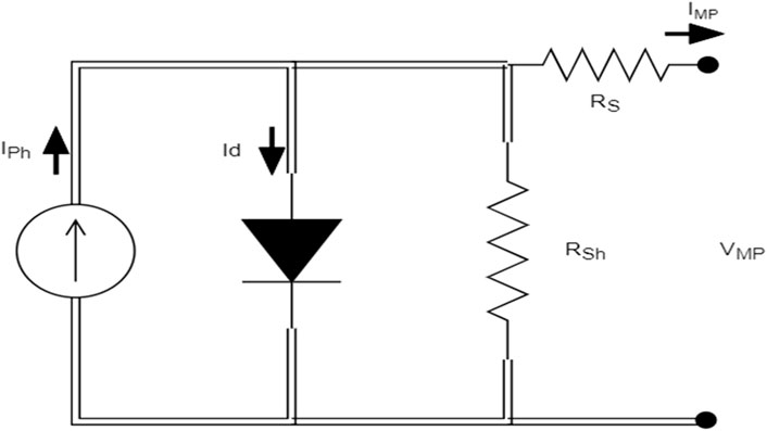
FIGURE 1. The equivalent circuit for PV array.

Current at maximum power point I_mp is obtained using Kirchhoff’s Current Law,

$i_{mp}=i_{ph}-i_d-i_{Rsh}(1)$

where

$i_d=i_o\left(e^{\left(\frac{q\left(V_{mp}+I_{mp}{R}_s\right)}{\propto KT}\right)}-1\right)$

and

$i_{Rsh}=\frac{V_{mp}+i_{mp}{R}_s}{R_{sh}}$

then

$i_{mp}=i_{ph}-i_o\left(e^{\left(\frac{q\left(V_{mp}+I_{mp}{R}_s\right)}{\propto KT}\right)}-1\right)-\frac{V_{mp}+i_{mp}{R}_s}{R_{sh}}(2)$

where V_mp is given as:

$V_{mp}=V_{T}In\left(\frac{i_{ph}}{i_o}\right)-In\left(\frac{V_{mp}}{V_T}-1\right)(3)$

Short-circuit current I_sc is obtained by shorting the circuit which results in V_mp = 0 and I_SC > I_mp.

$i_{sc}=i_{ph}-i_0\left(e^{\left(\frac{q\left(0+i_{sc}{R}_s\right)}{\propto KT}\right)}-1\right)-\frac{0+i_{sc}{R}_s}{R_{sh}}(4)$

$i_{sc}=i_{ph}-i_0\left(e^{\left(\frac{q\left(i_{sc}{R}_s\right)}{\propto KT}\right)}-1\right)-\frac{i_{sc}{R}_s}{R_{sh}}(5)$

Open circuit voltage V_oc is obtained when I_mp = 0 and V_oc > V_mp.

$0=i_{ph}-i_o\left(e^{\left(\frac{q\left(V_{oc}\right)}{\propto KT}\right)}-1\right)-\frac{V_{oc}}{R_{sh}}(6)$

$V_{oc}=n{V}_{T}In\left(\frac{i_p+i_o}{i_o}\right)(7)$

Maximum Power is given as:

$P_{mp}=i_{mp}{v}_{mp}(8)$

where;

$i_{ph}$ = light or photon current at a given irradiance at a given temperature = 8.9523 A

$i_d$ = Diode current

$i_0$ = Reverse saturation current of diode = 2.6466 * 10⁻¹⁰ A

q = Charge of an electron = 1.60217662 × 10⁻¹⁹ coulombs.

K = Boltman’s constant = 1.38064852 × 10⁻²³ m² kg⁻² k⁻¹

T = Temperature in Kelvin = 298 K (25°C).

α = Diode ideality factor = 1.0345.

$V_T$ = Thermal Voltage of array = $\frac{\alpha KT}{q}$ = 0.265892

$i_{Rsh}$ = current through shunt resistor

$R_{sh}=\mathrm{S}\mathrm{h}\mathrm{u}\mathrm{n}\mathrm{t}\mathrm{r}\mathrm{e}\mathrm{s}\mathrm{i}\mathrm{s}\mathrm{t}\mathrm{a}\mathrm{n}\mathrm{c}\mathrm{e}\mathrm{v}\mathrm{a}\mathrm{l}\mathrm{u}\mathrm{e}$ = 108.7053 ohms

$R_s=$ $\mathrm{S}\mathrm{e}\mathrm{r}\mathrm{i}\mathrm{e}\mathrm{s}\mathrm{r}\mathrm{e}\mathrm{s}\mathrm{i}\mathrm{s}\mathrm{t}\mathrm{a}\mathrm{n}\mathrm{c}\mathrm{e}\mathrm{v}\mathrm{a}\mathrm{l}\mathrm{u}\mathrm{e}=0.27216\mathrm{o}\mathrm{h}\mathrm{m}\mathrm{s}$

Table 1 shows the electrical parameters extracted from the PV array.

$Rated{P}_{input}=No.ofseriesconnectedmodules*no.ofparallelmodules*P_{mp}$

$RatedInputPower=1*1*259.436=259.436Watts(9)$

TABLE 1

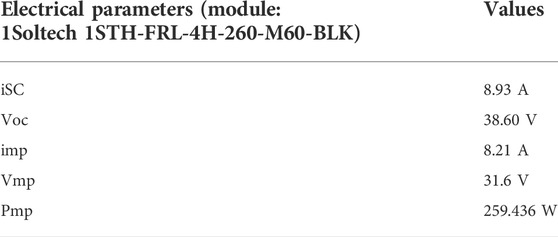
TABLE 1. PV array specifications and calculations.

2.2 boost converter circuit

The boost converter is a circuit designed to step up an input pulsating voltage of approximately 31 V from the PV array to a constant output voltage of approximately 50 V. It consists of a MOSFET being driven by a PWM signal of 0.37125 (37.13%) duty cycle, switching frequency of 2000 Hz, and 10-ohm output resistance. The MOSFET was employed to reduce losses and it has a higher switching time compared to that of other transistors like the IGBT (Insulated-gate bipolar transistor). The duty cycle is obtained using the following equations (Anto et al., 2016).

$D\left(dutycycle\right)=1-\frac{V_{in}}{V_{out}}(10)$

$D\left(dutycycle\right)=1-\frac{31.5}{50.1}=0.37125=37.13\%$

The inductor is connected in series with the input voltage which will build up a magnetic field in the process. The minimum inductance is obtained as follows:

$L_{\min }=\frac{D\left(1-D\right){\hspace{0.17em}}^2\left(R\right)}{2f}(11)$

$L_{\min }=\frac{\left(0.37125\right){\left(1-0.37125\right)}^2\left(10\right)}{2*2000}=3.1669*{10}^{-4}H=0.3167mH$

In boost converter calculations, the minimum inductance is not what is used in the proposed system, the ideal inductance should be 25% larger than the minimum inductance.

$L=1.25*L_{\mathit{min}}=1.25*3.1669*{10}^{-4}=3.9586mH$

The output CAPACITOR can be calculated using:

$r=\frac{∆V_O}{V_O}(12)$

$r=\frac{∆V_O}{V_O}=0.414$

$C=\frac{D}{Rrf}(13)$

$C=\frac{0.37125}{10*0.414*2000}=4.483695*{10}^{-5}=0.0484mF$

Figure 2 shows the simple circuit design for the boost converter circuit which input and output voltages are approximately 31 and 50 V dc respectively.

FIGURE 2

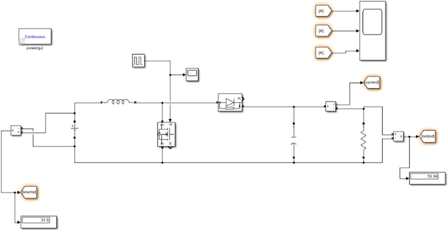
FIGURE 2. Boost converter circuit for PV array.

2.3 PI controller mechanism

The PI controller with the aid of the repeated sequence block and the output response from the perturb and observe algorithm block produces the refined pulse width that powers the MOSFET. Ziegler Nichol’s tuning method was adopted to tune the PI controller. To achieve PI tuning, the gain values of the PI controller must be determined which are K_P (proportional) and K_I (Integral), to achieve these constants, they both must be set to zero. While monitoring the output of the boost converter, the proportional gain (K_P) is increased (while keeping K_I at 0) to a value that forces the boost converter output to oscillate at an approximately constant amplitude; this is called the critical gain (K_cr = 0.45) and the period of the waveform is also noted as T_U. The values of both K_P and K_I were determined subject to the output voltage of 50 V. In Figure 3 the waveform for the critical gain is shown and in Figure 4, the control settings for the PI controller to determine the critical gain; proportional and integral constants are shown.

FIGURE 3

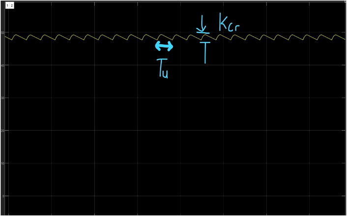
FIGURE 3. Waveform to determine critical gain.

FIGURE 4

FIGURE 4. Initialization of Gains in the PI controller.

The period of oscillation was determined on the software to be $3.10666x{10}^{-3}$ seconds (Tu) and the critical gain (K_cr) is 0.45. To determine the values of the proportional and integral values, the following equations developed by Ziegler Nicholas are used.

$K_P=0.45x{K}_{Cr}=0.45x0.45=0.2025$

$K_I=\frac{0.54X{K}_{Cr}}{T_U}=\frac{0.54x0.45}{3.10666x{10}^{-3}}=78.21889$

These values were input into the (Proportional Integral and Derivative) PID autotuner interface. The simulation was played and it drove the circuit to a 99.975% accuracy. The voltage, current and power readings are varied at ± 0.5 which is very ideal.

The flow chart in Figure 5 shows the process of the entire design to produce a maximum power of approximately 260 Watts, a voltage of 31 V, and a boost converter that steps up the 31V–50 V to charge the battery. With the PI controller controlling the functionality of the MPPT.

FIGURE 5

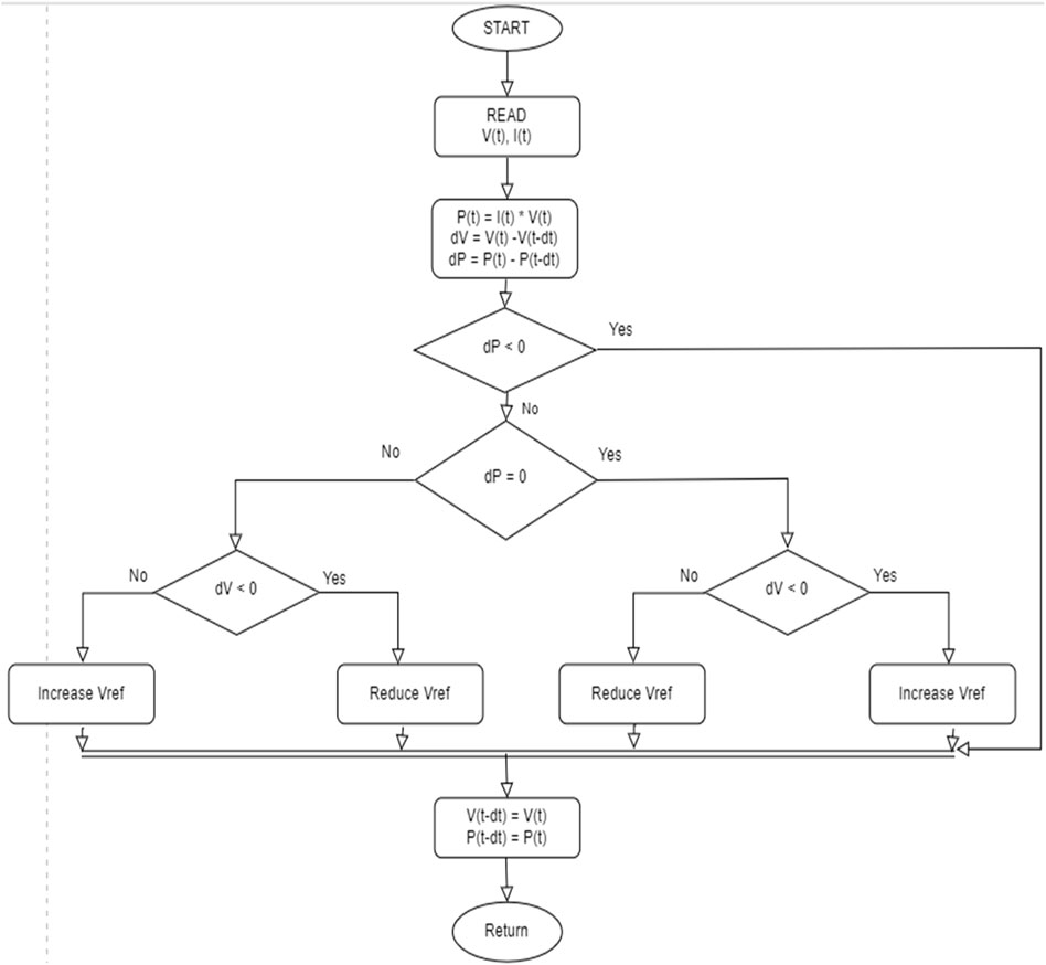
FIGURE 5. Flowchart representing perturb and observe algorithm.

2.4 System functionality

The system consists of the PV array (260W), PI controller, boost converter (31V—50 V) and Lead Acid battery (48 V) which was simulated on MATLAB R2020a (9.8.0.1323502) 64-bit (win64) software. The PV array was designed to accept a step input irradiance function (which means the irradiance varies at different instants of time) and a constant temperature of 25°C. The PV tracking algorithm (P and O) uses the changes in power and voltage values (ΔP and ΔV) which serve as the basis of its operation to achieve optimum tracking. Three scenarios are established. First, when ΔP and ΔV are greater than zero (0), the reference voltage increases which means that the changes in power and voltage must decrease to attain maximum tracking. Second, when ΔP and ΔV are less than zero (0), the reference voltage decreases which means that the changes in power and voltage must increase to attain maximum tracking. And the third scenario is when both ΔV and ΔP are equal to zero, which means maximum tracking is attained (meaning the Maximum power requirement of the PV array is obtainable). Figure 5 indicates the flow chart for the MPPT behaviour using Perturb and Observe algorithm.

The PI controller uses the MPPT algorithm to analytically control the variations in power and voltage for maximum tracking. Making use of the proportional and integral constants (Kp and Ki) of the controller, these sets of values/constants control the voltage and power readings from the PV array. The output response from the PI controller is modulated by a frequency repeating sequence to produce a unique kind of Pulse Width Modulated signal which will be used to drive the gate terminal of the MOSFET (the plant).

The PV array will inject a pulsating dc voltage which will be brought relatively constant by a filtering capacitor. The boost converter receives this voltage (which acts like a voltage source) and its resultant current. At the boost converter circuit, the MOSFET undergoes an ON and OFF behaviour. During the OFF state, the MOSFET acts as an open circuit meaning the inductor is now in series with the diode (which is in forward bias). During the ON state, the signal source goes high and the MOSFET is then short-circuited. The resulting current is diverted through the MOSFET. As time progresses, the inductor becomes like a voltage source (because of the buildup of magneto motive forces) in series with the input voltage. This makes the anode of the diode have a higher potential than its cathode. The output capacitor now charges to a voltage which is greater than the input supply voltage thus successfully confirming the operational functionality of the boost converter.

The battery connected to the system is a 48 V lead acid battery which will be charged by a steady output voltage of 50 V. From the charging characteristics, negative power indicates that the battery is charging while positive power indicates the discharging process. From the system, there are scopes connected at each point of the system to analyze the electrical characteristics of the branches. Figure 6 shows the block diagram of the system and the flow of electrical parameters.

FIGURE 6

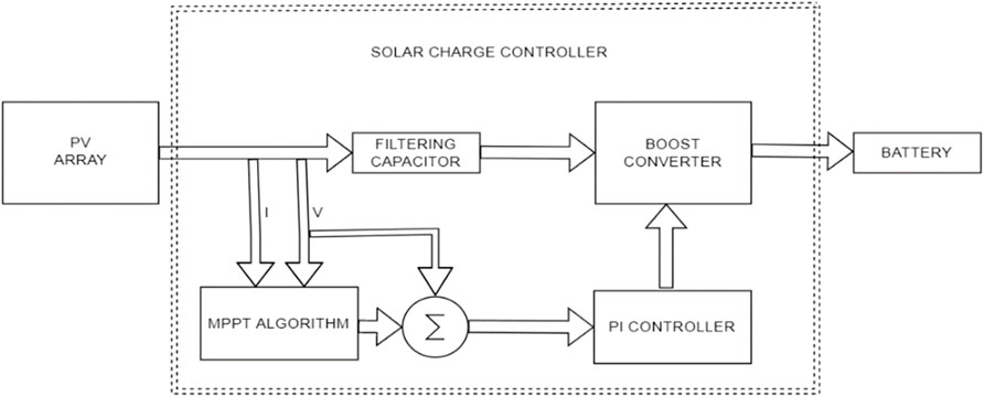
FIGURE 6. System block diagram.

3 Results and discussion

Figure 7 describes the voltage/current and power/voltage characteristics at different irradiance readings from the PV array. The module PV array type selected is a 1Soltech 1STH-FRL-4H-260-M60-BLK which MATLAB integrated specific modifications into its setup. The irradiance values are calibrated in KW/m² and verify the functionality of the array on the graph. At 1000 irradiance (maximum power occurs), the current reading is 8.21A while the voltage is 31.6 V. From the graph, at the 0 V reading the current reads 8.93A which is the short circuit current while at the 0A reading, the voltage reads 38.6 V which is the open-circuit voltage of the PV module. The next display in Figure 7 illustrates how the change in voltage and power varies graphically. At 1000 irradiance, the maximum output power is given as 259.4 Watts with the voltage of 31.6 V and this varies as the irradiance varies. The open-circuit voltage can also be determined when the power from the array is 0 Watts. Table 2 gives a summary of the PV module characteristics such as its open circuit voltage, maximum power at 1000 irradiance, maximum current at 1000 irradiance and short circuit current.

FIGURE 7

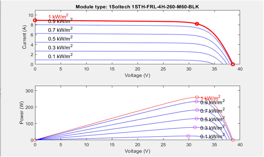
FIGURE 7. Current vs. Voltage and Power vs. Voltage Characteristics.

TABLE 2

TABLE 2. Solar panel parameters.

Table 3 gives a summary of the system characteristics when subjected to physical quantities. At the lowest irradiance value (100W/m²), the system receives a 6.993 W and 0.8247A and outputs a constant voltage of 7.965 V and a current of 0.7460A. At maximum irradiance (1000W/m²), the system receives a maximum voltage and current of 31.46V and 8.261A and produces a constant voltage of 50.01 V and a current of 5.1760A. This verifies the functionality of the boost converter to produce a greater voltage and a far smaller current compared to the input. The simulation time used to carry out this simulation is 2 s. Figure 8 gives a graphical representation of the relationship between irradiance and output voltage for the boost converter which gives a positive slope.

TABLE 3

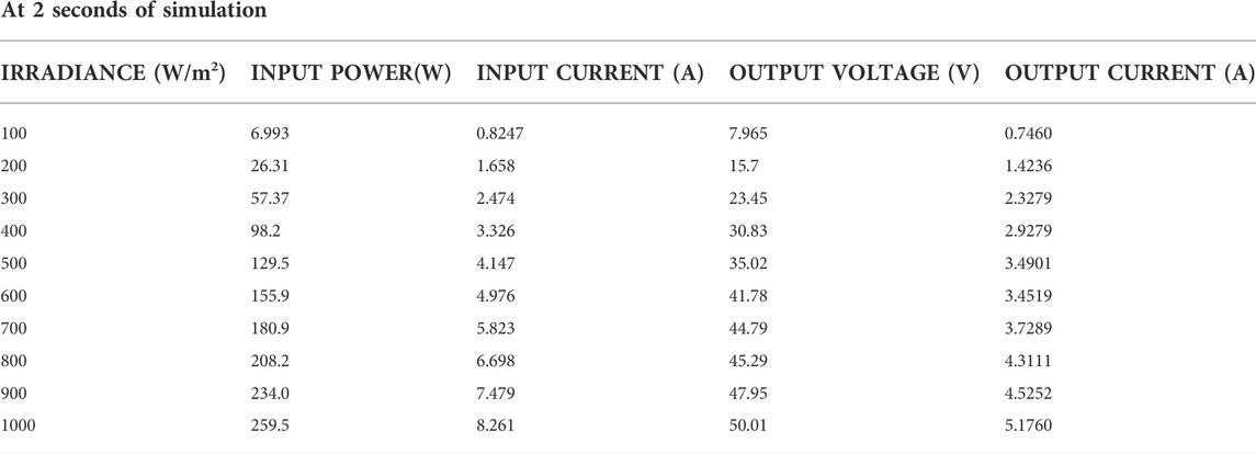
TABLE 3. Readings obtained from the PV array and boost converter.

FIGURE 8

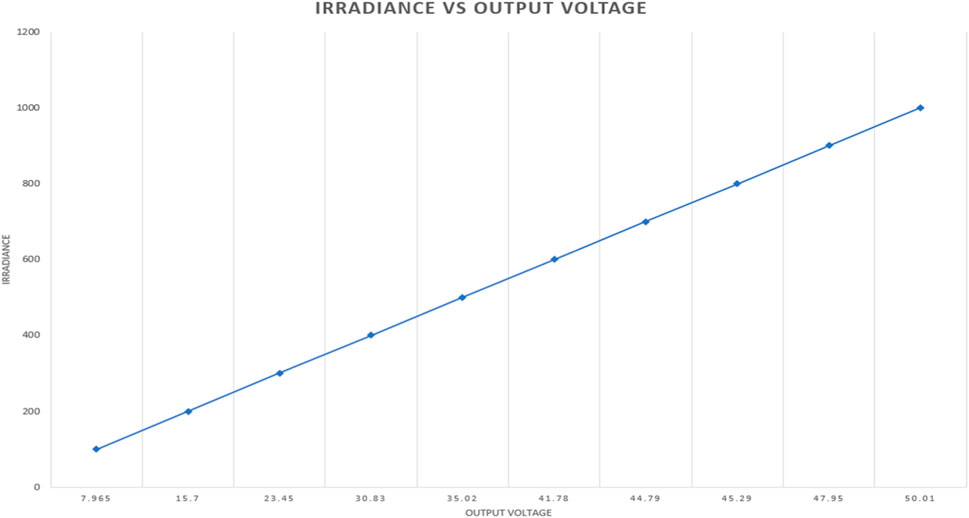
FIGURE 8. Solar irradiance versus output voltage of boost converter.

Table 4 illustrates how the input power to a PV array and the output voltage of the boost converter varies with temperature change. As seen from the table, as temperature increases, the input power decreases which in turn reduces the output voltage from the boost converter required to charge the battery or power the load, this is because, from normal electrical analysis, an increase in temperature increases the resistance of a medium thus reducing the power generated. Damage will occur to the PV array at temperatures far lower than 25°C because the array is not built to harness power greater than its maximum power (259°W). Figures 9, 10 show how temperature increases with a decrease in PV input power and with output boost converter voltage.

TABLE 4

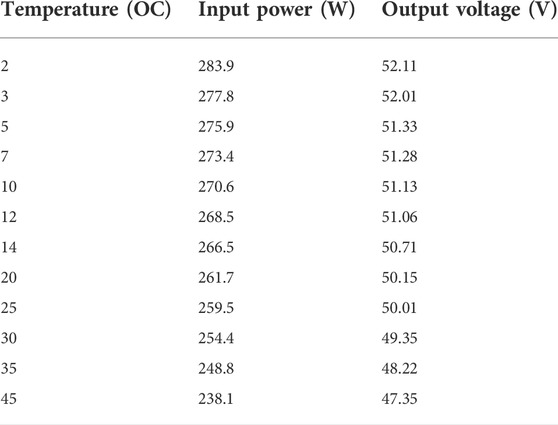
TABLE 4. Temperature, input PV power and output boost converter voltage readings.

FIGURE 9

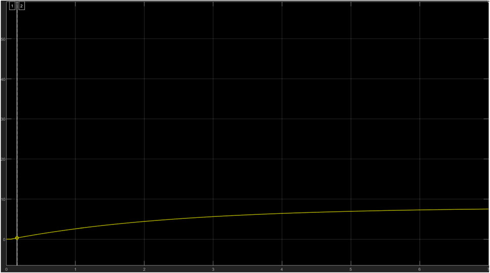
FIGURE 9. Output Voltage Waveform (7.965 V) at 100 irradiance.

FIGURE 10

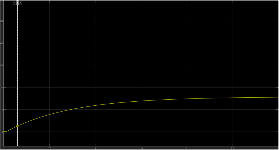
FIGURE 10. Output Voltage waveform (15.7 V) at 200 irradiance.

Further experimentation was done to show how the current and power characteristics vary under real-life conditions. [0 257 239 345,487 520,678 760,880 982,896 777,654 572,486 375,242 200,132], these values represent the irradiance readings extracted from an actual PV module which was embedded in SIMULINK within a simulation time of 2 s. Figures 11–22 show how temperature increases with a decrease in PV input power and with output boost converter voltage.

FIGURE 11

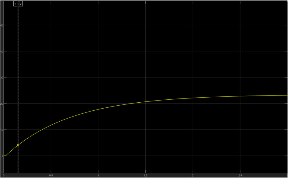
FIGURE 11. Output Voltage waveform (23.45 V) at 300 irradiance.

FIGURE 12

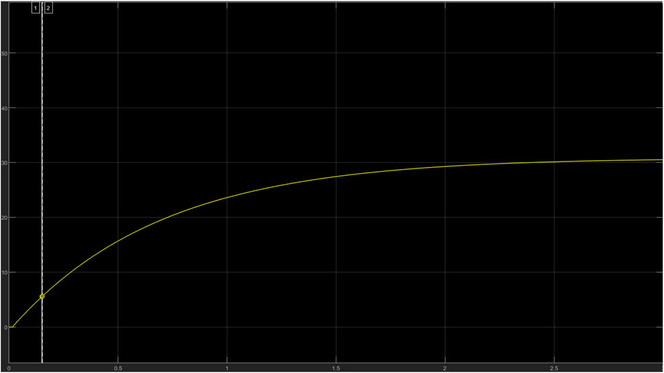
FIGURE 12. Output Voltage waveform (30.83 V) at 400 irradiance.

FIGURE 13

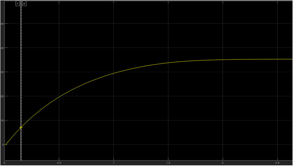
FIGURE 13. Output Voltage waveform (35.02) at 500 irradiance.

FIGURE 14

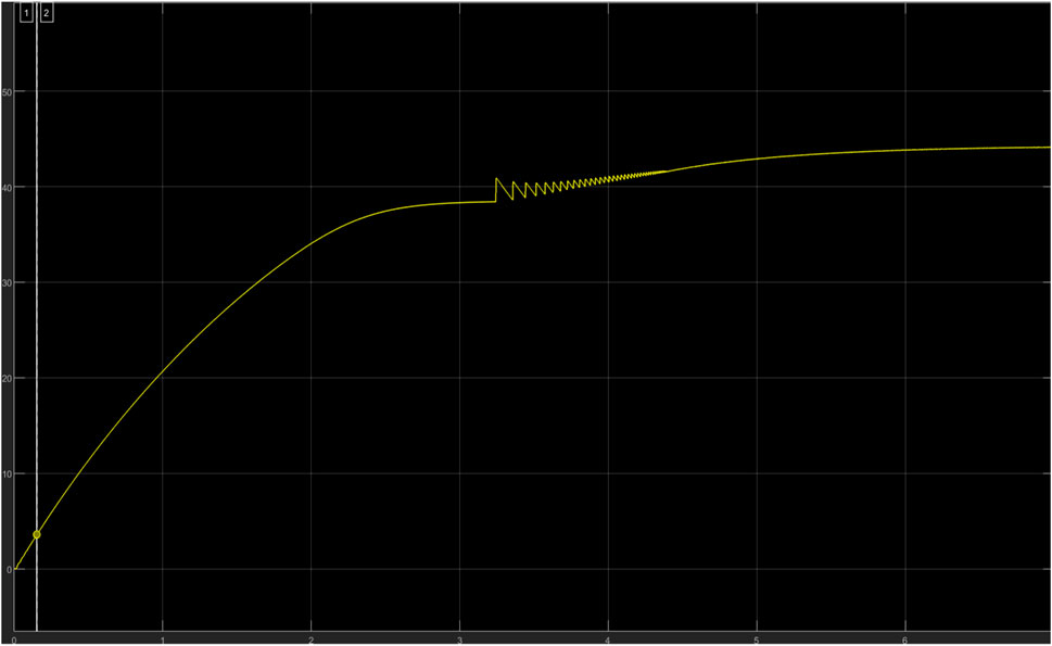
FIGURE 14. Output Voltage waveform (41.78 V) at 600 irradiance.

FIGURE 15

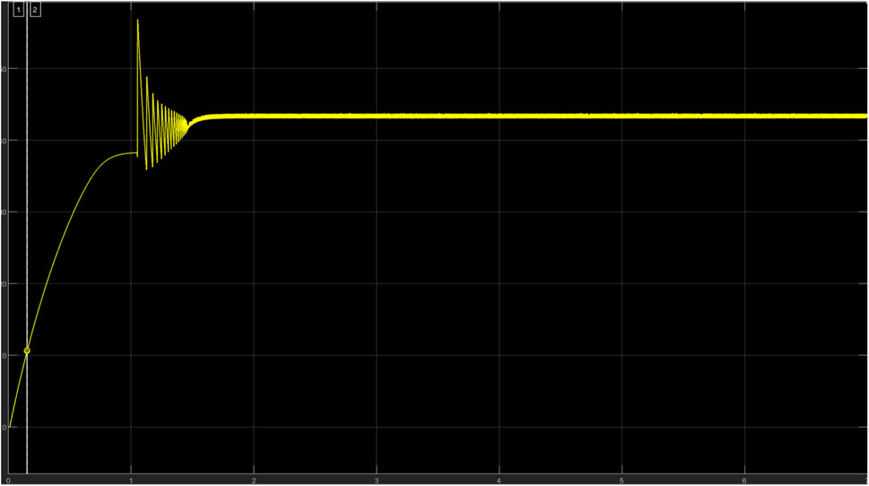
FIGURE 15. Output Voltage waveform (44.79 V) at 700 irradiance.

FIGURE 16

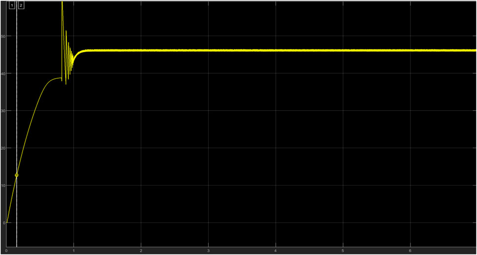
FIGURE 16. Output Voltage waveform (45.29 V) at 800 irradiance.

FIGURE 17

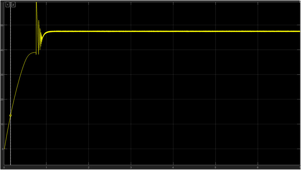
FIGURE 17. Output Voltage waveform (47.95 V) at 900 irradiance.

FIGURE 18

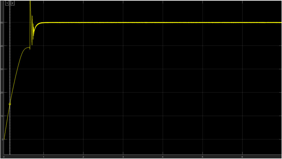
FIGURE 18. Output Voltage waveform (50.01 V) at 1000 irradiance.

FIGURE 19

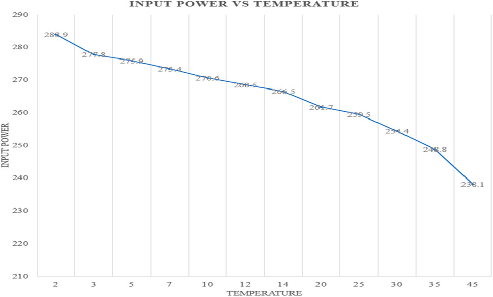
FIGURE 19. Input power for proposed PV Array against change in temperature.

FIGURE 20

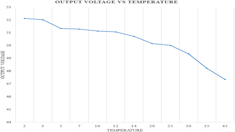
FIGURE 20. Output voltage of boost converter versus change in temperature.

FIGURE 21

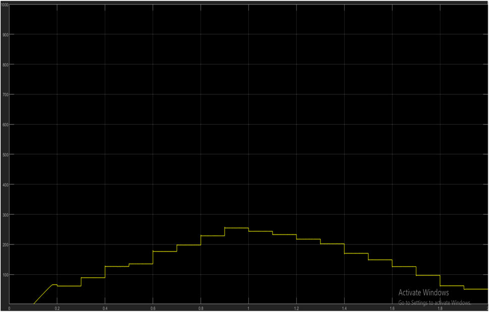
FIGURE 21. Power characteristics in response to unit step inputs of irradiance in MATLAB.

FIGURE 22

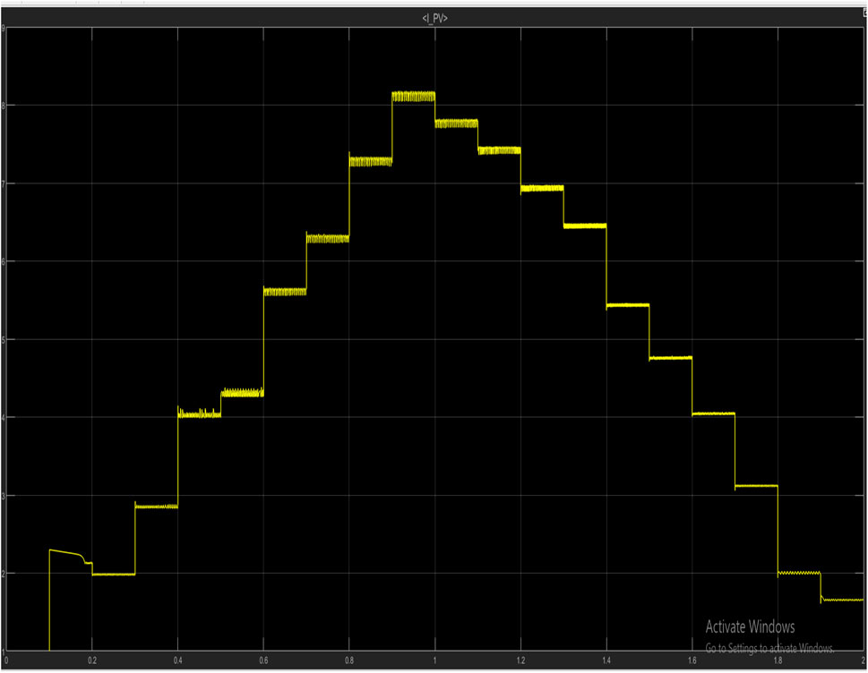
FIGURE 22. Current characteristics in response to various unit step irradiances in MATLAB.

4 Conclusion

In this study, a solar tracking model was developed using the P and O algorithm in conjunction with the PI controller. It can be seen that at different irradiance levels, particular maximum powerpoints are delivered to the load and or battery through a dc-dc chopper. This can also be seen with the variation of temperature on the PV array. The readings from the results obtained show that the use of perturb and observation algorithm coupled with the PI controller improves the efficiency of the PV array and the boost converter to a significant amount. Hence, this study has achieved improved and quality output power to charge battery and power loads from solar energy source.

Data availability statement

The original contributions presented in the study are included in the article/supplementary material, further inquiries can be directed to the corresponding author.

Author contributions

IS, Conceptualization, methodology, manuscript review and edit OI, Initial write-up, methodology TS, Initial write-up, Methodology, manuscript review and edit AA, manuscript review and edit JK, manuscript review and edit.

Acknowledgments

The authors wish to acknowledge the management of Covenant university for financial support and conducive environment provided for this study.

Conflict of interest

The authors declare that the research was conducted in the absence of any commercial or financial relationships that could be construed as a potential conflict of interest.

Publisher’s note

All claims expressed in this article are solely those of the authors and do not necessarily represent those of their affiliated organizations, or those of the publisher, the editors and the reviewers. Any product that may be evaluated in this article, or claim that may be made by its manufacturer, is not guaranteed or endorsed by the publisher.

References

Ahmed, J., and Salam, Z. (2018). An enhanced adaptive P&O MPPT for fast and efficient tracking under varying environmental conditions. IEEE Trans. Sustain. Energy 9, 1487–1496. doi:10.1109/tste.2018.2791968

CrossRef Full Text | Google Scholar

Anowar, M. H., and Roy, P. (2019). “A modified incremental conductance based photovoltaic MPPT charge controller,” in 2019 International Conference on Electrical, Computer and Communication Engineering (ECCE), 1–5.

CrossRef Full Text | Google Scholar

Anto, E. K., Asumadu, J. A., and Okyere, P. Y. (2016). PID-based P&O MPPT controller for offgrid solar PV systems using Ziegler-Nichols tuning method to step, ramp and impulse inputs. J. Multidiscip. Eng. Sci. Stud. (JMESS) 2.

Google Scholar

Argyrou, M. C., Christodoulides, P., and Kalogirou, S. A. (2018). “Modeling of a photovoltaic system with different MPPT techniques using MATLAB/Simulink,” in 2018 IEEE international energy conference (ENERGYCON), 1–6.

CrossRef Full Text | Google Scholar

Falayi, E., Usikalu, M., Omotosho, T., Ojoniyi, O., and Akinwumi, S. (2017). Impact of meteorological parameters over covenant university, Ota, Nigeria. J. Phys. Conf. Ser. 852, 012012. doi:10.1088/1742-6596/852/1/012012

CrossRef Full Text | Google Scholar

Han, Y., Luo, M., Zhao, X., Guerrero, J. M., and Xu, L. (2015). Comparative performance evaluation of orthogonal-signal-generators-based single-phase PLL algorithms—a survey. IEEE Trans. Power Electron. 31, 3932–3944. doi:10.1109/tpel.2015.2466631

CrossRef Full Text | Google Scholar

Hayat, M. B., Ali, D., Monyake, K. C., Alagha, L., and Ahmed, N. (2019). Solar energy—a look into power generation, challenges, and a solar‐powered future. Int. J. Energy Res. 43, 1049–1067. doi:10.1002/er.4252

CrossRef Full Text | Google Scholar

Jungbluth, N., Stucki, M., Flury, K., Frischknecht, R., and Büsser, S. (2012). Life cycle inventories of photovoltaics. Uster, Switzerland: ESU-Services Ltd., 250.

Google Scholar

Kim, D. S., Gabor, A., Yelunder, V., Upadhyaya, A., Meemongkolkiat, V., and Rohatgi, A. (2003). “String ribbon silicon solar cells with 17.8% efficiency,” in 3rd World Conference onPhotovoltaic Energy Conversion, 1293–1296.

Google Scholar

Kjær, S. B. (2012). Evaluation of the “hill Climbing&amp;#x201D; and the “incremental Conductance&amp;#x201D; maximum power point trackers for photovoltaic power systems. IEEE Trans. Energy Convers. 27, 922–929. doi:10.1109/tec.2012.2218816

CrossRef Full Text | Google Scholar

Koynov, S., Brandt, M. S., and Stutzmann, M. (2007). Black multi‐crystalline silicon solar cells. Phys. Stat. Sol. 1, R53–R55. doi:10.1002/pssr.200600064

CrossRef Full Text | Google Scholar

Kumar, N., Singh, B., and Panigrahi, B. K. (2019). ANOVA kernel Kalman filter for multi-objective grid integrated solar photovoltaic-distribution static compensator. IEEE Trans. Circuits Syst. I. 66, 4256–4264. doi:10.1109/tcsi.2019.2922405

CrossRef Full Text | Google Scholar

Kumar, N., Singh, B., and Panigrahi, B. K. (2019). PNKLMF-based neural network control and learning-based HC MPPT technique for multiobjective grid integrated solar PV based distributed generating system. IEEE Trans. Ind. Inf. 15, 3732–3742. doi:10.1109/tii.2019.2901516

CrossRef Full Text | Google Scholar

Mohapatra, A., Nayak, B., and Saiprakash, C. (2019). “Adaptive perturb & observe MPPT for PV system with experimental validation,” in 2019 IEEE International Conference on Sustainable Energy Technologies and Systems (ICSETS), 257–261.

Google Scholar

Nazir, F. U., Kumar, N., Pal, B. C., Singh, B., and Panigrahi, B. K. (2020). Enhanced sogi controller for weak grid integrated solar pv system. IEEE Trans. Energy Convers. 35, 1208–1217. doi:10.1109/tec.2020.2990866

CrossRef Full Text | Google Scholar

Osaretin, C., and Edeko, F. (2015). Design and implementation of a solar charge controller with variable output. Electr. Electron. Eng. 12, 40–50.

Google Scholar

Oyedepo, S. O., Anifowose, E. G., Obembe, E. O., and Khanmohamadi, S. (2021). “Energy-saving strategies on University campus buildings: Covenant University as case study,” in Energy Services fundamentals and financing (Elsevier), 131–154.

CrossRef Full Text | Google Scholar

Singh, B., Kumar, N., and Panigrahi, B. K. (2020). Steepest descent Laplacian regression based neural network approach for optimal operation of grid supportive solar PV generation. IEEE Trans. Circuits Syst. Ii. 68, 1947–1951. doi:10.1109/tcsii.2020.2967106

CrossRef Full Text | Google Scholar

Tan, R. H., Er, C. K., and Solanki, S. G. (2020). “Modeling of photovoltaic MPPT lead acid battery charge controller for standalone system Applications,” in E3s Web of conferences, 03005.

CrossRef Full Text | Google Scholar

Teja Manne, L. G. S., and Sy, F. (2018). Modeling of a photovoltaic array in MATLAB Simulink and maximum power point tracking using neural network. J. Electr. Electron. Syst. 7, 1–3. doi:10.4172/2332-0796.1000263

CrossRef Full Text | Google Scholar

Timilehin F, S., Ayobami, O., Ademola, A., and Gideon, A. (2019). Renewable energy towards a sustainable power supply in the Nigerian power Industry: Covenant university as a case study. Int. J. Mech. Eng. Technol. 10.

Google Scholar

Wolf, M., and Rauschenbach, H. (1963). Series resistance effects on solar cell measurements. Adv. energy Convers. 3, 455–479. doi:10.1016/0365-1789(63)90063-8

CrossRef Full Text | Google Scholar

Zeman, M., and Schropp, R. (1995). Amorphous silicon based solar cells and modules. Appl. Sol. ENERGY C/C GELIOTEKHNIKA 31, 22–29.

Google Scholar