An eco-technoeconomic analysis of hydrogen production using solid oxide electrolysis cells that accounts for long-term degradation

This paper presents an eco-technoeconomic analysis (eTEA) of hydrogen production via solid oxide electrolysis cells (SOECs) aimed at identifying the economically optimal size and operating trajectories for these cells. Notably, degradation effects were accounted by employing a data-driven degradation-based model previously developed by our group for the analysis of SOECs. This model enabled the identification of the optimal trajectories under which SOECs can be economically operated over extended periods of time, with reduced degradation rate. The findings indicated that the levelized cost of hydrogen (LCOH) produced by SOECs (ranging from 2.78 to 11.67 $/kg H₂) is higher compared to gray hydrogen generated via steam methane reforming (SMR) (varying from 1.03 to 2.16 $ per kg H₂), which is currently the dominant commercial process for large-scale hydrogen production. Additionally, SOECs generally had lower life cycle CO₂ emissions per kilogram of produced hydrogen (from 1.62 to 3.6 kg CO₂ per kg H₂) compared to SMR (10.72–15.86 kg CO₂ per kg H₂). However, SOEC life cycle CO₂ emissions are highly dependent on the CO₂ emissions produced by its power source, as SOECs powered by high-CO₂-emission sources can produce as much as 32.22 kg CO₂ per kg H₂. Finally, the findings of a sensitivity analysis indicated that the price of electricity has a greater influence on the LCOH than the capital cost.

1 Introduction

The widespread implementation of low-carbon electricity generation technologies such as nuclear, solar, and wind is a key step in the transition to a low-carbon future. However, the intermittent nature of solar and wind power limits their application compared to more reliable power sources, such as fossil-fuel-based power generators (Wang et al., 2010). On the other hand, nuclear plants can serve as baseload power generators, but this sometimes leads to power output exceeding demand. While this surplus power can be curtailed, doing so usually requires the payment of a penalty charge. Thus, the presence of large amounts of low-carbon power sources on the grid requires the use of storage systems to sequester surplus energy (Sgobbi et al., 2016). At present, batteries are the most common commercial energy storage systems in use, but their practical application is still somewhat limited due to their finite lifetime, use of limited rare earth materials, as well as environmental concerns relating to the carbon-intensive process used in their production and the water and air pollution caused by their disposal (Wang et al., 2010; Garraín et al., 2021). Electrolysers have shown considerable promise for energy storage, largely due to their higher energy storage density and lower environmental impact compared to lithium-ion batteries (Garraín et al., 2021). Hydrogen electrolysers are also key elements of the hydrogen economy (Parra et al., 2019). Electrolyser cells consume excess electricity from the grid to electrolyze water and produce hydrogen (Sgobbi et al., 2016), which is capable of storing high energy content per mass that can then be distributed and utilized for various applications (Züttel et al., 2010). For example, the produced hydrogen can be supplied to fuel cells during high-demand periods (day/year) to generate electricity to meet energy demands (Sgobbi et al., 2016), or it can be added to natural gas (NG) pipelines to lower the carbon intensity of NG (Parra et al., 2019). Furthermore, injecting hydrogen into the NG network eliminates the need for high-pressure hydrogen compressors, thereby reducing the system’s cost and energy consumption.

The ability to produce hydrogen via electrolysis is a major step towards enabling the hydrogen economy. Currently, steam methane reforming (SMR) is the most commonly used method for industrial-scale hydrogen production. The hydrogen generated through SMR, which has a low market price, is known as black or gray hydrogen due to its use of fossil fuels (coal and natural gas, respectively). Significant amounts of carbon dioxide are released during the SMR process. In contrast, electrolysers produce hydrogen without direct CO₂ emissions, but the source of the electricity used greatly impacts indirect CO₂ emissions. Hydrogen produced through electrolysis can be classified as green hydrogen if the electricity is exclusively derived from solar, wind, or geothermal energy (and biomass in some classifications), and pink hydrogen if it derives from nuclear energy. If mixed energy sources such as municipal power grids are used, life cycle CO₂ emissions can vary greatly from location to location and hour to hour. Thus, the carbon intensity of the electricity source plays an important role in the environmental performance of electrolysers (Muellerlanger et al., 2007).

The suitability of electrolysers for use in the hydrogen economy depends both on their economics and their CO₂ emissions per kg of hydrogen generated (Muellerlanger et al., 2007). Alkaline and proton-exchange membrane (PEM) electrolysers are among the most mature types of electrolysers and have been broadly used for hydrogen generation. Conversely, the large-scale commercialization of solid oxide electrolysis cells (SOECs) has yet to be achieved due to the high level of degradation often experienced by these cells. SOECs are efficient, as their high operating temperatures allow them to produce more hydrogen than low-temperature electrolysers per unit of electricity consumed (Sanz-Bermejo et al., 2015). While hydrogen production via alkaline and PEM electrolysers has been extensively studied (Yates et al., 2020; Bhandari and Shah, 2021; Gallardo et al., 2021), there remains a lack of research that examines the economic and environmental performance of SOECs while also considering their degradation. Indeed, a number of studies have investigated the economic optimization of SOECs, but none have employed a degradation-based model in doing so. For example, Seitz et al. performed an economic optimization of a solar-thermal-powered SOEC that had been integrated with thermal energy storage with the objective of minimizing the LCOH (Seitz et al., 2017). They compared their results with the LCOH of a standalone SOEC and found that the addition of thermal energy storage decreased the LCOH from 0.16 to 0.11 EUR/kWh H₂. However, Seitz et al.’s analysis completely ignored the influence of electrolysis cell degradation. Elsewhere, Mastropasqua et al. proposed an SOEC system that was integrated with a parabolic dish solar field to enable the generation of 150 kg H₂ per day (Mastropasqua et al., 2020). Even though Mastropasqua et al.’s models used thermodynamic equations to quantify the inevitable overpotentials of the electrolysis cells, they did not account for the degradation that occurs due to the system reactions. In another study, Lahdemaki used Aspen Plus to develop a black box model for an SOEC system sized to generate enough hydrogen to enable the production of 6,000 t of synthetic natural gas (in this paper, t = tonne = 1,000 kg). A number of simplifying assumptions were made both in their model and in their optimization problem. For instance, it was assumed that SOECs degrade at a constant rate of 0.3% per 1,000 h, and that 16,169 m² of cells are required. To calculate the degradation rate, it was assumed that the system’s power consumption increases by almost 10% after 40,000 h of use.

The current paper presents an eco-technoeconomic analysis (eTEA) of SOECs aimed at identifying the optimal operating trajectories for economical hydrogen production. Unlike previous works, we use a data-driven model developed in a prior work (Naeini et al., 2022) for SOEC performance degradation (Hoerlein et al., 2018). The developed model, which will be described in the next section, describes how SOEC performance changes over time under specific operating conditions. To the best of the authors’ knowledge, this is the first eTEA of SOECs to employ a degradation-based model. This is significant, as the incorporation of a degradation-based model will yield findings that are more accurate and reliable compared to those of other studies in the open literature, which have either ignored or underrated SOEC degradation. The results of this work will allow us to determine whether adjusting the operating parameters can make SOECs economically competitive with mature hydrogen-production technologies, despite their degradation and high capital cost. Since capital costs associated with SOECs can vary significantly with manufacturing volume and electricity rates vary between grids and time (i.e., peak vs. off-peak), a sensitivity analysis is conducted to determine the extent to which these factors influence the cost of hydrogen production. The results of such sensitivity analyses are critical in determining whether SOECs are an economically viable option for a particular region. Furthermore, CO₂ emissions per kg of hydrogen generated is another key factor that must be considered when selecting the best technology for use in the hydrogen economy. As such, CO₂ emissions associated with SOEC manufacturing and electricity generation from various sources are calculated to determine whether SOECs are suitable for use in the hydrogen economy, and how its suitability is affected by grid emissions. Finally, the cost of CO₂ avoided (CCA) is also computed to provide a good metric for comparing SOECs with other hydrogen-production processes, both in terms of economic and environmental performance.

2 Background

2.1 Data-driven model for long-term SOEC performance

SOECs have the same components and structure as solid oxide fuel cells (SOFCs). SOFCs convert the chemical energy from a fuel source to electricity through electrochemical reactions between fuel and oxygen; in contrast, electrical charge moves in the opposite direction in SOECS, electrolyzing steam through endothermic electrochemical reactions (Klotz et al., 2014). In a previous study, we developed a detailed model that captures how six mechanisms that govern SOFC degradation impact its long-term performance (Naeini et al., 2021a). It is important to note that, since the reactants and electrochemical reactions in SOFCs and SOECs are different, the dominant degradation mechanisms will also be different. Therefore, the SOFC degradation model is unable to describe degradation in SOECs. Due to a lack of adequate openly available information about the various degradation reactions in SOECs, it is not yet possible to construct a first-principles model for SOECs. Consequently, we constructed a data-driven model in our prior work using Hoerlein et al.’s experimental results, which provide data for identical SOECs under various temperatures, current densities, and fuel humidity percentages over 1,000 h of operation (Hoerlein et al., 2018; Naeini et al., 2022). The findings of Hoerlein et al.’s studies have shown that temperature, current density, and fuel gas humidity have the highest impacts on SOEC degradation. As such in (Hoerlein et al., 2018) they only investigated and showed the impacts of these parameters on degradation of the cells. In their work, Hoerlein et al. took increases in a cell’s ohmic resistance as a key indicator of the degradation. Changes in the SOEC’s ohmic resistance over time can be used to quantify the degradation of SOECs. Several studies have shown that the ohmic overpotential, which can be calculated by Ohm’s law, is the main and the most substantial contributor to the SOEC overpotential (Ni, 2010; Zhang et al., 2013; Guan et al., 2014; Mendoza et al., 2020). The rate of hydrogen production by SOECs has a linear correlation with current density (Eq. 1); this means that a constant current density leads to a constant hydrogen production rate in SOEC.

${\dot{n}}_{H_{\mathit{2}}}=\frac{i}{n_e\mathrm{F}}(1)$

In this equation ${\dot{n}}_{H_{\mathit{2}}}$ is the rate of hydrogen production by SOEC, $i$, $n$, and $\mathrm{F}$ are the current density, moles of electrons transferred in the electrolysis reactions, and Faraday constant, respectively. The energy needed for production of a constant amount of hydrogen by the SOEC increases with its ohmic resistance and degradation (Eq. 2).

$P=R{i}^{\mathit{2}}=Vi(2)$

where $P$, $V$, and $R$ are the SOEC’s power, voltage, and ohmic resistance, respectively. The amount of resistance increase over time is a function of the SOEC’s operating parameters. In our prior work, we used the data from Hoerlein et al.’s experiments (Figure 1) to build a model that predicts temporal change of resistance with respect to current density, temperature, and the fuel gas molar humidity. (Naeini et al., 2022) This model quantifies degradation of SOEC as a function of the operating conditions.

FIGURE 1

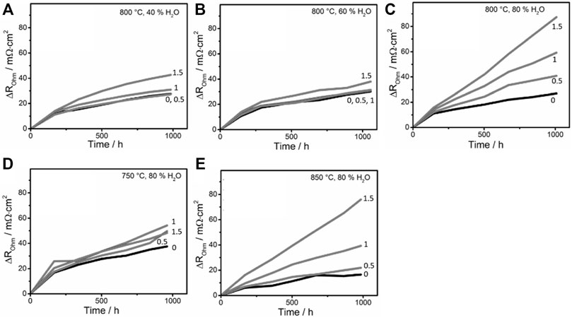
FIGURE 1. Temporal change of ohmic resistance of SOECs at different current densities from 0 to 1.5 A/cm² and (A) 800°C and 40% fuel humidity, (B) 800°C and 60% fuel humidity, (C) 800°C and 80% fuel humidity, (D) 750°C and 80% fuel humidity, and (E) 850°C and 80% fuel humidity measured by Hoerlein et al. (2018) The y-axis, $∆R_{ohm}$, is the ohmic resistance increase from the initial ohmic resistance of SOECs. Figure reused with permission from (Naeini et al., 2022).

Hoerlein et al. ensured that a wide range of operating parameters were investigated in their study by varying the temperature from 750 to 850°C, the current density from 0 to 1.5 A/m², and the fuel gas molar humidity from 40% to 80% (Hoerlein et al., 2018). The tested SOECs were in transition period over the first 200 h of use and showed an unstable trend that cannot be modelled. This unstable behavior was also observed previously by other research groups (Sohal, 2009; Hubert, 2018). It is worth noting that, even though the degradation trend in the transition period is not reproducible, the value of cumulative degradation at 200 h can be modelled with respect to the operating parameters. As such, we removed the transition period data and used the remaining data to generate the model. In our prior work, we employed Automated Learning of Algebraic Models (ALAMO) to identify an algebraic model from the training dataset (Naeini et al., 2022).

2.1.1 The linear model from 200h to 2500h

Eq. 3 is the linear model generated by ALAMO for the time evolution of SOEC performance degradation.

$R_{t^{\prime }}=R_{\mathrm{0}}+\mathrm{0.019}TH+\mathrm{7.290}Hi+\mathrm{0.033}H{t}^{\prime }+\mathrm{0.017}i{t}^{\prime }(3)$

In this equation $t^{\prime }$ represents the time since the 200 h transition period has completed (h), $R_{t^{\prime }}$ and $R_{\mathit{0}}$ are the SOEC’s ohmic resistance (mΩ.cm²) at times $t^{\prime }$ and 0 h (the virginal state), respectively, $T$ is the cell’s operating temperature (°C), $H$ is the mole fraction of water in the fuel gas known as fuel gas humidity, and $i$ is the current density (A/cm²). Time-independent terms show the accumulated increase in resistance over the transition period, while time-dependent terms show time variation of ohmic resistance after 200 h. When the supplied current density and fuel gas humidity are constant, the model shows linear growth in resistance over time. Even though this linear trend was observed in several experimental studies on SOECs, it should be noted that all of these studies tested SOECs for 2,500 h or less (Hauch et al., 2006; Trofimenko et al., 2017; Hubert, 2018).

2.1.2 Validation of the linear model (out to 2500h)

The linear model was compared against Tietz et al.’s experimental data—which was not used in developing the model—for validation purposes (Figure 2), with the results indicating that the linear model had good ability to predict SOEC degradation over the first 2,500 h (Tietz et al., 2013). However, Tietz et al.’s data, which was collected over almost 7,600 h of SOEC operation, indicated that the degradation rate diminishes after 2,500 h; thus, the linear model deviated from Tietz et al.’s data after this time. It should be noted that most experiments that show linear degradation rates for SOECs, such as (Hauch et al., 2006; Trofimenko et al., 2017; Hubert, 2018), are not performed for long enough to encounter the deviation from linear trend at around 2500h.

FIGURE 2

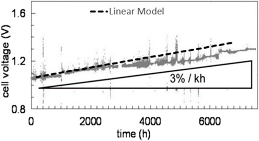
FIGURE 2. Results of the simulation of performance degradation in SOEC using our linear model compared to experimental data from (Tietz et al., 2013). Our linear model is drawn as a dashed line on a modified version of the original figure reproduced from that work. Figure reused with permission from (Naeini et al., 2022).

2.1.3 Sublinear model

The model was subsequently modified into a sublinear model by introducing an exponent term to the time component ($t^{\prime }$). The value of the power term was calculated by fitting it to Tietz et al.’s experimental data. The modified model is expressed as follows:

$R_{t^{\prime }}=R_0+0.019TH+7.290Hi+\left(0.033H+0.017i\right){\left(t^{\prime }\right)}^{0.97}(4)$

Comparison of Tietz et al.’s experimental data, the linear model, and sublinear model (Figure 3) indicates that the linear model is almost as good as the sublinear model for prediction of SOEC’s short-term performance. But as can be seen the modified model is substantially better for simulation of the long-term performance of SOECs. Even though this model only accounts for the ohmic overpotential, the model showed a very good agreement with the validation data. Because as it was mentioned above concentration and activation overpotentials have small contributions to the overall overpotential of the cells comparing to the ohmic overpotential.

FIGURE 3

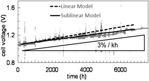
FIGURE 3. Results of the simulation of long-term performance degradation in SOEC using the linear and sublinear models compared to experimental data from (Tietz et al., 2013). Our linear and sublinear models are drawn as dashed and solid lines, respectively, on a modified version of original figure. Figure reused with permission from (Naeini et al., 2022).

Even though there are not many studies in the open literature that run experiments long enough to observe the sublinear trend of degradation rate, this trend makes sense, since actual SOEC systems are operated for several years. If SOECs were degrading linearly with time at the rates suggested by the linear model, the magnitude of degradation in the long-term would be significantly higher than what actual SOECs undergo, and their lifetimes would be substantially shorter. As such it is important to use the modified model for simulation of long-term operations as it will have considerable impacts on the design and operation of large SOEC systems.

We note that this model can be further modified in the future to be more representative of degradation of SOEC stacks. Currently, there is a lack of sufficient long-term experimental data on stacks of SOEC under different operating conditions which is due to the high cost and long time of these experiments.

2.2 Model for steady-state SOEC operation

The developed data-driven model projects an increase in SOEC resistance as a result of degradation. As can be seen in Eq. 4, when quantifying the time evolution of resistance under specific operating conditions, it is necessary to know the cells’ initial resistance under those conditions. The first-principles model in the literature that is commonly used to describe the steady-state performance of SOECs is applied in this work to calculate the voltage of the SOECs prior to degradation. For a more detailed description of this model, the reader is referred to (Ni et al., 2007; Habibollahzade et al., 2019). By combining the first-principles model with Eq. 4 and Ohm’s law (Eq. 5), it is possible to quantify the SOEC’s performance at each time point.

$V=iR(5)$

$V_{t^{\prime }}=V_0+i\ast \left[0.019TH+7.290Hi+\left(0.033H+0.017i\right){\left(t^{\prime }\right)}^{0.97}\right](6)$

Where $V_{\mathit{0}}$ is the voltage of the cells at 0 h, which is obtained via the first-principles model (V). Eq. 6 is applied in the optimization problem to find the operating trajectories best suited for producing hydrogen at the minimum cost. The details of the optimization problem will be discussed in the next section.

3 Methodology: Eco-technoeconomic analysis of SOECs

The aforementioned model (Eq. 6) was employed in an eco-technoeconomic analysis (eTEA) to determine the optimal trajectories for generating hydrogen via SOECs economically, while accounting for cell degradation. Specifically, this eTEA aimed to minimize the levelized cost of hydrogen (LCOH) generated by SOECs during their operational lifespan. Although LCOH has been computed for SOEC systems in a number of prior studies (Seitz et al., 2017; Mastropasqua et al., 2020; Hauth et al., 2021), we are unaware of any previous eTEA that accounts for SOEC degradation. This factor is critical, as the rate of SOEC degradation which changes in response to the operating conditions, can substantially impact the lifetime and economic efficiency of SOECs. Thus, the present research makes an important contribution to the literature, as it provides a realistic answer to the long-standing question: “can SOECs, with their existing design and structure, become economically competitive with current hydrogen-production technologies?”

Due to the lack of a definitive definition for the lifetime of SOECs or SOFCs, we include cell lifetime as a parameter in this eTEA’s optimization problem, which outlines our planned cell-replacement schedule (Naeini et al., 2021b). The optimization problem contains a number of assumptions. First, it is assumed that the problem is solved over a 20-year project lifetime, and that the SOECs have a lifetime of $L$ years. SOECs are decommissioned after $L$ years of operation and replaced with identical new cells with the same active membrane area and operating conditions. Second, it is assumed that the lifetime parameter ($L$) ranges from 1 to 14 years, and that the problem is solved for each $L$ value separately (Naeini et al., 2021b). SOFCs and SOECs can experience catastrophic failure during long-term operations; the duration of operation prior to catastrophic failure depends on the cell’s operating conditions and cannot be predicted by existing degradation models. In a recent experimental study on SOECs, researchers were able to assess the performance of SOECs for 14 years prior to catastrophic failure (Hauch et al., 2020). To the best of our knowledge, this is the longest time reported for the operation of solid oxide cells before catastrophic failure occurred. As such, we took 14 years as the maximum replacement time, and we solved the problem for replacement periods of 1–14 years. These are the same as the assumptions used in our previous TEA of SOFCs (Naeini et al., 2021b).

We implemented and solved the economic hydrogen-production optimization problem in general algebraic modeling system (GAMS). The objective in doing so was to determine the optimal active membrane area for use in SOECs and their optimal operating trajectories for generating hydrogen with a minimal LCOH. We also used CONOPT solver, which is well-suited to solving large non-linear problems (NLP) quickly, and is particularly suitable in situations where a feasible solution cannot be easily achieved (The CONOPT Algorithm, 1999). A description of the system and a detailed mathematical explanation of the problem is provided below for SOECs with $L$ years replacement plan.

$\underset{T_j,H,i_j,A_m,X_j}{\mathit{min}}LCOH(7)$

A number of equations have been used to calculate $LCOH$ that are slightly different from one another. In this study, we selected Eq. 8 to calculate $LCOH$ because it accounts for the time value of money and it is the equation most commonly used in the literature (Seitz et al., 2017; Mohammadi and Mehrpooya, 2018; Yadav and Banerjee, 2018).

$LCOH=\frac{CRF\times CC+OC+EC}{n_{H_2,del,tot}\times {HHV}_{H_2}\times 0.28\times {10}^{-3}\frac{kWh}{kJ}}(8)$

In this equation: $LCOH$ is calculated in $/kWh_HHV; $CC$, $OC$, and $EC$ are the total capital costs, non-electricity operating and maintenance costs, and electricity costs ($), respectively; $n_{H_{\mathit{2}},del,tot}$ is the total moles of hydrogen delivered by SOECs over the 20-year life of the plant (mol); ${\mathrm{H}\mathrm{H}\mathrm{V}}_{{\mathrm{H}}_2}$ is the higher heating value of hydrogen (285.8 kJ/mol); and $\mathrm{C}\mathrm{R}\mathrm{F}$ is the capital recovery factor. The CRF is calculated as follows:

$CRF=\frac{r\times {\left(\mathrm{1}+r\right)}^N}{{\left(\mathrm{1}+r\right)}^N-\mathrm{1}}(9)$

where $r$ is the discount rate, which is set at a value of 10%, and $N$ is the plant’s lifetime, which is 20 years in this work.

Subscript $j$ in the decision variables (Eq. 7) is the time-step indicator. Each time step in this optimization problem is 5 days (120 h), meaning that there are 73 time steps every year. Decision variables such as temperature, current density, and mole gas recycled per mole produced ($X$) are functions of time and are held constant for each time step. In contrast, fuel gas humidity is not time dependent.

Equations 10–12 show the lower and upper bounds for temperature, current density, and fuel gas humidity in the optimization problem. These are the acceptable ranges found for the operation of SOECs in the open literature (Wang et al., 2010; Sanz-Bermejo et al., 2015; Hoerlein et al., 2018). The fuel gas should contain some hydrogen to make a reducing environment and prevent fuel electrode oxidation. Usually, a minimum content of 20% hydrogen is required for this purpose (Kim et al., 2015; Hoerlein et al., 2018).

$923\le T_j\le 1073\left(K\right)(10)$

$100\le i_j\le 18000\left(A/m^2\right)(11)$

$0.4\le H\le 0.8(12)$

As can be seen in Eq. 4, the resistance of the cells, and thus their degradation, is highly affected by the current density. Additionally, the hydrogen molar production rate varies in response to changes in the current density. Thus, sudden or large variations in the current density should be avoided to ensure safe and realistic operation. As noted above, current density is held fixed for each time step, and Eq. 13 is then used to ensure that it changes less than $\pm$10% for the next time step.

$0.9\times i_{j-1}\le i_j\le 1.1\times i_{j-1}(13)$

Temperature also significantly impacts the degradation and lifetime of SOECs. Abrupt changes to the cell’s temperature or extensive temperature gradients along the cells should be avoided, as they may result in catastrophic failure. Due to a lack of information, the proposed model of SOEC degradation cannot predict when catastrophic failure will happen under different operating conditions. As such, we employ conservative constraints to encourage safe long-term SOEC operation. The temperature of the cells is constant for each time step and constrained to vary less than $\pm$1% for the next time step via Eq. 14.

$0.99\times T_{j-1}\le T_j\le 1.01\times T_{j-1}(14)$

The following constraints are added to limit the temperature gradient between the inlet and outlet of the cells to $\pm$1% of the cells’ temperature.

$0.99\times T_j\le T_{in,j}\le 1.01\times T_j(15)$

$0.99\times T_j\le T_{out,j}\le 1.01\times T_j(16)$

The voltage of the cells is calculated via Eq. 6. Normally, SOECs have a voltage of between 0.6 and 1.8 V (Mogensen et al., 2019).

$\mathrm{0.6}\le V_j\le \mathrm{1.8}$ (17)

The mass balance of the system is provided in the following equations. As it was mentioned in Section 2 the hydrogen molar production rate has a linear correlation with the current supplied to the cells and Eq. 1 can be rewritten as:

${\dot{n}}_{H_{\mathrm{2}p,j}}=\frac{A_m\times i_j\times \mathrm{3600}\frac{s}{h}}{\mathrm{2}\times F}(18)$

where ${\dot{n}}_{H_{\mathit{2},p,j}}$ is the molar production rate of hydrogen in (mol/h) and $F$ is the Faraday constant. The steam molar consumption rate is equal to the production rate of hydrogen, as shown in Eq. 19.

${\dot{n}}_{H_{\mathrm{2}}{O}_{c,j}}={\dot{n}}_{H_{\mathrm{2},p,j}}(19)$

SOECs do not utilize all of the steam they are supplied with. The molar rate at which steam is fed into the cells can be calculated as follows via Eq. 20.

${\dot{n}}_{H_{\mathrm{2}}{O}_{in,j}}=\frac{{\dot{n}}_{H_{\mathrm{2}}{O}_{c,j}}}{SU}(20)$

In this equation, $SU$ is steam utilization, which is assumed to be 80% in this study. The inlet stream to SOECs consists of steam and some hydrogen. If the fuel gas humidity and steam supply molar rate are known, then the molar rates of total fuel gas supply and the hydrogen content of the fuel gas can be determined using Eqs 21, 22, respectively.

${\dot{n}}_{{TOT}_{in,j}}=\frac{{\dot{n}}_{H_{\mathrm{2}}{O}_{in,j}}}{H}(21)$

${\dot{n}}_{H_{\mathrm{2}in,j}}=\left(\mathrm{1}-H\right)\times {\dot{n}}_{{TOT}_{in,j}}(22)$

where ${\dot{n}}_{{TOT}_{in,j}}$ and ${\dot{n}}_{H_{\mathit{2}in,j}}$ are the molar rates of the total inlet fuel gas and its hydrogen content, respectively. The cathode outlet contains hydrogen and some unreacted steam. Next, the molar rates of the gases in the cathode outlet can be determined via Eqs 23, 24.

${\dot{n}}_{H_{\mathrm{2}out,j}}={\dot{n}}_{H_{\mathrm{2}in,j}}+{\dot{n}}_{H_{\mathrm{2}p,j}}(23)$

${\dot{n}}_{H_{\mathrm{2}}{O}_{out,j}}={\dot{n}}_{H_{\mathrm{2}}{O}_{in,j}}-{\dot{n}}_{H_{\mathrm{2}}{O}_{c,j}}(24)$

Pure oxygen is produced by the electrolysis reaction and leaves the anode at the following rate,

${\dot{n}}_{O_{\mathrm{2}out,j}}=\mathrm{0.5}\times {\dot{n}}_{H_{\mathrm{2}p,j}}(25)$

A part of the cathode outlet can be recycled and used in the next time periods.

${\dot{n}}_{H_{\mathit{2}}{O}_{in,j}}={\dot{n}}_{H_{\mathrm{2}}{O}_{f,j}}+X_j\times {\dot{n}}_{H_{\mathrm{2}}{O}_{out,j-\mathrm{1}}}(26)$

${\dot{n}}_{H_{\mathrm{2}in,j}}=X_j\times {\dot{n}}_{H_{\mathrm{2}out,j-\mathrm{1}}}(27)$

In Eq. 26, ${\dot{n}}_{H_{\mathit{2}}{\mathrm{O}}_{\mathrm{f},j}}$ is the molar rate of fresh water to be supplied to the cells and $X_j$ is the mole recycled per total mole produced.

Finally, the rate of hydrogen delivered by the SOEC system in the $j$th time step can be determined by,

${\dot{n}}_{H_{\mathrm{2}del,j}}=\left({\mathrm{1}-X}_{j+\mathrm{1}}\right)\times {\dot{n}}_{H_{\mathrm{2}out,j}}(28)$

While the total moles of hydrogen delivered by SOECs over the project’s 20-year lifetime is defined as,

$n_{H_2,del,tot}=\frac{N}{L}\times {\displaystyle \sum }_{j=1}^{L\times 73}120\left(h\right)\times {\dot{n}}_{H_{2del,j}}(29)$

where $n_{H_{\mathit{2}},del,tot}$ is the moles of hydrogen delivered by SOECs over 20 years and $L$ is the replacement schedule or lifetime of the cells (years). To ensure a good comparison between SOECs with different replacement schedules, we restrict SOEC production to an average of 550 MW of hydrogen (based on ${\mathrm{H}\mathrm{H}\mathrm{V}}_{{\mathrm{H}}_2}$) over their lifetime.

$\frac{{\displaystyle \sum }_{j=1}^{L\times 73}{\dot{n}}_{H_{2del,j}}\times {HHV}_{H_2}}{L\times 73}\times 0.28\times {10}^{-6}\frac{MW}{kJ/h}=550\left(MW\right)(30)$

The energy balance of the system can be described by,

$P_{DC,j}+E_{in,j}-E_{out,j}=0(31)$

where $P_{\mathrm{D}\mathrm{C},j}$ is the DC power supplied to the SOECs in the $j$th time step, and $E_{in,j}$ and $E_{out,j}$ are the inlet and outlet enthalpy flows (MW), respectively. $P_{\mathrm{D}\mathrm{C},j}$ is computed via Eq. 32.

$P_{DC,j}=i_j\times V_j\times A_m\times {\mathrm{10}}^{-\mathrm{6}}\frac{MW}{W}(32)$

To provide $P_{\mathrm{D}\mathrm{C},j}$ (MW), AC power is drawn from the grid and converted to DC through an AC/DC inverter, which is assumed to have a 96.5% efficiency (Naeini et al., 2021b). As such, AC power supply in the $j$th time step can be computed as follows:

$P_{AC,j}=\frac{P_{DC,j}}{96.5\%}(33)$

$Q_{in,j}=\left[{\dot{n}}_{H_{2in,j}}{C}_{p{H}_2}\left(T_{in,j}-T_1\right)+{\dot{n}}_{H_2{O}_{in,j}}{C}_{p{H}_{2}O,g}\left(T_{in,j}-T_2\right)+{\dot{n}}_{H_2{O}_{in,j}}{L}_{v{H}_{2}O}+{\dot{n}}_{H_2{O}_{in,j}}{C}_{p{H}_{2}O,l}\left(T_2-T_1\right)\right]\times 2.8\times {10}^{-10}\frac{MW}{J/h}(34)$

$\begin{array}{c}{Q}_{out,j}=[{\dot{n}}_{H_{2out,j}}{C}_{p{H}_2}\left(T_{out,j}-T_1\right)+{\dot{n}}_{H_2{O}_{out,j}}{C}_{p{H}_{2}O,g}\left(T_{out,j}-T_2\right)\\ +{\dot{n}}_{H_2{O}_{out,j}}{L}_{v{H}_{2}O}+{\dot{n}}_{H_2{O}_{out,j}}{C}_{p{H}_{2}O,l}\left(T_2-T_1\right)\\ +{\dot{n}}_{O_{2out,j}}{C}_{p{O}_2}\left(T_{out,j}-T_1\right)]\times 2.8\times {10}^{-10}\frac{MW}{J/h}\end{array}(35)$

In the above equations, $C_{pk}$refers to the molar heat capacity of species, $k$ (J/molK), which varies with temperature according to the model found in (Petipas et al., 2013). $T_{\mathit{1}}$ is the reference temperature (298 K), $T_{\mathit{2}}$ is the evaporation temperature of water at 4 bar (416 K)—the assumed operation pressure for SOECs—and $L_{v{H}_{\mathit{2}}O}$ is the latent heat of vaporization of water (J/mol).

All costs in this work are given in 2016 U.S. dollars. Unlike mature technologies, the capital costs of SOECs depend on its commercialization status and production volume. Myrdal et al. consulted number of references and calculated capital costs of SOEC systems for various production volumes at different times (Mýrdal et al., 2016). To reduce error, we used the SOEC system costs obtained by Myrdal et al. between 2015 and 2017 through consultations with manufacturers, rather than their predicted costs for after 2017. Myrdal et al. catalogued the costs of SOECs with production volumes ranging from 1,250 to 250,000 m²/year, but we use the costs of SOECs with a production volume of 125,000 m²/year in this eTEA. SOECs produced between 2015 and 2017 at rate of 125,000 m²/year cost 0.24 $/cm², which includes the ab factory and turnkey costs. Ab factory costs consists of the costs of the equipment and a 50% mark up. The balance-of-plant (BoP) items in an SOEC system normally include heat exchangers, a compressor, pumps, piping and connections, and electronics. The capital costs of BoP items, excluding the compressor, were 0.596 $/cm² of active membrane area installed. This includes costs of heat exchangers, AC/DC inverter, pumps, and separator (flash drum). The present study does not include a detailed model for BoP components. As BoP designs will differ from case to case, it was best to restrict the boundary to the present system in order to have a more generalized result. In this study, the produced hydrogen has a high quality with ∼97% purity and is used outside of the system’s boundaries. As such, a high-pressure hydrogen compressor and storage are not used in this work. An outline of the system can be seen in Figure 4.

FIGURE 4

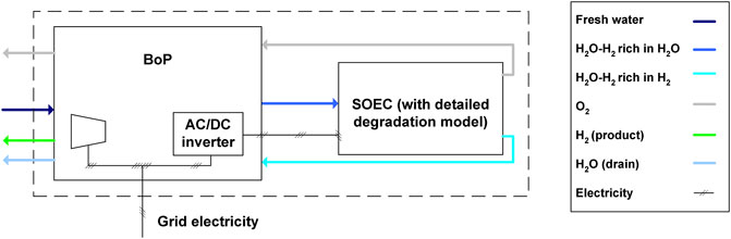
FIGURE 4. An outline of the SOEC system.

In a standalone SOEC system, fresh water is evaporated and mixed with hydrogen before being fed into the SOECs. The thermal energy required to pre-heat the fuel gas stream is provided by the anode and cathode outlet streams, which leave the cells at high temperature. Heat transfer takes place through multiple heat exchangers, and the hydrogen for the fuel gas mixture is recycled from the cathode outlet. The cathode outlet pressure slightly drops in the heat exchanger before part of it is recycled and mixed with the fresh water. The recycled stream is passed through a compressor to raise its pressure to 4 bar. The compressor is an expensive component in the BoP, its size depends on the value of $X_j$, and it can substantially increase system costs. Therefore, the capital cost of the compressor is calculated separately as

${CC}_{comp.}={UC}_{comp.}\times \frac{{\displaystyle \sum }_{j=1}^{L\times 73}{comp.work}_j}{L\times 8760}(36)$

where ${CC}_{\mathrm{c}\mathrm{o}\mathrm{m}\mathrm{p}.}$ is the capital cost of the compressor ($), ${\mathrm{U}\mathrm{C}}_{\mathrm{c}\mathrm{o}\mathrm{m}\mathrm{p}.}$ is the unit cost of the compressor and takes the value of 24.455 $/kW, and ${comp.work}_j$ is the compressor work in kWh, which is defined as follows. (Mýrdal et al., 2016; NASA, 2021)

${comp.work}_j=CW\times \left(X_j\times {\dot{n}}_{H_{2out,j}}+X_j\times {\dot{n}}_{H_2{O}_{out,j}}\right)\times 120\times {10}^{-3}(37)$

In the above equation, $CW$ is the compressor work per mole of gas (kWh/kmol), which is computed via Eq. 38, (NASA, 2021)

$CW=\frac{c_p\times T_{comp.in}}{{\eta }_{comp.}}\left({CPR}^{\frac{\gamma -1}{\gamma }}-1\right)(38)$

where $c_p$ is the specific heat capacity of the gas (kWh/kmolK); $T_{comp.in}$ is the temperature of the gas at the compressor inlet and is assumed to be 453 K; ${\eta }_{comp.}$ is the compressor efficiency, which is assumed to be 82%; $CPR$ is the compressor pressure ratio; and $\gamma$ is the specific heat ratio.

$CPR=\frac{{\mathit{Pr}}_{comp.out}}{{\mathit{Pr}}_{comp.in}}(39)$

In Eq. 39, ${\mathit{Pr}}_{comp.in}$ and ${\mathit{Pr}}_{comp.out}$ are the pressure of the gas at the inlet and outlet of the compressor, which are 3.9 and 4 bar in this study, respectively.

The capital costs of SOEC and the remaining of BoP components are given in Eqs 40, 41.

${CC}_{SOEC}=\frac{N}{L}\times {UC}_{SOEC}\times A_m\times {10}^4(40)$

${CC}_{BoP}={UC}_{BoP}\times A_m\times {10}^4(41)$

In the above equations, ${CC}_{\mathrm{S}\mathrm{O}\mathrm{E}\mathrm{C}}$ and ${CC}_{\mathrm{B}\mathrm{o}\mathrm{P}}$ are the capital costs of the SOEC and BoP items ($), respectively, and ${\mathrm{U}\mathrm{C}}_{\mathrm{S}\mathrm{O}\mathrm{E}\mathrm{C}}$ and ${\mathrm{U}\mathrm{C}}_{\mathrm{B}\mathrm{o}\mathrm{P}}$ are the costs of the SOEC and BoP items per active membrane area, which, as noted above, take the values of 0.24 and 0.596 $/cm², respectively. The cost of electricity consumed by the compressor and the SOECs can be obtained using the following equation,

$EC=\frac{N}{L}\times R_{El}\times \left({\displaystyle \sum }_{j=1}^{L\times 73}{P}_{AC,j}\times 120\times {10}^3+{comp.work}_j\right)(42)$

where $R_{\mathrm{E}\mathrm{l}}$ is the electricity rate in $/kWh. A rate of 0.14 $/kWh, which is the average price for electricity in Canada, was used in the base-case optimization problem. The operating and maintenance cost is defined via Eq. 43,

$OC={UC}_{oper.}\times n_{H_2,del,tot}\times M_{H_2}\times {10}^{-3}(43)$

where $M_{H_{\mathit{2}}}$ is the molar mass of H₂ (2 kg/kmol) and ${UC}_{oper.}$ is the operating and maintenance cost per kg of hydrogen delivered, which takes a value of 0.452 $/kg H₂. The value used for ${UC}_{oper.}$ was obtained based on information published by the United States Department of Energy (U.S. DOE) (Hartvigsen et al., 2015),

4 Results and discussion

4.1 Base case optimization

Figure 5 shows the minimum LCOHs obtained for SOECs with replacement schedules ranging from 1 to 14 years. As can be seen, SOECs with shorter replacement plans have higher LCOHs, as they need to be replaced with new cells more often over the plant’s 20-year lifespan. At this point, it is necessary to note that the obtained results may not be globally optimal, as CONOPT is a local solver. A feasible solution for this optimization problem was difficult to attain. We first tried solving the base-case optimization problem using BARON and ANTIGONE, which are global solvers, but neither were able to arrive at a feasible solution. As such, we employed CONOPT, which is suitable for solving problems where feasibility is difficult to achieve. The optimal solutions determined by CONOPT for SOECs were entered as initial guesses into BARON, which was able to converge upon the same optimal solutions as CONOPT, which guarantees them as a globally optimal solution. A reduction in LCOH can be obtained with longer replacement schedules as can be seen in Figure 5. The differences in LCOH diminish as the lifetime of SOECs increases. Such that the differences are more observable for 1- to 7-year replacement schedules and less distinguishable for longer replacement plans.

FIGURE 5

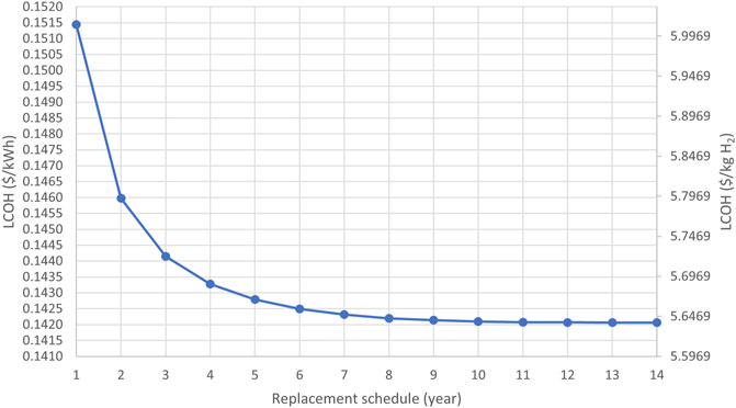
FIGURE 5. Minimum LCOHs for SOECs with different replacement schedules.

Figure 6 Illustrates the optimal membrane area sizes, average current densities, and average operating temperatures of SOECs. As shown in Eq. 6, SOECs that are supplied with higher current densities and operated at higher temperatures experience greater degradation over time. While operating cells at lower temperatures and current densities can enable longer lifetimes, the use of lower current densities results in diminished hydrogen production (Eq. 18). As such, when operating cells at lower current densities, it is necessary to use larger active membrane areas to meet the average hydrogen production constraint (Eq. 30). Although the required membrane area size increases alongside the replacement time, the need to replace SOECs less frequently in these cases makes the entire system more cost-effective.

FIGURE 6

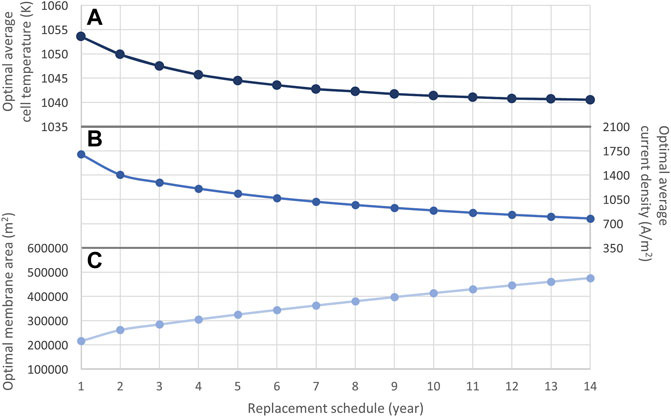
FIGURE 6. Optimal (A) average temperature, (B) average current density, and (C) average membrane area of SOECs with replacement schedules from 1 to 14 years.

Hydrogen-delivery yield increases as the fuel gas humidity is increased. As a result, the optimizer found 80% molar humidity for optimal operation of SOECs with any replacement schedule which is the maximum humidity allowed in this problem. The findings revealed that the optimal average mole recycled per mole produced is almost the same for all replacement plans (23.7%). Similarly, the optimal average voltage was also relatively the same for all cases (1.29 V). Moreover, the optimal trajectories revealed that time variations in the optimal mole recycled per mole produced and optimal voltage are insignificant. The optimal trajectories for the operating temperature and current density for the 2-, 5, and 10-years replacement plans are shown in Figure 7. For economically optimal operation, current density and temperature should reduce over the lifespan of the SOEC to lower its degradation rate. The optimal trajectories for current density in the first 2 years of operation for SOECs with 5- and 10-year replacement plans are very similar to those of an SOEC with 2-year replacement plan and they can not be discerned in this figure. Also, the optimal current density trajectories in the first 5 years of operation for an SOEC with 10-year replacement plan are very similar to those of an SOEC with 5-year replacement plan and they can not be distinguished in Figure 7. Even though the upper bound of current density was defined as 18,000 A/m², the optimal value barely reaches 1780 A/m² in the beginning of the cell’s operation and is reduced over time due to its significant influence on degradation.

FIGURE 7

FIGURE 7. Trajectories of (A) optimal current density and (B) optimal temperature of SOECs with 2-, 5-, and 10-year replacement schedules over a 20-year project lifespan.

4.2 Sensitivity analysis

As discussed in Section 4, the capital cost of SOECs varies with production volume and the cells’ commercialization status. Specifically, the capital costs of SOECs are high for non-commercial, custom-made, small-scale systems, and much lower for large-scale commercial systems. To quantify the sensitivity of the LCOH to the capital cost of SOECs, we repeated the optimization problem for capital costs of 0.12, 0.48, and 0.72 $/cm², while keeping the remaining conditions, including the other cost parameters, used in the base-case problem described in the previous section. The following trends emerged from this analysis. First, reducing the capital cost from 0.72 to 0.12 $/cm² resulted in a 21.4% decrease in the LCOH of 1-year SOECs (Figure 8A). Second, the findings showed that the impact of capital cost on the economics of the system decreases as replacement time increases. For instance, reducing the capital cost from 0.72 to 0.12 $/cm² resulted in a 6.4% and 3.5% decline in the LCOH of 5- and 14-year SOECs, respectively. Finally, the analysis showed that the tendency for LCOH to decrease as SOEC lifetime increases becomes more observable at higher capital costs. For example, the difference between the LCOHs of SOECs with various lifetimes was more distinct at the relatively high capital cost of 0.72 $/cm².

FIGURE 8

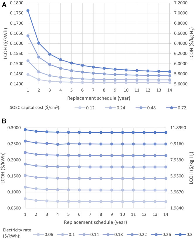
FIGURE 8. Impacts of (A) capital costs (B) electricity price on the LCOH of SOECs with various replacement schedules.

The price of electricity varies depending on a grid’s location and power generation techniques. To investigate how electricity prices influence the LCOH, we tested prices ranging from 0.06 $/kWh (the lowest rate in Canada, which is for the Quebec grid) to 0.30 $/kWh (the highest electricity rate in Canada, which is for northern grids) at 4-cent increments (Energy-Commodities, 2017; Electricity Prices in Canada, 2021). The optimization problem was solved for the different electricity prices, while all other cost values were kept the same as in the base-case problem. The results showed that the price of electricity significantly influences the LCOH, such that an 80% drop in the price of electricity results in a ∼73% decline in the LCOH (Figure 8B). As such, depending on the grid’s electricity rate, SOECs may either be an economical option for hydrogen generation or a very expensive one.

The results of the sensitivity analysis can be of great help to decision makers in selecting the proper technology for energy storage or hydrogen production in specific regions.

Figures 9A,B show the cost breakdowns of SOEC systems supplied with electricity at the lowest (0.06 $/kWh) and highest (0.30 $/kWh) prices considered in this study, respectively. The total electricity consumed at a rate of 0.30 $/kWh costs five times as much as the total electricity consumed at a rate of 0.06 $/kWh. Thus, SOECs supplied with electricity at higher price had higher capital costs than those supplied with cheaper electricity. The reason for this result is that, when electricity was expensive, the optimizer tried to lower electricity consumption by using larger SOECs and lower current densities. Since the cost of BoP also depends on the size of the cells, SOECs with more expensive electricity had higher BoP capital costs. On the other hand, the operation and maintenance costs were calculated based on the mass of hydrogen produced; thus, they were found to be almost the same for all SOECs.

FIGURE 9

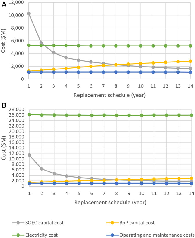
FIGURE 9. Cost breakdown of SOEC systems supplied with electricity at (A) 0.06 $/kWh and (B) 0.30 $/kWh.

5 Greenhouse gas (GHG) emissions from SOEC manufacturing and operation

Hydrogen generated through the use of electrolysers has no direct GHG emissions from the water electrolysis process. However, a more detailed environmental assessment is required to quantify the life cycle environmental impact of hydrogen production via SOECs. To this end, we calculated the life cycle GHG emissions created by the SOEC manufacturing process, as well as the life cycle GHG emissions from various electricity generation routes. A number of different grids and various primary energy sources were studied to determine how the electricity generation route impacts the environmental performance of the SOECs. The GHG emissions from the manufacturing of SOFCs was calculated in a prior work where we conducted an environmental analysis based on detailed life cycle inventory data for the manufacturing SOFCs (Naeini et al., 2021c). Since SOECs and SOFCs have the same components, the GHG emissions determined for manufacturing SOFCs in the aforementioned study (1,087 kgCO₂ eq per m² of active membrane area) were used for SOECs in the current analysis. The CO₂eq emissions from the manufacturing of BoP items are not included in this analysis due to a lack of knowledge regarding the exact size of the equipment and a lack of detailed inventory data. The power sources and power grids considered in this environmental assessment are given in Table 1. Life cycle GHG emissions of Quebec grid are almost identical to those of the hydroelectric power plant as 94% of the Quebec’s electricity is generated by hydroelectric resources (All sources of energy, 2022).

TABLE 1

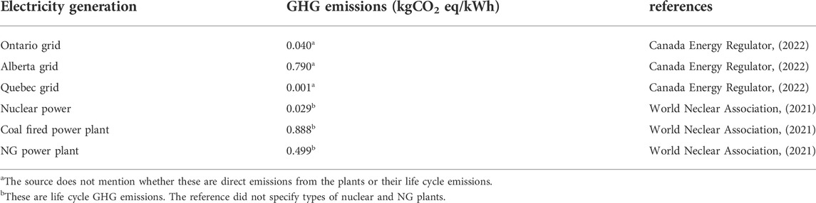
TABLE 1. Electricity generation routes studied in this work and their CO₂eq emissions.

The GHG emissions produced from the manufacturing of SOECs and the electricity supply required per kg of hydrogen generated by SOECs under optimal conditions are depicted in Figure 10. As can be seen, the electricity generation route significantly impacts the GHG emissions per mass of hydrogen produced. Moreover, SOECs with longer replacement times produce lower GHG emissions, as they require a smaller overall membrane area over the 20-year project lifespan. The life cycle GHG emissions per kg of hydrogen produced ranges from 0.34 kg CO₂eq (for 14-year SOECs connected to the Quebec grid) to 38.60 kg CO₂eq (for 1-year SOECs with coal-fired power generation). These findings demonstrate that hydrogen generated using electrolysers is not necessarily green. Even though electrolysers do not directly produce GHG emissions, they do consume a large amount of electricity; as such, the GHG emissions produced in generating this electricity should be accounted for when evaluating the electrolyser’s environmental performance. The GHG emissions of the electricity route and the price of electricity are key factors in determining whether electrolysers are the proper technology for hydrogen production in a specific region. For instance, SOECs are not an environmentally friendly option for hydrogen generation in Alberta, or in areas where electricity is generated by coal power plants. In contrast, running SOECs with electricity from the Quebec grid or nuclear power enables the production of green hydrogen, which has extremely low GHG emissions.

FIGURE 10

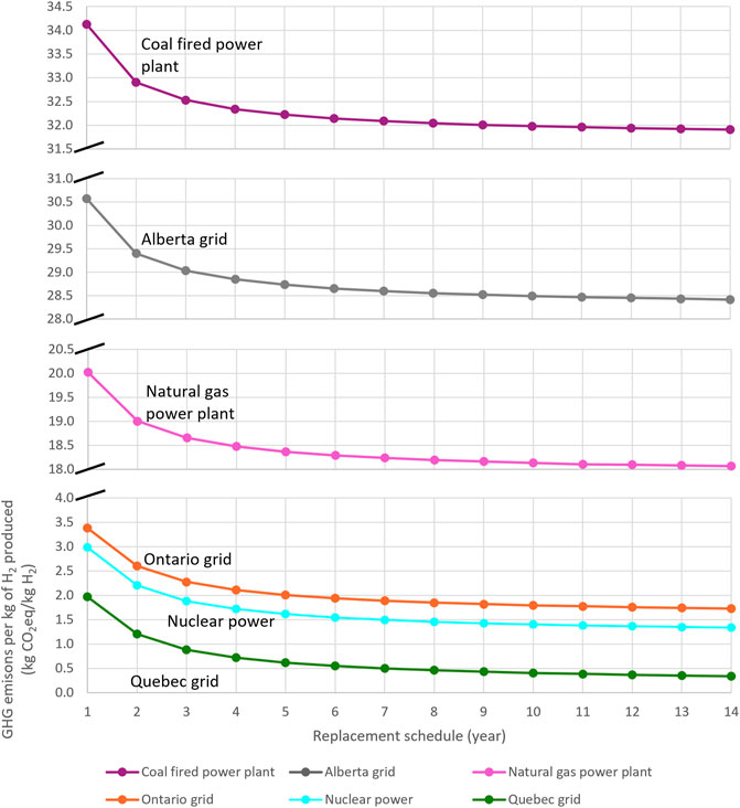
FIGURE 10. Life cycle GHG emissions per kg of hydrogen produced by SOECs with various power sources.

Figure 11 Shows a comparison of the results in the present work to other hydrogen production systems as reported in the literature. The boxes in Figure 11 show the range of as-reported life cycle CO₂eq emissions of various hydrogen-production technologies versus their LCOH. These ranges were determined by Parkinson et al. through a review of several sources (Parkinson et al., 2019). Notably, the type of electrolysers were not specified in the as-reported data. The scatter points show the results obtained for SOECs in the present study, and the impact of the replacement schedule on both the LCOH and GHG emissions is also illustrated. As can be seen, SOECs with shorter lifetimes have higher a LCOH and GHG emissions given the same power source and price of electricity. SOECs powered by low-carbon electricity have very low life cycle GHG emissions and can be competitive with existing clean technologies such as Cu-Cl cycle and S-I cycle in terms of environmental and economic metrics when the electricity is 0.06 $/kWh. Conversely, the results clearly indicate that SOECs supplied with power from the Alberta grid or coal-fired plants provide inferior environmental performance compared to other technologies. SMR, which is a mature and cost-effective hydrogen-generation route, emits between 10.72 and 15.86 kg CO₂eq per 1 kg hydrogen. SMR emissions are comparable to SOECs powered by NG, and are only exceeded by those of SOECs connected to high-carbon grids (Alberta power grid and coal-fired power plants) and coal gasification. SOECs powered by electricity from the Ontario or Quebec grids, and nuclear plant all had lower GHG emissions than SMR. The addition of carbon capture and sequestration (CCS) can reduce the life cycle GHG emissions of SMR and coal gasification by at least 45% and 64%, respectively. In addition, the highest LCOH reported for SMR and coal gasification with CCS are 1.73 and 2.75 times higher than their lowest LCOHs without CCS, respectively (Parkinson et al., 2019).

FIGURE 11

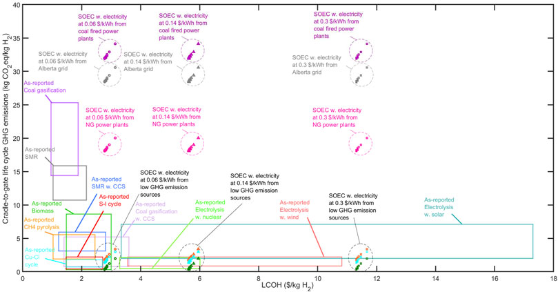
FIGURE 11. Life cycle GHG emissions of various hydrogen-production methodologies versus their LCOH. The boxes show as-reported data ranges collected by Parkinson et al. (2019) Scatter points have been calculated for SOECs in this study. Marker types indicate the electricity price. Circles, squares, and triangles indicate electricity at 0.06, 0.14, and 0.30 $/kWh, respectively. Points colors specify the supplied electricity source as follows: Coal power plant, Alberta grid, NG power plant, Ontario grid, Nuclear power, Quebec grid.

As shown in Figure 11, some technologies have large ranges of LCOH or GHG emissions, which may be due to the wide ranges of system capital costs, fuel and electricity prices, and emissions in various regions, or even the use of different assumptions in different studies. As such, this plot would benefit from standardization in which all reported values across the literature were recomputed to instead consider the exact same parameters such as system scale, energy supply chain (cost, energy type, and associated life cycle impacts), same location of construction, same quality of H₂ produced, same project and currency year, etc. However, this is beyond the scope of the present study and can be pursued in future research.

6 Cost of CO₂ avoided

The cost of CO₂ avoided (CCA) is a metric that is used to quantify the excess costs accrued from reducing CO₂eq emissions by 1 tonne compared to the base-case technology. Even though assumptions are always made in the definition of the CCAs, this metric enables comparisons of various technologies to determine the most economical and environmentally friendly option. In this study, SMR was used as the status quo system. The CCA was defined as the additional costs a technology must incur to avoid the CO₂ emissions of SMR (grey hydrogen, without CCS) over the amount of avoided CO₂ emissions (Eq. 44).

$CCA=\frac{{LCOH}_{technology}-{LCOH}_{SMR}}{{GHG}_{SMR}-{GHG}_{technology}}(44)$

where ${LCOH}_{technology}$ and ${GHG}_{technology}$ are the LCOH and GHG emissions of the investigated technology in $/tonne H₂ and tonne CO₂/tonne H₂, respectively, and ${LCOH}_{\mathrm{S}\mathrm{M}\mathrm{R}}$ and ${GHG}_{\mathrm{S}\mathrm{M}\mathrm{R}}$ are the average of the LCOHs and the GHG emissions reported by Parkinson et al. for SMR (i.e., 1,280 $/tonne H₂ and 12.4 tonne CO₂/tonne H₂). This metric is beneficial for selecting the technology that will incur the lowest costs to reduce GHG emissions. Operating costs such as fuel and electricity prices generally change based on location, as do the life cycle GHG emissions of the fuel and electricity used in these technologies. As such, the same technology can have a range of CCAs depending on where it is implemented. Table 2 presents the CCA values for SOECs on a 5-year replacement schedule operated using electricity from low-GHG-emission power sources obtained at three different prices. The CCAs of SOECs operated with electricity from the Alberta grid, coal-fired, and NG-based power plants are undefined (negative values), as they are more expensive and emit more GHGs compared to SMR.

TABLE 2

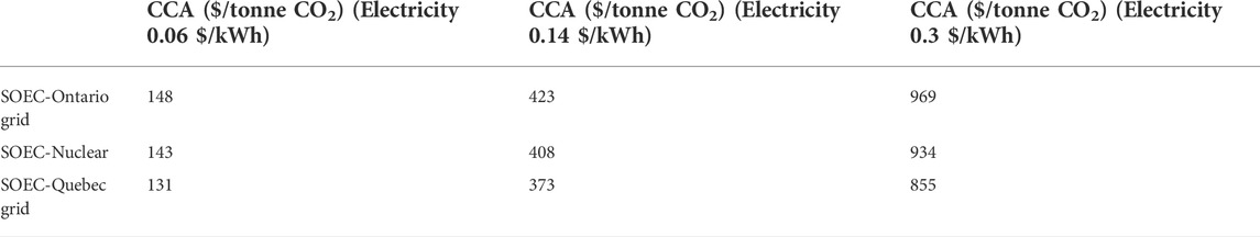
TABLE 2. CCA values for 5-year SOECs supplied with electricity from various power sources at 0.06, 0.14, and 0.3 $/kWh.

Parkinson et al. reported CCAs ranging between 97 and 110 $/tonne CO₂ for SMR systems equipped with CCS (so called “blue hydrogen”). These were calculated for supply chain emissions of 2.97–9.16 kg CO₂/kg H₂. A comparison of the CCAs listed for CCS-equipped SMR and SOECs in Table 2 indicates that, in the current market, SMR with CCS is more efficient at reducing CO₂ emissions. Although the use of SOECs to produce hydrogen results in lower GHG emissions (Figure 11), SMR with CCS remains the preferable option based on the CCA. However, this could change if the capital costs of SOEC can be reduced or if the SOEC can be supplied with less expensive electricity. It is worth noting that the SMR with CCS option requires the existence of CCS infrastructure, such as pipelines and geological sequestration, which may be difficult to achieve, especially in the short term, and so SOECs may still be the practical alternative. It is also worth noting that if the SOEC is operated only during overnight hours when the electricity demand is lower and the electricity is cheaper, the LCOH—and hence, the CCA values—of the SOEC will be significantly lower. Unfortunately, there is a paucity of long-term experiments and adequate data on how cyclic operation affects long-term SOEC degradation. The experimental data used to generate the data-driven degradation-based model in this work were collected from the continuous operation of SOECs. Therefore, the model does not predict performance degradation under cyclic operation. For these reasons, the cyclic operation of SOECs was not studied in this work.

7 Conclusion

The findings of this study revealed that it is possible to decelerate the degradation of SOECs, increase their operating lifetime, and lower their LCOH by adjusting the operating conditions. Furthermore, this study identified the optimal operating trajectories under which SOECs can be used for economical hydrogen generation over a particular length of time. This study revealed that the key to expanding the lifetime of SOECs is to gradually decrease the supplied current density and operating temperature.

A sensitivity analysis was conducted to quantify how capital costs and electricity price impact the LCOH of SOECs. The results of this sensitivity analysis can be used to determine whether SOECs are an economical option for hydrogen production in a particular region, depending on their commercial status and the price of electricity.

Lastly, this study evaluated the environmental performance of SOECs by calculating their life cycle GHG emissions per kg of hydrogen delivered. Even though electrolysers do not have direct GHG emissions, this study revealed that their life cycle GHG emissions can vary from very low levels (comparable to those of the cleanest hydrogen-production processes, such as Cu-Cl cycle) to very high amounts (more than those of the SMR process). The findings also revealed that the source of electricity has a significant impact on the environmental performance of SOECs; specifically, it was observed that SOECs may or may not be an environmentally friendly option for hydrogen production depending on how the electricity they use is generated. Finally, the CCA was calculated to help decision makers assess SOECs based on their environmental and economical performance and compare it with other technologies.

8 Future work

As mentioned previously, the widespread use of low-carbon power generators such as nuclear, solar, and wind plants is a key step toward a low-carbon future. However, the intermittency of solar and wind power limits their application compared to more consistent power sources. The scope of this study is limited to SOECs that use always-available power sources. Future work will consider wind and solar generators in combination with a variety of energy storage technologies (such as batteries, pumped hydro, or compressed air energy storage) or secondary generators such as natural gas peaking power plants to provide a consistent source of electricity. It would be interesting to determine how this impacts the economics and life cycle greenhouse gas emissions, and whether they might be suitable alternatively to those presented in the present work.

Data availability statement

The raw data supporting the conclusion of this article will be made available by the authors, without undue reservation.

Author contributions

MN: Conceptualization, methodology, data curation, formal analysis, investigation, visualization, writing—original draft. JC: Funding acquisition, project administration, supervision, writing—review and editing. TA: Conceptualization, methodology, project administration, resources, software, supervision, writing—review and editing.

Acknowledgments

We gratefully acknowledge Natural Sciences and Engineering Research Council of Canada (NSERC CRDPJ 509219-2017) and the Ontario Centre of Excellence (OCE 27851-2018) for financially supporting this research.

Conflict of interest

The authors declare that the research was conducted in the absence of any commercial or financial relationships that could be construed as a potential conflict of interest.

Publisher’s note

All claims expressed in this article are solely those of the authors and do not necessarily represent those of their affiliated organizations, or those of the publisher, the editors and the reviewers. Any product that may be evaluated in this article, or claim that may be made by its manufacturer, is not guaranteed or endorsed by the publisher.

References

All sources of energy (2022). agriculture-environment-and-natural-resources. AvaliableAt: https://www.quebec.ca/en/agriculture-environment-and-natural-resources/energy/energy-production-supply-distribution/sources-energy.

Google Scholar

Bhandari, R., and Shah, R. R. (2021). Hydrogen as energy carrier: Techno-economic assessment of decentralized hydrogen production in Germany. Renew. Energy 177, 915–931. doi:10.1016/J.RENENE.2021.05.149

CrossRef Full Text | Google Scholar

Canada Energy Regulator (2022). Régie de l’énergie du Canada. AvaliableAt: https://www.cer-rec.gc.ca/.

Google Scholar

Electricity Prices in Canada (2021). Electricity prices in Canada. AvaliableAt: https://www.energyhub.org/electricity-prices/.

Google Scholar

Energy-Commodities (2017). canadas-renewable-power-landscape. AvaliableAt: https://www.cer-rec.gc.ca/en/data-analysis/energy-commodities/electricity/report/2017-canadian-renewable-power/canadas-renewable-power-landscape-2017-energy-market-analysis-ghg-emission.html.

Google Scholar

Gallardo, F. I., Monforti Ferrario, A., Lamagna, M., Bocci, E., Astiaso Garcia, D., and Baeza-Jeria, T. E. (2021). A techno-economic analysis of solar hydrogen production by electrolysis in the north of Chile and the case of exportation from atacama desert to Japan. Int. J. Hydrogen Energy 46 (26), 13709–13728. doi:10.1016/J.IJHYDENE.2020.07.050

CrossRef Full Text | Google Scholar

Garraín, D., Banacloche, S., Ferreira-Aparicio, P., Martínez-Chaparro, A., and Lechón, Y. (2021). Sustainability indicators for the manufacturing and use of a fuel cell prototype and hydrogen storage for portable uses. Energies 202114 (20), 6558. doi:10.3390/en14206558

CrossRef Full Text | Google Scholar

Guan, X., Pal, U. B., and Powell, A. C. (2014). Energy-efficient and environmentally friendly solid oxide membrane electrolysis process for magnesium oxide reduction: Experiment and modeling. Metallurgical Mater. Trans. E 1 (2), 132–144. doi:10.1007/s40553-014-0013-x

CrossRef Full Text | Google Scholar

Habibollahzade, A., Gholamian, E., and Behzadi, A. (2019). Multi-objective optimization and comparative performance analysis of hybrid biomass-based solid oxide fuel cell/solid oxide electrolyzer cell/gas turbine using different gasification agents. Appl. Energy 233-234 (2018), 985–1002. doi:10.1016/j.apenergy.2018.10.075

CrossRef Full Text | Google Scholar

Hartvigsen, J., Petri, R., and Tao, G. (2015). DOE hydrogen and fuel cells program record. DOE Hydrog. Fuel Cells Progr. Rec. Rec. 15, 15.

Google Scholar

Hauch, A., Jensen, S., Mogensen, M., and Ramousse, S. (2006). Performance and durability of solid oxide electrolysis cells. Meet. Abstr. MA2006-01, 842. doi:10.1149/ma2006-01/24/842

CrossRef Full Text | Google Scholar

Hauch, A., Küngas, R., Blennow, P., Hansen, A. B., Hansen, J. B., Mathiesen, B. V., et al. (2020). Recent advances in solid oxide cell technology for electrolysis. Science 3702020 (6513), 370. doi:10.1126/science.aba6118

PubMed Abstract | CrossRef Full Text | Google Scholar

Hauth, M., Becker, D., and Rechberger, J. (2021). Solid oxide fuel cell - a key technology for a highly efficient energy system. MTZ Worldw. 82 (5–6), 58–63. doi:10.1007/s38313-021-0644-0

CrossRef Full Text | Google Scholar

Hoerlein, M. P., Riegraf, M., Costa, R., Schiller, G., and Friedrich, K. A. (2018). A parameter study of solid oxide electrolysis cell degradation: Microstructural changes of the fuel electrode. Electrochimica Acta 276, 162–175. doi:10.1016/j.electacta.2018.04.170

CrossRef Full Text | Google Scholar

Hubert, M. (2018). Durability of solid oxide cells: An experimental and modelling investigation based on synchrotron X-ray nano-tomography characterization. Grenoble: Université Grenoble Alpes. Doctoral dissertation.

Google Scholar

Kim, S. J., Kim, K. J., and Choi, G. M. (2015). A novel solid oxide electrolysis cell (SOEC) to separate anodic from cathodic polarization under high electrolysis current. Int. J. Hydrogen Energy 40 (30), 9032–9038. doi:10.1016/J.IJHYDENE.2015.05.143

CrossRef Full Text | Google Scholar

Klotz, D., Leonide, A., Weber, A., and Ivers-Tiffée, E. (2014). Electrochemical model for SOFC and SOEC mode predicting performance and efficiency. Int. J. Hydrogen Energy 39 (35), 20844–20849. doi:10.1016/j.ijhydene.2014.08.139

CrossRef Full Text | Google Scholar

Mastropasqua, L., Pecenati, I., Giostri, A., and Campanari, S. (2020). Solar hydrogen production: Techno-economic analysis of a parabolic dish-supported high-temperature electrolysis system. Appl. Energy 261 (2019), 114392. doi:10.1016/j.apenergy.2019.114392

CrossRef Full Text | Google Scholar

Mendoza, R. M., Mora, J. M., Cervera, R. B., and Chuang, P. Y. A. (2020). Experimental and analytical study of an anode‐supported solid oxide electrolysis cell. Chem. Eng. Technol. 43 (12), 2350–2358. doi:10.1002/ceat.202000204

CrossRef Full Text | Google Scholar

Mogensen, M. B., Chen, M., Frandsen, H. L., Graves, C., Hansen, J. B., Hansen, K. V., et al. (2019). Reversible solid-oxide cells for clean and sustainable energy. Clean. Energy 3 (3), 175–201. doi:10.1093/ce/zkz023

CrossRef Full Text | Google Scholar

Mohammadi, A., and Mehrpooya, M. (2018). Techno-economic analysis of hydrogen production by solid oxide electrolyzer coupled with dish collector. Energy Convers. Manag. 173, 167–178. doi:10.1016/J.ENCONMAN.2018.07.073

CrossRef Full Text | Google Scholar

Muellerlanger, F., Tzimas, E., Kaltschmitt, M., and Peteves, S. (2007). Techno-economic assessment of hydrogen production processes for the hydrogen economy for the short and medium term. Int. J. Hydrogen Energy 32 (16), 3797–3810. doi:10.1016/J.IJHYDENE.2007.05.027

CrossRef Full Text | Google Scholar

Mýrdal, J. S. G., Hendriksen, P. V., Graves, C., Jensen, S. H., and Nielsen, E. R. (2016). Predicting the price of solid oxide electrolysers (SOECs). Technical University of Denmark.

Google Scholar

Naeini, M., Cotton, J. S., and Adams, T. A. (2022). Data-driven modeling of long-term performance degradation in solid oxide electrolyzer cell system. Comput. Aided Chem. Eng. 49, 847–852. doi:10.1016/B978-0-323-85159-6.50141-X

CrossRef Full Text | Google Scholar

Naeini, M., Cotton, J. S., and Adams, T. A. (2021). Dynamic lifecycle assessment of solid oxide fuel cell system considering long-term degradation effects. Energy Conversion and Management 255, 115336.

Google Scholar

Naeini, M., Cotton, J. S., and Adams, T. A. (2021). Economically optimal sizing and operation strategy for solid oxide fuel cells to effectively manage long-term degradation. Ind. Eng. Chem. Res. 60, 17128–17142. doi:10.1021/acs.iecr.1c03146

CrossRef Full Text | Google Scholar

Naeini, M., Lai, H., Cotton, J. S., and Adams, T. A. (2021). A mathematical model for prediction of long-term degradation effects in solid oxide fuel cells. Ind. Eng. Chem. Res. 60 (3), 1326–1340. doi:10.1021/acs.iecr.0c05302

CrossRef Full Text | Google Scholar

NASA (2021). Compressor thermodynamics. AvaliableAt: https://www.grc.nasa.gov/www/k-12/airplane/compth.html.

Google Scholar

Ni, M., Leung, M. K. H., and Leung, D. Y. C. (2007). Parametric study of solid oxide steam electrolyzer for hydrogen production. Int. J. Hydrogen Energy 32 (13), 2305–2313. doi:10.1016/j.ijhydene.2007.03.001

CrossRef Full Text | Google Scholar

Ni, M. (2010). Modeling of a solid oxide electrolysis cell for carbon dioxide electrolysis. Chem. Eng. J. 164 (1), 246–254. doi:10.1016/j.cej.2010.08.032

CrossRef Full Text | Google Scholar

Parkinson, B., Balcombe, P., Speirs, J. F., Hawkes, A. D., and Hellgardt, K. (2019). Levelized cost of CO2 mitigation from hydrogen production routes. Energy Environ. Sci. 12 (1), 19–40. doi:10.1039/c8ee02079e

CrossRef Full Text | Google Scholar

Parra, D., Valverde, L., Pino, F. J., and Patel, M. K. (2019). A review on the role, cost and value of hydrogen energy systems for deep decarbonisation. Renew. Sustain. Energy Rev. 101, 279–294. doi:10.1016/J.RSER.2018.11.010

CrossRef Full Text | Google Scholar

Petipas, F., Brisse, A., and Bouallou, C. (2013). Model-based behaviour of a high temperature electrolyser system operated at various loads. J. Power Sources 239, 584–595. doi:10.1016/J.JPOWSOUR.2013.03.027

CrossRef Full Text | Google Scholar

Sanz-Bermejo, J., Muñoz-Antón, J., Gonzalez-Aguilar, J., and Romero, M. (2015). Part Load operation of a solid oxide electrolysis system for integration with renewable energy sources. Int. J. Hydrogen Energy 40 (26), 8291–8303. doi:10.1016/j.ijhydene.2015.04.059

CrossRef Full Text | Google Scholar

Seitz, M., von Storch, H., Nechache, A., and Bauer, D. (2017). Techno economic design of a solid oxide electrolysis system with solar thermal steam supply and thermal energy storage for the generation of renewable hydrogen. Int. J. Hydrogen Energy 42 (42), 26192–26202. doi:10.1016/j.ijhydene.2017.08.192

CrossRef Full Text | Google Scholar

Sgobbi, A., Nijs, W., De Miglio, R., Chiodi, A., Gargiulo, M., and Thiel, C. (2016). How far away is hydrogen? Its role in the medium and long-term decarbonisation of the European energy system. Int. J. Hydrogen Energy 41 (1), 19–35. doi:10.1016/J.IJHYDENE.2015.09.004

CrossRef Full Text | Google Scholar

Sohal, M. (2009). Degradation in solid oxide cells during high temperature electrolysis (No. INL/EXT-09-15617). Idaho Falls, ID: Idaho National Lab. (INL).

Google Scholar

The CONOPT Algorithm (1999). ARKI consulting & development A/S. AvaliableAt: http://www.conopt.com/Algorithm.htm.

Google Scholar

Tietz, F., Sebold, D., Brisse, A., and Schefold, J. (2013). Degradation phenomena in a solid oxide electrolysis cell after 9000 h of operation. J. Power Sources 223, 129–135. doi:10.1016/j.jpowsour.2012.09.061

CrossRef Full Text | Google Scholar

Trofimenko, N., Kusnezoff, M., and Michaelis, A. (2017). Optimization of ESC performance for Co-electrolysis operation. ECS Trans. 78 (1), 3025–3037. doi:10.1149/07801.3025ecst

CrossRef Full Text | Google Scholar

Wang, Z., Mori, M., and Araki, T. (2010). Steam electrolysis performance of intermediate-temperature solid oxide electrolysis cell and efficiency of hydrogen production system at 300 Nm3 h−1. Int. J. Hydrogen Energy 35 (10), 4451–4458. doi:10.1016/j.ijhydene.2010.02.058

CrossRef Full Text | Google Scholar

World Neclear Association (2021). Comparison of lifecycle greenhouse gas emissions of various electricity generation sources. AvaliableAt: http://www.world-nuclear.org/uploadedFiles/org/WNA/Publications/Working_Group_Reports/comparison_of_lifecycle.pdf.

Google Scholar

Yadav, D., and Banerjee, R. (2018). Economic assessment of hydrogen production from solar driven high-temperature steam electrolysis process. J. Clean. Prod. 183, 1131–1155. doi:10.1016/J.JCLEPRO.2018.01.074

CrossRef Full Text | Google Scholar

Yates, J., Daiyan, R., Patterson, R., Egan, R., Amal, R., Ho-Baille, A., et al. (2020). Techno-economic analysis of hydrogen electrolysis from off-grid stand-alone photovoltaics incorporating uncertainty analysis. Cell Rep. Phys. Sci. 1 (10), 100209. doi:10.1016/J.XCRP.2020.100209

CrossRef Full Text | Google Scholar

Zhang, H., Wang, J., Su, S., and Chen, J. (2013). Electrochemical performance characteristics and optimum design strategies of a solid oxide electrolysis cell system for carbon dioxide reduction. Int. J. Hydrogen Energy 38 (23), 9609–9618. doi:10.1016/J.IJHYDENE.2013.05.155

CrossRef Full Text | Google Scholar

Züttel, A., Remhof, A., Borgschulte, A., and Friedrichs, O. (2010). Hydrogen: The future energy carrier. Phil. Trans. R. Soc. A 368 (1923), 3329–3342. doi:10.1098/RSTA.2010.0113

CrossRef Full Text | Google Scholar

Nomenclature

${\mathit{t}}^{\prime }$ time since 200 h (h)

$\mathit{R}$ ohmic resistance (mΩ.cm²)

$\mathit{T}$ temperature (°C or K)

$\mathit{H}$ fuel gas humidity as mole fraction of water

$\mathit{i}$ current density (A/cm² or A/m²)

$\mathit{L}\mathit{C}\mathit{O}\mathit{H}$ levelized cost of hydrogen ($/kWh or $/kg H₂)

${\mathit{A}}_{\mathit{m}}$ active membrane area (m²)

$\mathit{X}$ mole of gas recycled per mole produced

$\mathbf{C}\mathbf{R}\mathbf{F}$ capital recovery factor

$\mathbf{N}$ life of the plant (year)

$\mathit{L}$ replacement schedule (year)

$\mathbf{r}$ discount interest rate

$\mathbf{H}\mathbf{H}\mathbf{V}$ higher heating value (kJ/mol)

$\mathit{C}\mathit{C}$ capital costs ($)

$\mathit{O}\mathit{C}$ non-electricity operating and maintenance costs ($)

$\mathit{E}\mathit{C}$ electricity costs ($)

$\mathit{V}$ voltage (V)

$\dot{\mathit{n}}$ molar rate (mol/h)

$\mathit{F}$ Faraday constant (C/mol)

$\mathbf{S}\mathbf{U}$ steam utilization factor

${\mathit{P}}_{\mathit{D}\mathit{C}}$ DC power (MW)

${\mathit{P}}_{\mathit{A}\mathit{C}}$ AC power (MW)

$\mathit{E}$ heat flow (MW)

${\mathit{C}}_{\mathit{p}}$ molar heat capacity (J/mol.K or kWh/kmol.K)

${\mathit{L}}_{\mathit{v}}$ latent heat of vaporization (J/mol)

$\mathit{c}\mathit{o}\mathit{m}\mathit{p}.work$ compressor work (kWh)

$\mathit{C}\mathit{W}$ compressor work per mole of gas (kWh/kmol)

$\mathit{C}\mathit{P}\mathit{R}$ compressor pressure ratio

$\mathit{Pr}$ pressure (bar)

${\mathit{R}}_{\mathit{E}\mathit{l}}$ electricity rate ($/kWh)

${\mathit{M}}_{{\mathit{H}}_{\mathit{2}}}$ molar mass of H₂ (2 kg/kmol)

$\mathit{C}\mathit{C}\mathit{A}$ cost of CO₂ avoided ($/tonne CO₂)

Greek symbols

$\mathit{\eta }$ efficiency

$\mathit{\gamma }$ specific heat ratio

Subscripts and superscripts

$\mathit{j}$ time step

$\mathit{i}\mathit{n}$ inlet

$\mathit{o}\mathit{u}\mathit{t}$ outlet

$\mathit{d}\mathit{e}\mathit{l}$ delivered gas

$\mathit{p}$ produced gas

$\mathit{c}\mathit{o}\mathit{m}\mathit{p}$ compressor

$\mathit{c}$ consumed gas