Adaptive forecasting of diverse electrical and heating loads in community integrated energy system based on deep transfer learning

The economic operation and scheduling of community integrated energy system (CIES) depend on accurate day-ahead multi-energy load forecasting. Considering the high randomness, obvious seasonality, and strong correlations between the multiple energy demands of CIES, this paper proposes an adaptive forecasting method for diverse loads of CIES based on deep transfer learning. First, a one-dimensional convolutional neural network (1DCNN) is formulated to extract hour-level local features, and the long short-term memory network (LSTM) is constructed to extract day-level coarse-grained features. In particular, an attention mechanism module is introduced to focus on critical load features. Second, a hard-sharing mechanism is adopted to learn the mutual coupling relationship between diverse loads, where the weather information is added to the shared layer as an auxiliary. Furthermore, considering the differences in the degree of uncertainty of multiple loads, dynamic weights are assigned to different tasks to facilitate their simultaneous optimization during training. Finally, a deep transfer learning strategy is constructed in the forecasting model to guarantee its adaptivity in various scenarios, where the maximum mean discrepancy (MMD) is used to measure the gradual deviation of the load properties and the external environment. Simulation experiments on two practical CIES cases show that compared with the four benchmark models, the electrical and heating load forecasting accuracy (measured by MAPE) increased by at least 4.99 and 18.22%, respectively.

1 Introduction

Integrated energy system (IES) (Cheng et al., 2018) is recognised as a potential solution for reducing carbon emissions and improving energy utilisation efficiency (Quelhas et al., 2007). In contrast to conventional independent energy systems, IES is dedicated to the integration of various energy carriers such as electricity, gas, heat, and cooling, as well as different energy technologies such as distributed generation and energy storage (Yan et al., 2021). Community integrated energy system (CIES) involves the implementation of the IES concept near the demand side. The CIES facilitates the synergy of different energy carriers, obtains higher operational flexibility, and achieves better economic and environmental performance in the simultaneous supply of various energy forms (Gianfranco et al., 2020). Owing to these advantages, the CIES plays an important role in the development of the IES and has been put into practice in many countries.

Fluctuation of loads in a CIES is a critical factor that deteriorates operational performance and increases security risks, making load forecasting technologies indispensable in the planning and operation of modern CIES (Wang et al., 2021; Yu et al., 2022). Generally, load forecasting methods focus on different timescales. Short-term load forecasting (typically day-ahead forecasting) (Daniel et al., 2022) is most commonly used in the operation of CIES for the optimization of scheduling plans (Liu, 2020; Qin et al., 2020). It is also the basis for a CIES to determine future optimal strategies for demand response (Lyon et al., 2015; Ming et al., 2020), energy trading (Fu et al., 2021), and system maintenance (Kuster et al., 2017). As the granularity of these tasks becomes more refined, the requirement for accurate load forecasting is also promoted, motivating extensive studies on novel load forecasting theories and methods.

Load forecasting methods mainly fall into two categories: the statistical methods such as regression analysis (Bracale et al., 2020) and autoregressive integrated moving average (ARIMA) (López et al., 2019), and the machine learning methods such as artificial neural networks (Wang et al., 2018), support vector machine (SVM) (Wang et al., 2016), and extreme learning machine (ELM) (Sachin et al., 2018). Deep learning (Le et al., 2015) is a new type of machine learning method, which has gained popularity in load forecasting in recent years because of its superior learning ability, adaptability, and portability. For example, the electrical loads of 42 resident users (Yang et al., 2021) were forecasted, where it was demonstrated that deep learning has a higher accuracy than back propagation (BP) neural network and extreme gradient boosting (XGBoost) method. A novel evolutionary-based deep convolutional neural network (CNN) model (Jalali et al., 2021) was proposed for intelligent load forecasting, which mainly solved the problem of finding the optimal hyperparameters of the CNN efficiently. A novel pooling-based deep recurrent neural network (RNN) (Shi et al., 2018) was proposed, which batches a group of customer load profiles into a pool of inputs, and addresses the overfitting problem by increasing data diversity and volume. A deep belief network (DBN) was improved from three aspects (Kong et al., 2020), including input data, model, and performance, to consider demand-side management (DSM) in electrical load forecasting. Variational mode decomposition (VMD) and stacking model were employed to forecast short-term electrical loads (Zhang et al., 2022). These studies have demonstrated the applicability and effectiveness of deep learning methods in the load forecasting of energy systems.

However, load forecasting in a CIES is quite different from these existing studies, that mainly focus on aggregated load forecasting at the system level (Yu and Li, 2021). There are two new challenges need to be addressed. First, the variation and uncertainty in the diverse loads of a CIES are intensified. This is due to the smaller system scale of a CIES, as well as the coupling of different energy forms that enhance the propagation of uncertainties (Li et al., 2022). The interchangeability between different energy consumptions of users, which is enabled by flexible energy conversion equipment, would also complicate the characteristics of the load profiles.

Second, it is challenging to maintain the adaptivity of the forecasting model during long-term operation of a CIES. The load diversity in a CIES is generally reduced because of its specific functions such as commercial, residential, industrial, and educational. Under these conditions, the effects of long-term factors, such as changes in seasons, energy consumption habits, total loads, and system configurations, are magnified. For example, the characteristics of the load profile usually differ during the summer, winter, and seasonal transition periods. The gradual evolution of demand restricts the continuable applicability of a single model in the load forecasting of a practical CIES. It is also difficult to train a unified model that is suitable for all scenarios because there is no guarantee that the training data over a long period share the same distribution.

A feasible solution to deal with the uncertainty in the load forecasting of a CIES is to utilize the correlations between multiple energy demands, and perform joint forecasting. For example, a multi-energy forecasting framework based on deep belief network was designed for the short-term load forecasting of integrated energy systems, in which the correlation among electrical, gas, and heating loads were considered (Zhou et al., 2020). A hybrid network based on CNN and gated recurrent unit (GRU) was proposed for the multi-energy load forecasting of the main campus of the University of Texas at Austin (Wang et al., 2020a). A CNN-Sequence to Sequence (Seq2Seq) model was developed to consider temperature, humidity, wind speed, and the coupling relationship of multiple energy carriers in the hour-ahead load forecasting (Zhang et al., 2021). Long short-term memory (LSTM) and the coupling characteristic matrix of multiple types of loads were employed to extract the inherent features of loads and improve forecasting accuracy (Wang et al., 2020b). Multi-task learning (MTL) is also widely used as a basic framework for joint load forecasting, because it improves the cognition ability of different tasks by utilizing shared layers (Zhang and Yang, 2018). This framework was employed in similar studies for joint forecasting of electrical, heating, cooling, and gas loads (Tan et al., 2019; Zhang et al., 2020). Overall, for correlated load forecasting, MTL can learn the intrinsic relationships between different types of loads and usually achieves better performance than single-task approaches. However, differences in the degree of uncertainty of various loads may hinder the simultaneous optimization of multiple tasks, which remains a problem.

For the adaptivity of forecasting models, the transfer learning method can be considered a potential solution (Pinto et al., 2022). Existing studies on transfer learning in load forecasting primarily address the problem of insufficient training samples by learning from other similar scenarios. For example, in (Lu et al., 2022), transfer learning was utilized to solve the problem of insufficient historical load data samples when smart meters have just been deployed for a short time. The historical data of similar buildings were utilized to establish a regression model for the energy consumption forecasting of different schools (Ribeiro et al., 2018). Transfer learning was introduced into the short-term forecasting of the cooling and heating loads of buildings based on the knowledge learned from typical load models (Qian et al., 2020). Different transfer learning strategies were compared for different scenarios (building types or sample sizes) in short-term forecasting of building power consumption (Fan et al., 2020). In summary, transfer learning facilitates the sharing of common features in similar learning tasks, and can be expected to solve the problem of load data expiration in a CIES caused by gradual changes over time, such as seasonal transitions.

In this study, a multi-task deep transfer learning method with an online rolling mechanism is employed to address the challenges in the load forecasting of CIES, which enables the joint day-ahead forecasting of electrical and heating loads while dynamically adapting to the varying load properties. The main contributions of this study are summarised as follows:

1) A novel framework is established for day-ahead forecasting of electrical and heating loads in a CIES. CNN and LSTM are employed to extract the features of the loads at different time scales separately. Subsequently, an attention mechanism is designed to determine the key features and track them in the forecasting results. Day-ahead weather forecasting information is considered through a shared layer to further improve accuracy.

2) A novel loss function is applied to improve the training performance of the forecasting model. In this loss function, different weights are assigned to the learning tasks of the electrical and heating loads. These weights are dynamically adjusted in the training process based on the difference in the degree of uncertainty of different types of loads, which balances the convergence speed of multiple learning tasks and facilitates their simultaneous optimization in training.

3) A deep transfer learning strategy is constructed in the forecasting model to guarantee its adaptivity in various scenarios. The maximum mean discrepancy (MMD) is used to measure the gradual deviation of the load properties and the external environment. Then, different transfer learning strategies are adopted according to the range of the MMD, which enables the forecasting model to rapidly capture the new features of the CIES.

The remainder of this paper is organized as follows. Section 2 describes the overall forecasting model, including its architecture and loss function. Section 3 details the transfer learning strategy, and summarises the entire application process. Case studies are presented in Section 4 to verify the effectiveness of the proposed method by conducting simulations using two typical cases. Finally, Section 5 concludes the paper.

2 Multi-task learning for diverse load forecasting

2.1 Architecture of the proposed multi-task learning model

As shown in Figure 1, the architecture of the proposed forecasting model can be divided into four levels. In Level-1, the multisource inputs are normalized to reduce the computational complexity and accelerate the model convergence. In Level-2, a combination of CNN, LSTM, and the attention module is employed for electrical and heating loads to extract the features at different time granularities. At this level, because weather data do not contain temporal characteristics, we directly extract weather data features through a fully connected (FC) layer. In Level-3, the features of the loads and weather data are fused together using a shared layer. Finally, in Level-4, a hard-sharing mechanism is realized using two separate FC layers with identical topologies for electrical and heating loads, through which the normalized forecasted values are simultaneously output. The forecasting results are then obtained after an inverse normalization process. Since the features have been sufficiently extracted, the output can be learned from the features of the shared layer by a simple mapping. Therefore, in this paper, the number of fully connected layers from the shared layer to the output layer is set to 1. The configurations of CNN, LSTM, and the attention mechanism are detailed in the following sections.

FIGURE 1

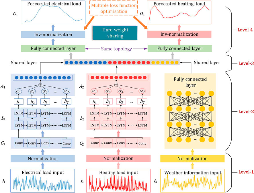
FIGURE 1. Architecture of the forecasting model.

2.1.1 One-dimensional convolutional neural network

A CNN is used to extract the fine-grained features of the loads. In this study, the input load data to the CNN is represented by time-series data. Therefore, a one-dimensional convolutional neural network (1DCNN) is adopted in the proposed model, in which the convolution operations are performed in only one dimension. The shape of a single sample input to the convolutional layer is expressed as $\left[\mathrm{t}\mathrm{i}\mathrm{m}\mathrm{e}\_\mathrm{s}\mathrm{t}\mathrm{e}\mathrm{p}\mathrm{s},\mathrm{d}\mathrm{i}\mathrm{m}\mathrm{e}\mathrm{n}\mathrm{s}\mathrm{i}\mathrm{o}\mathrm{n}\mathrm{s}\right]$, where $\mathrm{t}\mathrm{i}\mathrm{m}\mathrm{e}\_\mathrm{s}\mathrm{t}\mathrm{e}\mathrm{p}\mathrm{s}$represents a given number of days before the forecasting day, and $\mathrm{d}\mathrm{i}\mathrm{m}\mathrm{e}\mathrm{n}\mathrm{s}\mathrm{i}\mathrm{o}\mathrm{n}\mathrm{s}$ are determined by the time granularity of forecasting. In this study, we set $\mathrm{t}\mathrm{i}\mathrm{m}\mathrm{e}\_\mathrm{s}\mathrm{t}\mathrm{e}\mathrm{p}\mathrm{s}$ as 7 considering the similarity in load patterns for each week, and $\mathrm{d}\mathrm{i}\mathrm{m}\mathrm{e}\mathrm{n}\mathrm{s}\mathrm{i}\mathrm{o}\mathrm{n}\mathrm{s}$ equals to 24 to capture the hourly variation features of loads within a day.

The structure of the 1DCNN is shown in Figure 2. The convolution kernel is convolved with the input data and then summed with the corresponding bias to obtain the result of this operation. All input data are traversed according to the given step information. This process is repeated for multiple convolution kernels to obtain the final matrix, that is, the features extracted by the convolution layer. The convolution calculation process is shown in Eq. 1:

$z_l^j={\displaystyle \sum }_{i=1,p=j}^{i=T,p=j+T-1}{\mathit{w}}_l^i\cdot {\mathit{x}}_l^p+b_l(1)$

where $T$ is the given step information; ${\mathit{x}}_l^p\in {\mathbb{R}}^{1\times d}$ is the input vector at time step $p$ for the convolution operation with the $l$th convolution kernel, $d$ is dimensions of each time step; ${\mathit{w}}_l^i\in {\mathbb{R}}^{1\times d}$ is the $i$th weight parameter vector of the $l$th convolution kernel; “$\cdot$” denotes the dot product operation; $b_l$ is the corresponding bias parameter; and $z_l^j$ is the $j$th output result of the $l$th convolution operation.

FIGURE 2

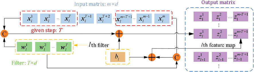
FIGURE 2. Structure of 1DCNN.

Because the 1DCNN is intended to extract hourly local features of loads within a day, we set $T$ as 1. A small number should be selected for the convolutional layers to avoid the impact of convolution operations on the original features. In addition, we choose the rectified linear unit (ReLU) as the activation function to avoid exploding gradients (Wang et al., 2020a). The numbers of network layers and convolution kernels are hyperparameters that need to be tuned in the 1DCNN.

2.1.2 Long short-term memory network

The LSTM takes the output of the CNN and is used to extract coarse-grained load features. In other words, it attempts to further learn how loads vary from day to day. The shape of a single-sample input to the LSTM is also $\left[\mathrm{t}\mathrm{i}\mathrm{m}\mathrm{e}\_\mathrm{s}\mathrm{t}\mathrm{e}\mathrm{p}\mathrm{s},\mathrm{d}\mathrm{i}\mathrm{m}\mathrm{e}\mathrm{n}\mathrm{s}\mathrm{i}\mathrm{o}\mathrm{n}\mathrm{s}\right]$, which is the same as the output of the 1DCNN.

The input of the LSTM cell at the current moment includes the input of the current moment (${\mathit{x}}_t$), hidden state of the previous moment (${\mathit{h}}_{t-1}$), and cell state (${\mathit{c}}_{t-1}$). ${\mathit{h}}_t$ and ${\mathit{c}}_t$ are reserved for the input at the next moment. These input data are processed via three types of gates, as shown in Figure 3: the forgetting gate, input gate, and output gate.

FIGURE 3

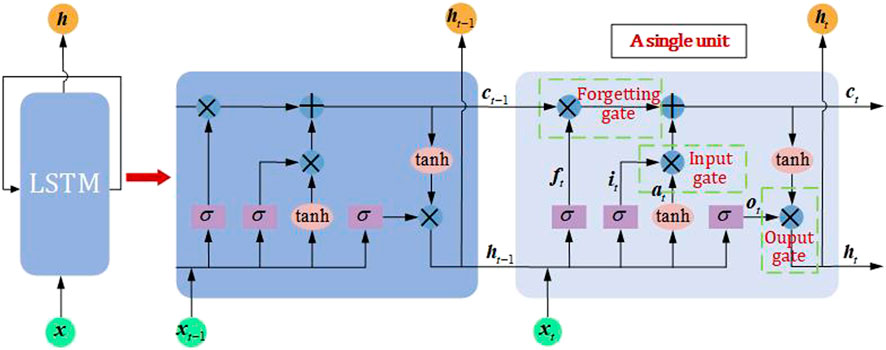
FIGURE 3. Structure of LSTM.

The equation for the forgetting gate is expressed as:

${\mathit{f}}_t=\mathbf{\sigma }\left({\mathit{W}}_f\left[{\mathit{h}}_{t-1},{\mathit{x}}_t\right]+{\mathit{b}}_f\right)(2)$

where $\mathbf{\sigma }\left(\right)$is the sigmoid function. The output range of the sigmoid function is [0,1]; therefore, ${\mathit{f}}_t$ represents the probability of forgetting the cell state at time step $t-\mathit{1}.$ ${\mathit{W}}_f$ and ${\mathit{b}}_f$ are the weights and biases of the forgetting gate, respectively.

The equation of the input gate is expressed as Eqs. 3, 4:

${\mathit{i}}_t=\mathbf{\sigma }\left({\mathit{W}}_i\left[{\mathit{h}}_{t-1},{\mathit{x}}_t\right]+{\mathit{b}}_i\right)(3)$

${\mathit{a}}_t=\mathbf{tanh}\left({\mathit{W}}_{\mathit{tan}}\left[{\mathit{h}}_{t-1},{\mathit{x}}_t\right]+{\mathit{b}}_{\mathit{tan}}\right)(4)$

where ${\mathit{W}}_i$ and ${\mathit{b}}_i$ are the weights and biases of the input gate, ${\mathit{W}}_{\mathit{tan}}$ and ${\mathit{b}}_{\mathit{tan}}$ are the weights and biases of the tanh layer. $\mathbf{tanh}\left(\right)$ denotes the activation function.

The update equation of the cell state is expressed as:

${\mathit{c}}_t={\mathit{c}}_{t-1}☉{\mathit{f}}_t+{\mathit{i}}_t☉{\mathit{a}}_t(5)$

where $☉$ denotes the Hadamard product. ${\mathit{c}}_{t-1}☉{\mathit{f}}_t$ determines whether to retain the original cell state at time step $t-\mathit{1}$, which represents the effect of the cell state at time step $t-\mathit{1}$ on the cell state at time step $t$. ${\mathit{i}}_t☉{\mathit{a}}_t$ determines whether to update the cell state at time step $t$, which represents the effect of the load at time step $t$ on the cell state at time step $t$.

The equation of the output gate is expressed as Eqs. 6, 7:

${\mathit{o}}_t=\mathbf{\sigma }\left({\mathit{W}}_o\left[{\mathit{h}}_{t-1},{\mathit{x}}_t\right]+{\mathit{b}}_o\right)(6)$

${\mathit{h}}_t={\mathit{o}}_t☉\mathbf{tanh}\left({\mathit{c}}_t\right)(7)$

where ${\mathit{W}}_o$ and ${\mathit{b}}_o$ are the weights and biases of the output gate, respectively.

The hyperparameters of LSTM include the number of network layers and the number of neurons in the hidden layer. The activation function also uses ReLU.

2.1.3 Attention mechanism module

The attention mechanism module is used to capture the temporal long-term dependencies in the load sequence (Zang et al., 2021). The core idea of the attention mechanism is to allocate more attention to important information and less attention to other information, thereby achieving the purpose of focusing on a specific region. In this study, the attention mechanism module is used to focus on historical key load features. The input of the attention mechanism module is the output vector $\mathit{h}$ processed by the LSTM activation layer. The structure of the attention mechanism module is shown in Figure 4.

FIGURE 4

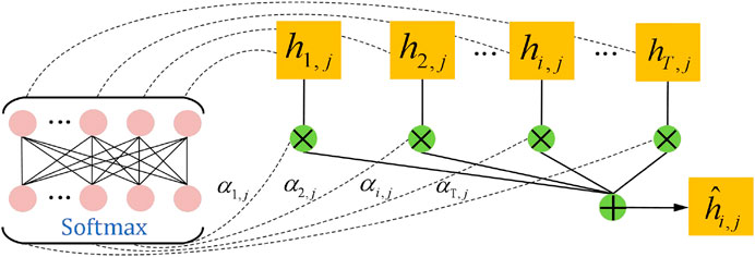
FIGURE 4. Structure of the attention mechanism.

The specific implementation of the attention mechanism can be expressed as follows:

$e_{i,j}={\tanh (\mathit{W}}_a\cdot {\mathit{h}}_j+b_a)(8)$

${\alpha }_{i,j}=\frac{\exp \left(e_{i,j}\right)}{{\sum }_{i=1}^{i=T}\exp \left(e_{i,j}\right)}(9)$

${\widehat{h}}_{i,j}={\sum }_{i=1}^{i=T}{\alpha }_{i,j}{h}_{i,j}(10)$

where $h_{i,j}$ is the $j$th output feature vector at time step $i$, ${\mathit{h}}_j=\left[h_{i,j},i=\mathit{1,2},\dots ,T\right]$, $T$ is the total time step, ${\mathit{W}}_a$ and $b_a$ are trainable weights and biases, $e_{i,j}$ is the attention score of $h_{i,j}$, ${\alpha }_{i,j}$ is the corresponding weight of $h_{i,j}$, and ${\widehat{h}}_{i,j}$ is the final output feature of attention mechanism layer.

By introducing the attention mechanism, more prominent features can achieve higher scores and thus occupy more weight in the output features. Thus, long-distance interdependent features of loads can be captured more easily.

2.2 Loss function based on uncertainty for multi-task learning

Owing to the influence of different factors such as the external environment and temperature, the uncertainty of electrical and heating loads generally varies significantly. This brings difficulty in the multi-task learning model to define a unified loss function for the training of multiple tasks.

The simplest approach is to integrate the loss functions of the different tasks and then sum them up. This approach has some shortcomings, particularly when there are significant differences in the degree of uncertainty for different tasks. For example, when the model converges, the electrical load may be more regular and performs better in forecasting, whereas the heating load is much more uncertain and exhibits poor forecasting. The reason behind this is that certain loss functions with larger magnitude dominates the entire loss function and hides the effects of loss functions with smaller magnitude. The solution to this problem is to replace the “average summation” of multiple loss functions with a “weighted summation.” Weighting can make the scale of each loss function consistent; however, it also introduces a new problem: the hyperparameter of the weight coefficient is difficult to determine.

A weight optimisation approach for MTL using uncertainty was proposed in 2018 by Kendall et al. (2018). In this study, we apply the loss function to dynamically adjust the weight coefficient during the training process, which is expressed as follows:

$L\left(W,{\sigma }_1,{\sigma }_2\right)=\frac{1}{2{\sigma }_1^2}{\Vert {\mathit{y}}_1-{\mathit{f}}^W\left(\mathit{x}\right)\Vert }^2+\frac{1}{2{\sigma }_2^2}{\Vert {\mathit{y}}_2-{\mathit{f}}^W\left(\mathit{x}\right)\Vert }^2+\log {\sigma }_1{\sigma }_2(11)$

where $\mathit{x}$ is the input data of the sample, ${\mathit{f}}^W$ denotes the MTL model (Section 2.1), ${\mathit{y}}_1$and ${\mathit{y}}_2$ are the sample labels, $W$ is the weight of the network, $\sigma$ (${\sigma \in \{\sigma }_1{,\sigma }_2\}$) is the trainable variate.

The parameters ${\sigma }_1$ and ${\sigma }_2$ are used to measure the uncertainty of different tasks, and by dividing by ${\sigma }^2$, the effect of the uncertainty of different tasks can be eliminated to some extent. It has the following advantages: 1) by dividing by ${\sigma }^2$, equivalently, different weight coefficients are assigned to different tasks, which can ensure that the individual tasks converge simultaneously; 2) $\log {\sigma }_1{\sigma }_2$ is a regular term, which prevents ${\sigma }_1$ and ${\sigma }_2$ from becoming infinitely large and ensures reliable convergence of the model; and 3) this loss function does not decrease the accuracy of the original well-performed model, but mainly optimises the parameters of the original poorly performing task.

2.3 The dropout layer and hard sharing mechanism

Owing to the small number of samples and large number of trainable parameters of LSTM, a dropout layer is added between the LSTM and attention module to prevent overfitting. During each round of training, the dropout layer discards the nodes with a certain probability. The discarded nodes are not identical each time; therefore, the structure of the model is slightly different in each training process (Srivastava et al., 2014). The dropout rate is a hyperparameter of the dropout layer.

Hard sharing is the most widely used sharing mechanism, that embeds the data representation of multiple tasks into the same space and extracts the task-specific representation for each task using a task-specific layer. Under the hard sharing mechanism, the input features are uniformly shared, and the top-level parameters of each model are independent, mainly by constructing a shared feature layer between individual tasks. Because most of the features are shared, the overfitting probability of the MTL model with the hard sharing mechanism is much smaller (Ye et al., 2022). Hard sharing is easy to implement and suitable for tasks with a strong correlation such as the coordinated load forecasting in a CIES (Wang et al., 2020a). Because features extracted from multi-source input data have been concatenated together at the shared layer, we directly use two separate fully connected layers with identical topology to quickly learn the mapping relationship between features and outputs based on the shared layer.

3 Transfer learning strategy for adaptive load forecasting

3.1 Methodology of transfer learning

For transfer learning, there are two basic concepts: the source domain $D_S$ and target domain $D_T$. The source domain is the domain with knowledge and a large number of data annotations, which represents the object to be transferred, and the target domain represents the object to which knowledge and annotations are eventually given. Tasks are also divided into source-domain tasks ${\psi }_S$ and target-domain tasks ${\psi }_T$. The transfer learning process involves transferring the knowledge of the source domain to the target domain, finding the forecasting function of the target domain, and completing the task of the target domain. Specifically, transfer learning can be divided into two categories given a labelled source domain i.e., $D_S\ne D_T$ or ${\psi }_S\ne {\psi }_T$.

A schematic of knowledge sharing for the load forecasting of a CIES is shown in Figure 5. In this paper, the centralized heating period of the CIES is considered as the source domain $D_S$ and used to initialize the forecasting model, because there is sufficient historical data, and the data distribution for each type of data (the load data and weather data) varies closely from day to day during this period. The transition season is considered as the target domain $D_T$, which has less historical data, and the distribution property for each type of data has changed from that of the centralised heating period.

FIGURE 5

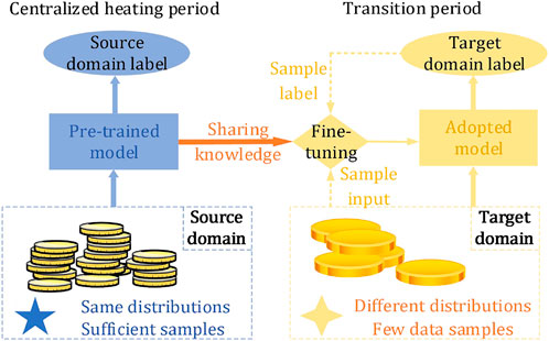
FIGURE 5. Schematic of knowledge sharing in load forecasting of CIES.

Traditional machine learning methods require sample data to be independent and identically distributed, which creates challenges for maintaining the precision of the forecasting model. At the same time, the relatively small amount of data in the transition season also limits the ability to obtain an efficient model. Fortunately, although the quantity of user demand changes gradually with the seasons, the energy usage habits of the same user are generally unchanged. Therefore, transfer learning can be introduced to reduce the difference between the source and target domains, and thus obtain an adaptive forecasting model. Here, the role of transfer learning is to extract knowledge sharing from a centralised heating period. This knowledge is then combined with the new data observed during the transition season to continuously adjust the previous model, and finally obtain the target domain model quickly and effectively.

3.2 Strategies of transfer learning based on maximum mean discrepancy

MMD is used in transfer learning mainly to measure the distribution of two different but related datasets, and is an effective method to measure the correlation of data in the source and target domains. The MMD of two datasets $\mathit{X}$ and $\mathit{Y}$ is defined as:

$\mathrm{M}\mathrm{M}\mathrm{D}\left(\mathit{X},\mathit{Y}\right)=\frac{1}{m^2}{\sum }_{i=1}^{i=m}{\sum }_{j=1}^{j=m}k\left(x_i,x_j\right)+\frac{1}{n^2}{\sum }_{i=1}^{i=n}{\sum }_{j=1}^{j=n}k\left(y_i,y_j\right)-\frac{2}{mn}{\sum }_{i=1}^{i=m}{\sum }_{j=1}^{j=n}k\left(x_i,y_j\right)(12)$

where $m$ denotes the number of $\mathit{X}$, $n$ denotes the number of $\mathit{Y}$, and $k\left(\right)$ is the kernel function.

Typically, radial basis kernel (RBF) functions are used as the kernel function:

$k\left(x_i,x_j\right)=\exp \left(-\frac{{\Vert x_i-x_j\Vert }^2}{2{\lambda }^2}\right)(13)$

where $\lambda$ denotes the width parameter of the kernel function.

It can be observed that if $\mathit{X}$ and $\mathit{Y}$ are identically distributed, $\mathrm{M}\mathrm{M}\mathrm{D}\left(\mathit{X},\mathit{Y}\right)$ is approximately zero. In other words, if $\mathrm{M}\mathrm{M}\mathrm{D}\left(\mathit{X},\mathit{Y}\right)$ is sufficiently small, the two distributions can be considered identical. Then, MMD is used as a criterion to measure the difference in the distribution of electrical and heating loads as well as weather data when seasons change.

As shown in Figure 6, the dynamic source and target domains are divided using a fixed-day sliding time window. For example, if the deviation of the model on day $t$ does not meet the pre-set forecasting accuracy, the historical data of $N$ days before day $t+1$ are considered as the target domain data, and the historical data from the previous ($M+N$) to $N$ days before day $t+1$ are considered as the source domain. $M$ and $N$ are the pre-set values of the number of days in the source and target domains, respectively. The value of M is much larger than N, so the source domain data can be used as a reference and can stably reflect the distribution of loads and weather in the previous period. The value of N is generally small; therefore, it can sensitively reflect the gradual degree of recent loads and weather. Then, the MMD values for each type of data in the source and target domains on day $t$ (${MMD}_t^{\mathrm{E}}$; ${MMD}_t^{\mathrm{H}}$; ${MMD}_t^{\mathrm{W}}$) are separately calculated using Eq. 12.

FIGURE 6

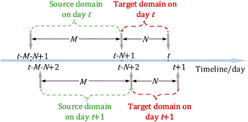
FIGURE 6. Schematic of dynamic source and target domains.

If ${MMD}_t^{\mathrm{E}}\le {\alpha }_t^{\mathrm{E}}$, ${MMD}_t^{\mathrm{H}}\le {\alpha }_t^{\mathrm{H}}$, and ${MMD}_t^{\mathrm{W}}\le {\alpha }_t^{\mathrm{W}}$, no adjustment is required to the forecasting model, where $\alpha \in \left\{{\alpha }_t^{\mathrm{E}},{\alpha }_t^{\mathrm{H}},{\alpha }_t^{\mathrm{W}}\right\}$, is the threshold value on day $t$ for different types of data. This indicates that the distributions of the source and target domains are very close. Under this condition, the forecasting model does not need to be adjusted, and forecasting deviations are mostly caused by weather anomalies on a certain day. Occasional poor performance does not indicate a substantial change in load or weather patterns in recent times.

A major advantage of using MMD is that once $M$ and $N$ are given, the thresholds for evaluating the differences in the data distribution over time can be easily obtained. For example, if the allowable average deviation of the electrical load is $R^{\mathrm{E}}$, the final $N$ days of electrical load data are multiplied by a random number uniformly distributed over $\left[1-R^{\mathrm{E}},1+R^{\mathrm{E}}\right]$ and use it as the simulation data of the target domain. The MMD of both (${\alpha }_t^{\mathrm{E}}$) is calculated as a criterion to judge whether the data distribution of electrical load in the source and target domains has changed. In this paper, the allowable average deviation of weather data $R^{\mathrm{W}}$is the same as the allowable average deviation of heating load $R^{\mathrm{H}}$.

If ${MMD}_t^{\mathrm{E}}>{\alpha }_t^{\mathrm{E}}$ or ${MMD}_t^{\mathrm{H}}>{\alpha }_t^{\mathrm{H}}$ or ${MMD}_t^{\mathrm{W}}>{\alpha }_t^{\mathrm{W}}$, it means that seasonal changes lead to variation of electrical and heating loads or user energy habits, and the transfer and fine-tuning of model parameters are performed at this time. This can be divided into two categories, as shown in Figure 7.

a) If ${MMD}_t^{\mathrm{E}/\mathrm{H}}>{\alpha }_t^{\mathrm{E}/\mathrm{H}}$ and ${MMD}_t^{\mathrm{W}}\le {\alpha }_t^{\mathrm{W}}$, using the newest data in the target domain as the new training set and fixing the other parameters of the model on day $t$, only the parameters located in the fully connected layer between the shared layer and the output layer of electrical/heating load (located in the blue/red frame of Figure 7) are fine-tuned. The fine-tuned model is used as the forecasting model on day $t+1$.

b) If ${MMD}_t^{\mathrm{W}}>{\alpha }_t^{\mathrm{W}}$, using the newest data in the target domain as the new training set and fixing the other parameters of the model on day $t$, only the parameters of all fully connected layers between the weather data and the output layer (located in the green frame of Figure 7) are fine-tuned. The fine-tuned model is used as the forecasting model on day $t+1$.

FIGURE 7

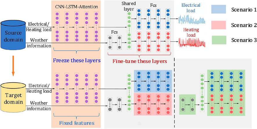
FIGURE 7. Strategies of the transfer learning.

It can be seen that the MMD helps to decide which parts of the network should be fine-tuned. For example, in Scenario a), the weather data does not change significantly, but the electrical or heating load changes significantly, which often occurs at the end of the heating period. During this period, the heating demand decreases, the central heating equipment may be turned off, and the shortfall in the heating load is replaced by other energy conversion equipment. Because the weather features are roughly unchanged, it is not necessary to adjust the parameters corresponding to the weather features. Thus, fewer parameters need to be fine-tuned, which is beneficial for the model to quickly learn dynamic changes in the target domain.

3.3 Overall framework of the proposed method

The entire online rolling forecasting process using the proposed model is shown in Figure 8. The specific steps are as follows:

FIGURE 8

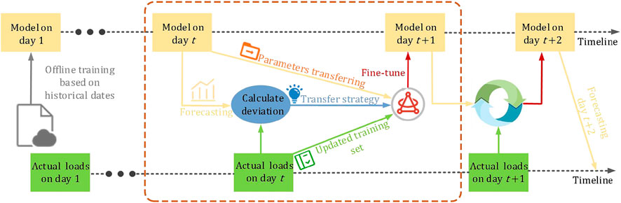
FIGURE 8. Overall framework of the proposed method.

Step 1. : Train the initial model on day 1 offline based on historical data, and use the model to forecast electrical and heating loads on day 2. Set $t=1$;

Step 2. : Forecast the load on day $t$ with the model on day $t$;

Step 3. : At the end of day $t$, electrical load deviation ${MAPE}_t^{\mathrm{E}}$ and heating load deviation ${MAPE}_t^{\mathrm{H}}$ are calculated using Eq. 14. If ${MAPE}_t^{\mathrm{E}}\le R^{\mathrm{E}}$, and ${MAPE}_t^{\mathrm{H}}\le R^{\mathrm{H}}$, the model is not adjusted and is used directly for the forecasting task on day $t+1$, where $R^{\mathrm{E}}$ and $R^{\mathrm{H}}$ are pre-set electrical and heating load accuracy thresholds;

Step 4. : If ${MAPE}_t^{\mathrm{E}}>R^{\mathrm{E}}$ or ${MAPE}_t^{\mathrm{H}}>R^{\mathrm{H}}$, the parameters are fine-tuned according to the different strategies in Section 3.2. After updating the parameters, the new model is used for the forecasting task on day $t+1$;

Step 5. : $t=t+1$, repeat Step 2 to Step 4, continuously update the model online to complete the following forecasting tasks.

4 Case studies and analysis

In this section, to demonstrate the effectiveness of the proposed method, we present simulation experiments based on real-world data of a CIES provided by the official website of the National Renewable Energy Laboratory (NREL Data Catalog, 2011) and a CIES in China. The results are compared with the following models and updating strategies:

Model-1 (no update): The model is initially trained in an offline batch manner and utilised permanently without updating.

Model-2 (daily update): The model is trained daily in a batch manner. The training set of the model keeps the number of training samples constant, continuously adding the newest observed data and eliminating the oldest data. The model adopts the structure described in Section 2.

Model-3 (single-task model, online update): This model adopts the most widely used LSTM network, and its results can be used as a reference for evaluation. The model also adopts the transfer learning strategy described in Section 3.

Model-4 (without considering the degree of uncertainty): Except for the loss function, the rest of the model is the same as in Model-5.

Model-5: The multi-tasking rolling adaptive forecasting method proposed in this study.

The determination of the hyperparameters adopts the longitudinal comparison method (Yu et al., 2021). The initial model is obtained by conducting several trials on the training set to determine optimal parameters. The longitudinal comparison method adopts the idea of the control variable method. According to the importance of each hyperparameter, the hyperparameters of different models are determined in the following priority: number of network layers–number of filters in 1DCNN—number of neurons in LSTM layer—dropout rate—number of iterations—batch size. The candidate sets for each hyperparameter are shown in Supplementary Table SA1. For example, when determining the number of layers of 1DCNN, the values of other hyperparameters are temporarily given empirically. The number of layers that minimizes the RMSE of the training set is used as the number of layers of 1DCNN and remains fixed throughout the optimization search process. Then, the next hyperparameters are determined in order of priority.

To unify the magnitudes, smooth the gradients between different batches and different layers of data, we use 0–1 normalization to normalize the data of the training set. To prevent possible changes in the maximum/minimum values when new data of the testing set are added, the maximum/minimum values for each type of data are determined based on the entire original data set, which can also prevent the effects from anomalous data. Eq. 14 is used to normalize the input data:

$x_n=\frac{x_o-x_{\mathrm{m}\mathrm{e}\mathrm{a}\mathrm{n}}}{x_{\max }-x_{\min }}(14)$

where $x_n$ is the normalized data, $x_o$ is the original data, $x_{\mathrm{m}\mathrm{e}\mathrm{a}\mathrm{n}}$, $x_{\max }$ and $x_{\min }$ are the mean, maximum, and minimum values of all data in the dataset, respectively.

The evaluation criteria used in this study are the mean absolute percentage deviation (MAPE) and root mean square error (RMSE), which are calculated as follows:

$MAPE={\sum }_{i=1}^{i=24}\frac{1}{24}\left|\frac{x_i-\widehat{x_i}}{x_i}\right|\times 100\%(15)$

$RMSE=\sqrt{{\sum }_{i=1}^{i=24}\frac{1}{24}{\left(x_i-\widehat{x_i}\right)}^2}(16)$

where $\widehat{x_i}$ is the forecasting value for the $i$th hour and $x_i$ is the actual value for the $i$th hour.

The simulation experiments for Case 1 and Case 2 are conducted under the framework of TenserFlow 2.4.1, with Intel Core i7 CPU as the hardware platform and Pycharm 2020.3 as the integrated development environment.

Case 1. : A typical park from NRELThe typical park from NREL consists of electrical, thermal, and cooling systems, with energy conversion equipment, including boilers and chillers. The dataset is composed of the hourly average electrical load, heating load, temperature, and solar radiation, collected from January 2011 to December 2011.Cosine similarity is used to measure the similarity of load patterns between weekdays and weekends, and the results are shown in Supplementary Figure SA1. The results indicate that there is a significant difference between the weekday and weekend load patterns for this park; therefore, separate forecasting models are constructed for weekdays and weekends. The data collected from 1 January 2011 to 10 February 2011 are used as the training set, and the remaining data are used as the testing set. The number of days of the source and target domains are 20 and 4, respectively. The accuracies of the electrical and heating loads are set as 8% and 12%, respectively. The optimal hyperparameters of the different models in Case 1 are presented in Supplementary Table SA2.The forecasting results of the different models during the heating period are shown in Figure 9. It is clear from Figure 9 that Model-1 has the lowest forecasting accuracy. In the first few days, its accuracy is almost identical to that of the other models, but over time, the forecasting performance of Model-1 drops dramatically. Because the training set of Model-2 is updated with time, its forecasting accuracy can be improved adaptively over a period of time; however, it also performs poorly in transition seasons and cannot fully capture the dynamic load changes over time.Figure 10 shows the forecasting results of different models in detail. It can be concluded the overall performance of Model-3 is better than Model-1 and Model-2, but there are a few time periods with large forecasting deviations that even inferior to Model-1. This is due to the fact that the single-task model does not consider the mutual coupling relationship between the electrical and heating loads and is more prone to overfitting. Figure 10 4) demonstrates that all models perform poorly when the daily fluctuation of the heating load in the transition season (from 14 February 2011 to 18 February 2011) is drastic. However, after 2 days of fine-tuning model parameters, the results of Model-5 are closest to the actual values, which indicates that Model-5 can capture the load change characteristics most quickly and stably.Figure 11 shows the distribution of RMSE of the different models. It demonstrates that that the results of Model-1 deviate significantly from the actual values and cannot be used for day-ahead forecasting throughout the year. Model-2 with the constantly updated training set has better forecasting performance in the period of smooth changes, but cannot capture load dynamics quickly when the seasonal changes are drastic. Model-3 is generally better than Model-1 and Model-2, but large deviations still occur in a few periods, which is due to the failure to consider the relationship between electrical and heating loads at the same moment. This problem makes Model-3 prone to overfitting phenomena, insufficient generalization ability and poor stability. When entering the heating period from the transition period again, Model-5 can also learn the dynamic changes of the diverse loads fastest and most stably.The specific statistics for the heating period are listed in Table 1. Combining Figure 11 with Table 1, it can be concluded that Model-5 has higher forecasting accuracy than Model-4. The performance of the two methods on the electrical load is almost the same, but the accuracy improvement of Model-5 on the heating load is more obvious. Because the Pearson correlation coefficient of the electrical and heating loads of the park is as high as 0.94, the degree of homoscedastic uncertainty between the two is comparable, so the improvement obtained by considering uncertainty is not very obvious.

FIGURE 9

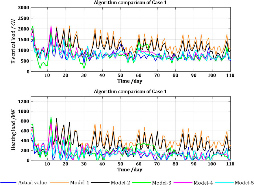
FIGURE 9. Comparison of the load forecasting results in Case 1.

FIGURE 10

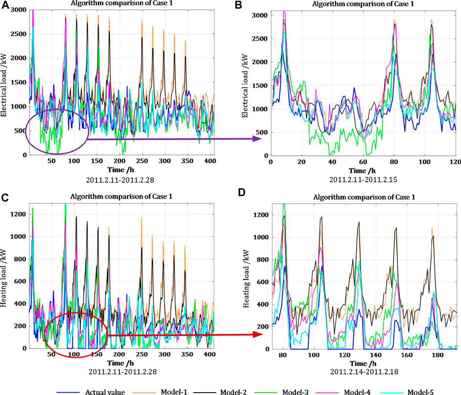
FIGURE 10. Comparison of the details in Case 1.

FIGURE 11

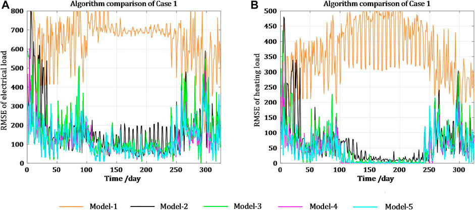
FIGURE 11. Comparison of distribution of RMSE for the different models in Case 1.

TABLE 1

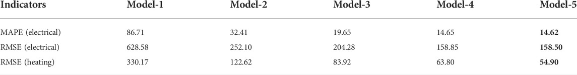
TABLE 1. Indicator results of the different models for the heating period in Case 1. The exact meaning of Model 1-5 has been given at the beginning of Section 4.

Case 2. A practical CIES in ChinaThe studied CIES in China consists of electricity, thermal and cooling systems, with energy conversion equipment including CCHP units, electrical boilers, and ground source heat pumps (Zhao et al., 2022). The dataset is composed of hourly average electrical load, heating load, temperature, photovoltaic power, solar radiation, humidity, and wind speed, collected from October 2019 to June 2020.Similarly, cosine similarity analysis shows that there is no difference between weekdays and weekends on this park; therefore, there is no need to model these cases separately. In fact, the park is operational all year round because of its business type. The Pearson correlation coefficients for diverse loads and influencing factors are shown in Supplementary Figure SA2. The influencing factors with correlation coefficients less than 0.4 (weak correlation) are not considered to avoid the influence of noise, and the final selected environment input is the temperature data.Another difference compared with Case 1 is that the correlation coefficient of the electrical and heating loads for this park is 0.63 (moderate correlation), so there is a relatively obvious difference in uncertainty between the two. The data collected from 1 October 2019 to 12 February 2020 are used as the training set, and the remaining data are used as the testing set. The optimal hyperparameters of the different models in Case 2 are listed in Supplementary Table SA3.A comparison of the electrical and heating load accuracies for each algorithm is shown in Figure 12. It is clear from Figure 12 that Model-1 and Model-2 still have the worst forecasting performance, and Model-3 still exhibits large deviations during certain periods, which is consistent with the previous conclusions of Case 1. The daily curves of the electrical load are more regular and their uncertainties are small, whereas the fluctuation of the heating load is much higher.In Figure 12 1), comparing Model-4 and Model-5, it can be concluded that the forecasting performance of the model with and without considering load uncertainty differences is comparable, which is due to the high regularity of the electrical load. The dynamic weight of the loss function corresponding to the electrical load in Model-5 is larger; therefore, the parameters corresponding to the electrical load are not easily adjusted.Figure 12 2) demonstrates that compared with Model-4, the forecasting effect of Model-5, which uses homoscedastic uncertainty to optimise the overall loss, has a significant improvement in forecasting performance, especially in the transition period. Although the RMSE of the heating load forecasted by Model-4 decreases rapidly after large deviations occur, the RMSE of the heating load forecasted by Model-5 remains at a low level. To minimise the comprehensive loss function, the weight of the heating forecasting task is smaller. This allows significant adjustment of the parameters corresponding to the heating load and effectively learns new load characteristics caused by changes in the external environment, thereby improving forecasting accuracy.The specific statistics for the heating period in Case 2 are listed in Table 2. Compared with the four models, the MAPE and RMSE of the electrical and heating loads forecasted by Model-5 decrease by at least 4.99%, 5.61%, 18.22%, and 16.72%, respectively. Figure 13 shows the number of days that meet the different forecasting precisions in Case 2. Based on a comparison of the results shown in Table 2 and Figure 13, it can be concluded that the forecasting performance of the proposed method (Model-5) is superior to that of the other methods in all aspects, both in terms of load type and different evaluation criteria. This improvement is particularly evident for the heating load forecasting task.

TABLE 2

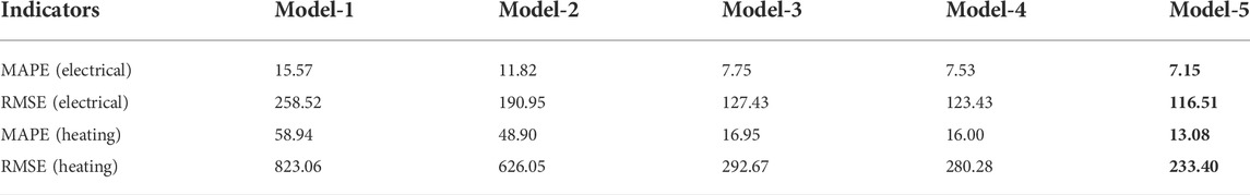
TABLE 2. Indicator results of the different models for the heating period in Case 2.

FIGURE 12

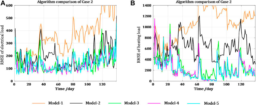
FIGURE 12. Comparison of the forecasting results in Case 2.

FIGURE 13

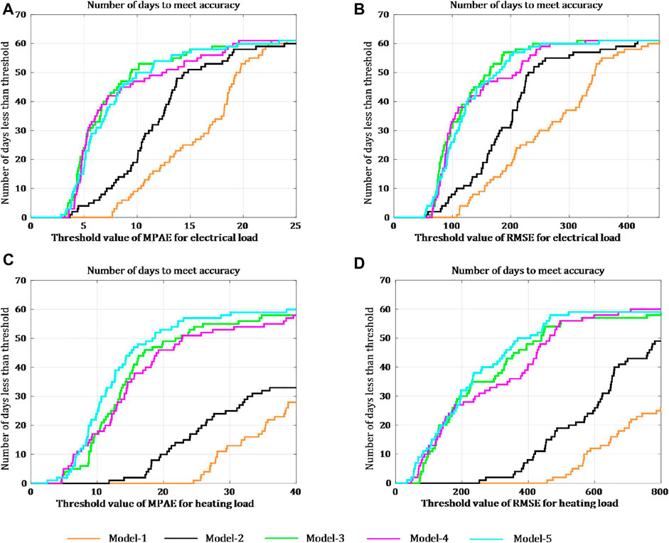
FIGURE 13. Distribution of the number of days to meet different precision.

5 Conclusion

Oriented to the adaptive multi-energy load forecasting of CIES, this paper proposes an adaptive forecasting method for diverse loads of CIES based on deep transfer learning. The proposed model uses multi-task learning to learn the interrelationships among diverse loads. CNN and LSTM are constructed to extract the features of loads at different time scales separately, and then an attention mechanism module is introduced to pay more attention to the important features. Furthermore, the dynamic weights of different tasks are assigned according to the differences in the degree of uncertainty of diverse loads to optimise the overall forecasting model. To address the adaptation of the proposed model, a deep transfer learning strategy is adopted, which enables the forecasting model to rapidly capture new CIES features. Two simulation experiments are conducted for different scenarios. The results show that the performance of the proposed method in this study is better than that of four benchmark models in forecasting diverse CIES loads. The following conclusions are drawn.

First, transfer learning is an effective method for addressing seasonal changes in CIES loads. The model without updating does not produce a consistently accurate forecast. The model whose training set is continuously updated over time can reflect the dynamic changes in load, but its performance is also poor when the load changes drastically during the seasonal transition. Second, compared to the single-task learning model, the multi-task learning model has better performance because the MTL considers the relationship between diverse loads and shares their potential information, owing to which the model has stronger generalisation ability. Finally, the MTL loss function applied in this study can improve the forecasting accuracy of the task with larger uncertainty.

Limited by the availability of data, none of the cases in this study include gas loads. In future work, CIES containing electrical, gas, and heating loads can be investigated. In addition, this study does not consider the impact of demand-side management, which can be studied further.

Data availability statement

The original contributions presented in the study are included in the article/Supplementary Material, further inquiries can be directed to the corresponding author.

Author contributions

KW: data curation, writing—original draft. HY: conceptualization and methodology. GS: formal analysis, writing—review and editing. JX: project administration. JL: investigation and software. PL: supervision and validation.

Funding

This study was supported by the National Natural Science Foundation of China (51907139, 52011530127).

Conflict of interest

The authors declare that the research was conducted in the absence of any commercial or financial relationships that could be construed as a potential conflict of interest.

The authors declare that this study received funding from Science and Technology Project of Tianjin Electric Power Company (KJ21-1-36). The funder had the following involvement in the study: JX: project administration. JL: investigation and software.

Publisher’s note

All claims expressed in this article are solely those of the authors and do not necessarily represent those of their affiliated organizations, or those of the publisher, the editors and the reviewers. Any product that may be evaluated in this article, or claim that may be made by its manufacturer, is not guaranteed or endorsed by the publisher.

Supplementary material

The Supplementary Material for this article can be found online at: https://www.frontiersin.org/articles/10.3389/fenrg.2022.1008216/full#supplementary-material

References

Bracale, A., Caramia, P., De, F., and Hong, T. (2020). Multivariate quantile regression for short-term probabil-istic load forecasting. IEEE Trans. Power Syst. 35, 628–638. doi:10.1109/TPWRS.2019.2924224

CrossRef Full Text | Google Scholar

Cheng, Y., Zhang, N., Lu, Z., and Kang, C. (2018). Planning multiple energy systems toward low-carbon society: A decentralized approach. IEEE Trans. Smart Grid 10, 4859–4869. doi:10.1109/TSG.2018.2870323

CrossRef Full Text | Google Scholar

Daniel, R., Pedro, F., Zita, V., and Regina, C. (2022). Short time electricity consumption forecast in an industry facility. IEEE Trans. Ind. Appl. 58, 123–130. doi:10.1109/TIA.2021.3123103

CrossRef Full Text | Google Scholar

Fan, C., Sun, Y., Xiao, F., Ma, J., Lee, D., Wang, J., et al. (2020). Statistical investigations of transfer learning-based methodology for short-term building energy predictions. Appl. Energy 262, 114499. doi:10.1016/j.apenergy.2020.114499

CrossRef Full Text | Google Scholar

Fu, J., Núñez, A., and Schutter, B. D. (2021). A short-term preventive maintenance scheduling method for distribution networks with distributed generators and batteries. IEEE Trans. Power Syst. 36, 2516–2531. doi:10.1109/TPWRS.2020.3037558

CrossRef Full Text | Google Scholar

Gianfranco, C., Shariq, R., Andrea, M., and Pierluigi, M. (2020). Flexibility from distributed multienergy systems. Proc. IEEE 108, 1496–1517. doi:10.1109/JPROC.2020.2986378

CrossRef Full Text | Google Scholar

Jalali, S., Ahmadian, S., Khosravi, A., Miadreza, S., Saeid, N., and João, P. (2021). A novel evolutionary-based deep convolutional neural network model for intelligent load forecasting. IEEE Trans. Ind. Inf. 17, 8243–8253. doi:10.1109/TII.2021.3065718

CrossRef Full Text | Google Scholar

Kendall, A., Gal, Y., and Cipolla, R. (2018). Multi-task learning using uncertainty to weigh losses for scene geometry and semantics. Proc. IEEE Conf. Comput. Vis. pattern Recognit. 2018, 7482–7491. doi:10.1109/CVPR.2018.00781

CrossRef Full Text | Google Scholar

Kong, X., Li, C., Zheng, F., and Wang, C. (2020). Improved deep belief network for short-term load forecasting considering demand-side management. IEEE Trans. Power Syst. 35, 1531–1538. doi:10.1109/TPWRS.2019.2943972

CrossRef Full Text | Google Scholar

Kuster, C., Rezgui, Y., and Mourshed, M. (2017). Electrical load forecasting models: A critical systematic review. Sustain. Cities Soc. 35, 257–270. doi:10.1016/j.scs.2017.08.009

CrossRef Full Text | Google Scholar

Le, C., Bengio, Y., and Hinton, G. (2015). Deep learning. Nature 521, 436–444. doi:10.1038/nature14539

PubMed Abstract | CrossRef Full Text | Google Scholar

Li, P., Li, S., Yu, H., Yan, J., Ji, H., Wu, J., et al. (2022). Quantized event-driven simulation for integrated energy systems with hybrid continuous-discrete dynamics. Appl. Energy 307, 118268. doi:10.1016/j.apenergy.2021.118268

CrossRef Full Text | Google Scholar

Liu, X. (2020). Energy stations and pipe network collaborative planning of integrated energy system based on load complementary characteristics. Sustain. Energy Grids Netw. 23, 100374. doi:10.1016/j.segan.2020.100374

CrossRef Full Text | Google Scholar

López, J., Rider, M., and Wu, Q. (2019). Parsimonious short-term load forecasting for optimal operation planning of electrical distribution systems. IEEE Trans. Power Syst. 34, 1427–1437. doi:10.1109/TPWRS.2018.2872388

CrossRef Full Text | Google Scholar

Lu, Y., Wang, G., and Huang, S. (2022). A short-term load forecasting model based on mixup and transfer learning. Electr. Power Syst. Res. 207, 107837. doi:10.1016/j.epsr.2022.107837

CrossRef Full Text | Google Scholar

Lyon, J., Wang, F., Hedman, K., and Zhang, M. (2015). Market implications and pricing of dynamic reserve policies for systems with renewables. IEEE Trans. Power Syst. 30, 1593–1602. doi:10.1109/PESGM.2015.7285837

CrossRef Full Text | Google Scholar

Ming, H., Xia, B., Lee, K., Adepoju, A., Shakkottai, S., and Xie, L. (2020). Prediction and assessment of demand response potential with coupon incentives in highly renewable power systems. Prot. Control Mod. Power Syst. 5, 12. doi:10.1186/s41601-020-00155-x

CrossRef Full Text | Google Scholar

National Renewable Energy Laboratory (NREL) Data Catalog (2011). Available at: https://data.nrel.gov/submissions/40.

Pinto, G., Wang, Z., Roy, A., Hong, T., and Capozzoli, A. (2022). Transfer learning for smart buildings: A critical review of algorithms, applications, and future perspectives. Adv. Appl. Energy 5, 100084. doi:10.1016/j.adapen.2022.100084

CrossRef Full Text | Google Scholar

Qian, F., Gao, W., Yang, Y., and Yu, D. (2020). Potential analysis of the transfer learning model in short and medium-term forecasting of building HVAC energy consumption. Energy 193, 116724. doi:10.1016/j.energy.2019.116724

CrossRef Full Text | Google Scholar

Qin, Y., Wu, L., Zheng, J., Li, M., Jing, Z., Wu, Q., et al. (2020). Optimal operation of integrated energy systems subject to coupled demand constraints of electricity and natural gas. CSEE J. Power Energy Syst. 6, 444–457. doi:10.17775/CSEEJPES.2018.00640

CrossRef Full Text | Google Scholar

Quelhas, A., Gil, E., Mccalley, J. D., and Ryan, S. M. (2007). A multiperiod generalized network flow model of the US integrated energy system: Part I-model description. IEEE Trans. Power Syst. 22, 829–836. doi:10.1109/TPWRS.2007.894844

CrossRef Full Text | Google Scholar

Ribeiro, M., Grolinger, K., Elyamany, H., Wilson, A., and Miriam, A. (2018). Transfer learning with seasonal and trend adjustment for cross-building energy forecasting. Energy Build. 165, 352–363. doi:10.1016/j.enbuild.2018.01.034

CrossRef Full Text | Google Scholar

Sachin, K., Saibal, K., and Ram, P. (2018). Intra ELM variants ensemble based model to predict energy performance in residential buildings. Sustain. Energy Grids Netw. 16, 177–187. doi:10.1016/j.segan.2018.07.001

CrossRef Full Text | Google Scholar

Shi, H., Xu, M., and Li, R. (2018). Deep learning for household load forecasting—A novel pooling deep RNN. IEEE Trans. Smart Grid 9, 5271–5280. doi:10.1109/TSG.2017.2686012

CrossRef Full Text | Google Scholar

Srivastava, N., Hinton, G., Krizhevsky, A., Sutskever, I., and Salakhutdinov, R. (2014). Dropout: A simple way to prevent neural networks from overfitting. J. Mach. Learn. Res. 15, 1929–1958.

Google Scholar

Tan, Z., De, G., Li, M., Lin, H., Yang, S., Huang, L., et al. (2019). Combined electricity-heat-cooling-gas load forecasting model for integrated energy system based on multi-task learning and least square support vector machine. J. Clean. Prod. 248, 119252. doi:10.1016/j.jclepro.2019.119252

CrossRef Full Text | Google Scholar

Wang, L., Lee, E., and Yuen, R. (2018). Novel dynamic forecasting model for building cooling loads combining an artificial neural network and an ensemble approach. Appl. Energy 228, 1740–1753. doi:10.1016/j.apenergy.2018.07.085

CrossRef Full Text | Google Scholar

Wang, S., Wang, S., Chen, H., and Gu, Q. (2020a). Multi-energy load forecasting for regional integrated energy systems considering temporal dynamic and coupling characteristics. Energy 195, 116964. doi:10.1016/j.energy.2020.116964

CrossRef Full Text | Google Scholar

Wang, X., Lee, W., Huang, H., Szabados, R., Wang, D., and Olinda, P. (2016). Factors that impact the accuracy of clustering-based load forecasting. IEEE Trans. Ind. Appl. 52, 3625–3630. doi:10.1109/TIA.2016.2558563

CrossRef Full Text | Google Scholar

Wang, X., Wang, S., Zhao, Q., Wang, S., and Fu, L. (2020b). A multi-energy load prediction model based on deep multi-task learning and ensemble approach for regional integrated energy systems. Int. J. Electr. Power & Energy Syst. 126, 106583. doi:10.1016/j.ijepes.2020.106583

CrossRef Full Text | Google Scholar

Wang, Z., Tian, Z., Li, H., and Mary, A. (2021). Predicting city-scale daily electricity consumption using data-driven models. Adv. Appl. Energy 2, 100025. doi:10.1016/j.adapen.2021.100025

CrossRef Full Text | Google Scholar

Yan, C., Bie, C., Liu, S., Urgun, D., Singh, C., and Xie, L. (2021). A reliability model for integrated energy system considering multi-energy correlation. J. Mod. Power Syst. Clean. Energy 9, 811–825. doi:10.35833/MPCE.2020.000301

CrossRef Full Text | Google Scholar

Yang, W., Shi, J., Li, S., Song, Z., Zhang, Z., and Chen, Z. (2021). A combined deep learning load forecasting model of single household resident user considering multi-time scale electricity consumption behavior. Appl. Energy 307, 118197. doi:10.1016/j.apenergy.2021.118197

CrossRef Full Text | Google Scholar

Ye, Q., Wang, Y., Li, X., Guo, J., Huang, Y., and Yang, B. (2022). A power load prediction method of associated industry chain production resumption based on multi-task LSTM. Energy Rep. 8, 239–249. doi:10.1016/j.egyr.2022.01.110

CrossRef Full Text | Google Scholar

Yu, F., Megumi, F., and Yasuhiro, H. (2021). Deep reservoir architecture for short-term residential load forecasting: An online learning scheme for edge computing. Appl. Energy 298, 117176. doi:10.1016/j.apenergy.2021.117176

CrossRef Full Text | Google Scholar

Yu, H., Tian, W., Yan, J., Li, P., Zhao, K., Wallin, F., et al. (2022). Improved triangle splitting based bi-objective optimization for community integrated energy systems with correlated uncertainties. Sustain. Energy Technol. Assess. 49, 101682. doi:10.1016/j.seta.2021.101682

CrossRef Full Text | Google Scholar

Yu, Q., and Li, Z. (2021). Correlated load forecasting in active distribution networks using spatial-temporal synchronous graph convolutional networks. IET Energy Syst. Integr. 3, 355–366. doi:10.1049/esi2.12028

CrossRef Full Text | Google Scholar

Zang, H., Xu, R., Cheng, L., Ding, T., Liu, L., Wei, Z., et al. (2021). Residential load forecasting based on LSTM fusing self-attention mechanism with pooling. Energy 229, 120682. doi:10.1016/j.energy.2021.120682

CrossRef Full Text | Google Scholar

Zhang, G., Bai, X., and Wang, Y. (2021). Short-time multi-energy load forecasting method based on CNN-Seq2Seq model with attention mechanism. Mach. Learn. Appl. 5, 100064. doi:10.1016/j.mlwa.2021.100064

CrossRef Full Text | Google Scholar

Zhang, L., Shi, J., Wang, L., and Xu, C. (2020). Electricity, heat, and gas load forecasting based on deep multitask learning in industrial-park integrated energy system. Entropy 22, 1355. doi:10.3390/e22121355

PubMed Abstract | CrossRef Full Text | Google Scholar

Zhang, Q., Wu, J., Ma, Y., Li, G., Ma, J., and Wang, C. (2022). Short-term load forecasting method with variational mode decomposition and stacking model fusion. Sustain. Energy Grids Netw. 30, 100622. doi:10.1016/j.segan.2022.100622

CrossRef Full Text | Google Scholar

Zhang, Y., and Yang, Q. (2018). An overview of multi-task learning. Natl. Sci. Rev. 5, 30–43. doi:10.1093/nsr/nwx105

CrossRef Full Text | Google Scholar

Zhao, J., Xiong, J., Yu, H., Bu, Y., Zhao, K., Yan, J., et al. (2022). Reliability evaluation of community integrated energy systems based on fault incidence matrix. Sustain. Cities Soc. 80, 103769. doi:10.1016/j.scs.2022.103769

CrossRef Full Text | Google Scholar

Zhou, B., Meng, Y., Huang, W., Wang, H., Deng, L., Huang, S., et al. (2020). Multi-energy net load forecasting for integrated local energy systems with heterogeneous prosumers. Int. J. Electr. Power & Energy Syst. 126, 106542. doi:10.1016/j.ijepes.2020.106542

CrossRef Full Text | Google Scholar