Optimal allocation of phase shifting transformer with uncertain wind power based on dynamic programming

Phase Shifting Transformer (PST) can help improve the power flow distribution of the transmission section, which can increase the wind power consumption of the grid. In order to adapt the PST allocation to the grid evolution, this paper presents a dynamic programming method to allocate PST in each planning stage of the grid optimally. The optimal allocation model of PST under a single grid seeks to maximize the wind power consumption and the Total Transfer Capacity (TTC) between areas. A calculation method for TTC of grids containing PST and wind power is proposed. The Non-Dominated Sorting Genetic Algorithm II (NSGA2) is used to solve the Pareto sets under each planning stage of the grid. Then, the optimal planning path of PST is derived based on dynamic programming. The superiority of the proposed method is demonstrated by comparing the IEEE-118 system results of dynamic and static programming.

1 Introduction

The application of new energy sources in the grid has been rapidly developed, with the continuous process of energy transition of the grid. In 2021, over 134 GW of renewable power capacity was added in China, making up 76.1% of the newly installed power generation capacity (NEA, 2022). The annual growth rate of installed wind power generation is over 25%, and wind power has become the most rapidly developing renewable energy. However, the construction cycles of the grid and wind farms are not in sync while the amount of wind power grid-connected is increasing rapidly, resulting in the limitations on wind power delivery capacity in areas where wind power is concentrated (Zhang et al., 2020).

The traditional solutions of grid strengthening have problems such as high investment costs, low utilization, and increased environmental pressure. Installing Flexible AC Transmission System (FACTS) devices is another solution (IEA, 2017). FACTS devices can improve the wind power delivery capacity by re-dispatching the power flow distribution of the transmission section. It plays a good transition role during the planning cycle of the grid. The primary FACTS devices used currently are (Ghahremani et al., 2013): Static Var Compensator (SVC), static synchronous compensator, Thyristor Controlled Series Compensator (TCSC), PST, and Unified Power Flow Controller (UPFC). Among them, PST and UPFC have a more significant impact on wind power integration (Zhang et al., 2018). Still, the installation and operation costs of PST are much lower than those of UPFC, giving a substantial economic advantage (Brilinskii et al., 2020). Installing PST in the grid can effectively improve the power flow distribution of the transmission section, thus improving the transmission capacity and wind power consumption of the grid.

Currently, many studies have proposed optimization models for the allocation of PST. The models can be divided into two categories according to their optimization objectives. The first category mainly focuses on optimizing traditional power system indicators such as active power loss, power flow balance, grid transmission capacity, and voltage profile (Preedavichit et al., 1998). In (Verboomen et al., 2008), the phase shifter distribution factor based on the DC load flow has been derived, and a method is proposed to calculate the TTC for grids containing PST. In (Sebaa et al., 2014), a multi-objective optimization model is constructed to solve the optimal allocations of PST and SVC, considering active power loss, power flow balance, and voltage stability as optimization indicators (Gerbex et al., 2001). gives the installation numbers of TCSC, Thyristor-Controlled Phase Shifting Transformer (TCPST), Thyristor-Controlled Voltage Regulator (TCVR), and SVC. The optimization objective is to maximize the network transmission power, and the optimal allocations of each device are found by a genetic algorithm. In (Kazemi and Sharifi., 2006), the optimal location of PST is found with congestion management in normal and emergency conditions, resulting in reduced production cost and increased load capacity of the power market. In (Wu et al., 2008), a group search optimizer with multiple producers is presented to optimize the positions of TCSC, TCPST, and TCVR, and their control parameters to minimize the active power loss and improve the voltage profile. In (Lima et al., 2003), an optimal model for allocating TCPST is presented. It uses mixed integer linear programming to maximize the system load capacity. However, the results of the DC optimal power flow model are subject to errors. The second category mainly focuses on the optimization of wind power consumption. In (Miranda and Alves., 2014; Zhang et al., 2021), the optimal location of PST is found to maximize wind power consumption, but the investment cost of PST is not considered, and the number of PST is limited to one (Zhang et al., 2017). proposes a bilevel optimization model to solve the optimal locations of PST in the transmission network. The upper level problem seeks to minimize the investment costs on series FACTS, the cost of wind power curtailment, and possible load shedding. The lower level problems capture the market clearing under different operating scenarios. In (Zhang et al., 2018), a bilevel optimization model for the optimal locations of TCSC and PST in the transmission network is proposed, and the uncertainty of wind power is considered. The proposed optimal models for allocations of PST and other FACTS devices only consider the case of a single grid throughout the existing studies. These studies can only compose the planning path of PST by solving for the optimal allocation scheme of each stage, which may not be the optimal path if multi-stage grid planning is considered. This paper proposes a dynamic planning method to find the optimal allocation path of PST to solve this problem, considering the grid evolution and wind power uncertainty.

In terms of PST single-stage allocation, the existing optimization models (the second category of optimization models mentioned above) only consider wind power consumption and investment cost of PST without considering the traditional optimization indicators of the power system. This paper finds that installing PST in the grid can increase the TTC of the grid while increasing the wind power consumption. However, wind power’s uncertainty will greatly affect TTC’s calculation (Wang et al., 2021), so the traditional TTC calculation method (Verboomen et al., 2008) is no longer applicable. This paper proposes a method to calculate the TTC of grids with PST and wind power. Therefore, a multi-objective optimization model is proposed to find the Pareto sets of PST allocation schemes under a single grid, considering wind power consumption, investment and operation costs of PST, and TTC as optimization indicators.

In solving the optimal allocation model of PST, existing methods are mainly divided into two categories. The first category uses mixed integer programming to solve the DC optimal power flow model (Lima et al., 2003; Zhang et al., 2018). The time required for this solution is short, but a secondary verification is necessary because of the errors. The second category uses intelligent algorithms to solve the optimal model [GA (Gerbex et al., 2001), PSO (Zhang et al., 2021), etc.], which yields more accurate results but takes more time. Since solving the PST optimal allocation model PST does not require high computational speed, NSGA2 is applied in this paper to ensure the accuracy of the results.

To sum up, this paper proposes a dynamic programming method to find the optimal path planning of PST, considering the grid evolution. First, we build a single-stage multi-objective optimization model, with wind power consumption, investment and operation costs of PST, and TTC as optimization indicators. Second, NSGA2 is used to find the Pareto sets of each grid planning stage. Then a Technique for Order Preference by Similarity to an Ideal Solution (TOPSIS) is used to calculate the adaptation values for each allocation scheme in the Pareto sets. Finally, the optimal allocation path of PST is obtained based on the dynamic programming model. The main contributions of this paper are as follows:

1) A dynamic programming method is proposed to solve the optimal allocation path of PST in multi-stage grid planning, considering wind power uncertainty.

2) A method for calculating the TTC of grids containing PST and wind power is proposed. TTC is considered as an optimization indicator for the PST single-stage allocation model.

The rest of this paper is organized as follows. Section 2 shows the main framework of the proposed method. Section 3 introduces the basic principle and steady-state model of PST. Section 4 presents the PST single-stage allocation model. The solution based on NSGA2 is demonstrated in Section 5. Section 6 describes the dynamic programming model of PST. Section 7 verifies the effectiveness of the proposed method by comparing the IEEE 118-bus system results of dynamic and static programming. Finally, the main findings of this study are summarized with some prospects for future studies in the conclusion section.

2 Main framework of the proposed method

The proposed method is developed on the main framework of dynamic programming, and the main idea is to allocate PST dynamically in the multi-stage planning of the grid. The method has two main steps, and the framework of the proposed method is given in Figure 1.

FIGURE 1

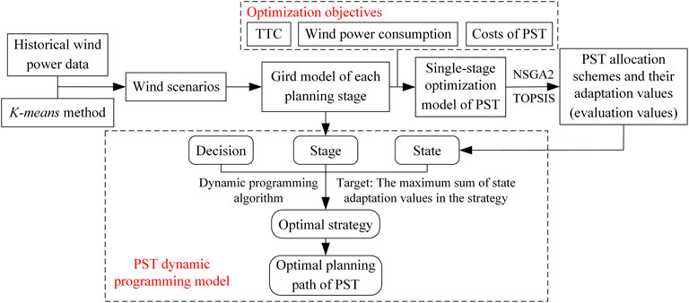
FIGURE 1. The framework of the PST allocation method.

First, the PST single-stage planning models are built for each planning stage of the grid. We consider TTC, wind power consumption, and PST costs as the optimization objectives to find the PST allocation schemes of each planning stage. TOPSIS is used to evaluate each allocation scheme by calculating its evaluation values.

Second, the dynamic programming model is constructed and solved for the optimal planning path of the PST. The dynamic planning model is built by considering each planning stage of the grid as a stage, the PST allocation scheme of each stage as a state, and the scheme’s evaluation value as the state’s adaptation value. The target is to maximize the sum of the adaptation values of the states in the strategy. Then the dynamic programming model is solved to obtain the optimal multi-stage decision, and the optimal PST planning path is obtained.

3 Basic principle and steady-state model of PST

PST changes the power flow by injecting a voltage vector into the line, resulting in the variation of the phase and voltage amplitude at both ends of the line (Ding et al., 2017). Figure 2 depicts the equivalent circuit of the branch with PST (Yeo et al., 2019), and the resistances of the line and PST are ignored here. In Figure 2, X_L represents the equivalent reactance of the line, X_eq represents the equivalent reactance of the PST, α is the phase-shift angle, and U_i, θ_i, U_j, and θ_j represent the voltage amplitude and the phase of nodes i and j, respectively. P_ij is the active power of line i-j.

${\mathit{P}}_{\mathit{i}\mathit{j}}=\frac{{\mathit{U}}_{\mathit{i}}{\mathit{U}}_{\mathit{j}}}{{\mathit{X}}_{\mathrm{L}}}\mathbf{sin}\left({\mathit{\theta }}_{\mathit{i}}-{\mathit{\theta }}_{\mathit{j}}\right),(1)$

${\mathit{P}}_{\mathit{i}\mathit{j}}=\frac{{\mathit{U}}_{\mathit{i}}{\mathit{U}}_{\mathit{j}}}{{\mathit{X}}_{\mathbf{L}}+{\mathit{X}}_{\mathbf{e}\mathbf{q}}}\mathbf{sin}\left({\mathit{\theta }}_{\mathit{i}}+\mathit{\alpha }-{\mathit{\theta }}_{\mathit{j}}\right),(2)$

FIGURE 2

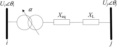
FIGURE 2. The equivalent circuit of the branch with PST.

Eqs 1, 2 represent the active power of the line before and after the installation of the PST, respectively. It can be seen that the phase angle difference has changed after the PST installation, and the active power of the line has been regulated.

4 Multi-objective optimal model of power systems with PST

4.1 Objective functions

The large-scale grid-connected wind power will increase the power flow of transmission lines, resulting in problems such as transmission line overloading and inter-regional transmission capacity limitations. The main focus of this study is to improve the wind power consumption while considering the investment cost of PST, and the TTC between grid areas is also one of the concerns.

4.1.1 Wind power consumption

The first objective function (Eq. 3) seeks to maximize the wind power consumption.

$\mathbf{max}{\mathit{f}}_{\mathbf{1}}=\frac{{\displaystyle \sum }_{\mathit{k}=\mathbf{1}}^{{\mathit{S}}_{\mathit{n}}}{\mathit{c}}_{\mathit{k}}{\mathit{W}}_{\mathit{k}}}{{\displaystyle \sum }_{\mathit{k}=\mathbf{1}}^{{\mathit{S}}_{\mathit{n}}}{\mathit{c}}_{\mathit{k}}{\mathit{W}}_{\mathit{k}\mathbf{max}}},(3)$

where c_k is the probability of scenario k. W_k and W_kmax are the wind power consumption and total wind power output under scenario k, respectively. S_n is the number of scenarios.

4.1.2 Total transfer capacity

The second objective function (Eq. 4) is to maximize the TTC between grid areas.

$\mathbf{max}{\mathit{f}}_{\mathbf{2}}=\mathit{T}\mathit{T}\mathit{C}.(4)$

We use the scenario method and linear programming to solve the TTC between the source and receiving areas. The steps are as follows:

Step 1. Use K-means clustering to reduce the number of scenarios to S_n, i = 1.

Step 2. Select a typical condition of the grid and the wind power output of scenario i is substituted into the typical condition of the grid as the base grid. The AC power flow of the base grid is calculated. Whether the wind power in the source area can be fully consumed, if so, then go to Step3; if not, then TTC is calculated as the power flow of the transmission section between the source and the receiver area.

Step 3. Calculate the sensitivity factor for line l (s_l) when the power output of all generators in the source area vary except for the balancer’s.

${\mathit{s}}_{\mathit{l}}=\frac{\mathit{d}{\mathit{P}}_{\mathit{l}}}{\mathit{d}\Delta \mathit{E}},(5)$

where $\Delta E$ denotes the variation of the power output of all generators in the source area except the balancer.

Step 4. The expression of the active power of line l is obtained based on the sensitivity factor of PST to line l.

${\mathit{P}}_{\mathit{l}}={\mathit{P}}_{\mathit{l}\mathbf{0}}+{\displaystyle \sum }_{\mathit{j}=\mathbf{1}}^{{\mathit{N}}_{\mathit{p}}}{\mathit{\alpha }}_{\mathit{j}}{\mathit{\xi }}_{\mathit{l}}^{\mathit{j}},(6)$

where ${\xi }_l^j$ denotes the sensitivity factor of the PST j to the active power of line l (Li et al., 2022a). P_l0 is the original active power of line l in the base grid. N_p is the number of PSTs installed. α_j is the phase-shift angle of PST j.

Step 5. The final active power expression for line l is obtained from Eqs 5, 6.

$\begin{array}{c}{\mathit{P}}_{\mathit{l}}={\mathit{P}}_{\mathit{l}\mathbf{0}}+{\mathit{s}}_{\mathit{l}}\cdot \Delta \mathit{E}+{\displaystyle \sum }_{\mathit{j}=\mathbf{1}}^{\mathit{N}\mathit{p}}{\mathit{\alpha }}_{\mathit{j}}{\mathit{\xi }}_{\mathit{l}}^{\mathit{j}}\end{array}.(7)$

Step 6. A linear programming model is built to maximize the TTC, with the phase shift angle and $\Delta E$ as the decision variables.

$\mathbf{max}\mathit{T}\mathit{T}{\mathit{C}}_{\mathit{i}}={\displaystyle \sum }_{\mathit{i}\in {\mathit{\Omega }}_{\mathbf{t}}}{\mathit{P}}_{\mathit{i}},(8)$

$\mathbf{s}.\mathbf{t}.\{\begin{array}{c}-{\mathit{P}}_{\mathit{l}\max }\le {\mathit{P}}_{\mathit{l}}\le {\mathit{P}}_{\mathit{l}\max },\\ {\mathit{\alpha }}_{\mathbf{min}}\le \mathit{\alpha }\le {\mathit{\alpha }}_{\mathbf{max}},\end{array}(9)$

where Ω_t denotes the regional interlink lines set, and P_lmax is the maximum permissible powers limit of line l.

Step 7. Solve the linear programming model to get the value of the phase shift angle and $\Delta E$. Then consider these values as the initial point of the Repeated Power Flow method (RPF) and obtain the value of TTC, i = i+1.

Step 8. If i = S_n, go to Step 9; If i < S_n, back to Step 2.

Step 9. Calculate the expected value with Eq. 10 considering the probability of scenarios, and the obtained expectation value is recorded as the ETTC.

$\mathbf{E}\mathbf{T}\mathbf{T}\mathbf{C}={\displaystyle \sum }_{\mathit{i}=\mathbf{1}}^{{\mathit{S}}_{\mathit{n}}}\mathit{T}\mathit{T}{\mathit{C}}_{\mathit{i}}\cdot {\mathit{c}}_{\mathit{i}}.(10)$

The RPF in Step7 is based on the conventional AC power flow, and its basic idea is as follows. From a specific base state, the output of the generation area is gradually increased while the load of the receiving area is increased correspondingly. The AC power flow in the power increasing process is repeatedly calculated. A series of power flow solution points are obtained, and various constraints are checked on these solution points until the maximum adjustment of the generator that fulfils all constraints is found. At this point, the active power of the transmission section between the transmitting and receiving areas is considered as the TTC.

4.1.3 Investment and operation costs of PST

The third objective function (Eq. 11) means to minimize the investment and operation costs of PST (Ippolito and Siano., 2004).

$\mathbf{min}{\mathit{f}}_{\mathbf{3}}={\displaystyle \sum }_{\mathit{i}=\mathbf{1}}^{{\mathit{N}}_{\mathit{p}}}{\mathit{C}}_{\mathit{P}\mathit{i}}+\mathit{\beta }\cdot {\mathit{T}}_{\mathit{i}}\cdot {\mathit{C}}_{\mathit{P}\mathit{i}},(11)$

${\mathit{C}}_{\mathit{P}\mathit{i}}=\mathit{\gamma }\cdot {\mathit{S}}_{\mathit{P}\mathit{i}},(12)$

where C_Pi is the investment cost of the PST i. β denotes the annual operating cost factor. T_i is the usage time of the PST i. γ is the cost factor of PST. S_Pi is the capacity of the PST i.

It is worth noting that the decision variables selected in the optimal model are the location of the PST, the number of PSTs, the phase shift angles, and the wind power output.

4.2 Power system constraints

4.2.1 Equation constraints

The active and reactive power constraint equations are as follows:

${\mathit{P}}_{\mathrm{G}\mathit{i}}-{\mathit{P}}_{\mathrm{L}\mathit{i}}-{\mathit{U}}_{\mathit{i}}{\displaystyle \sum }_{\mathit{j}=\mathbf{1}}^{{\mathit{n}}_{\mathit{b}}}{\mathit{U}}_{\mathit{j}}\left({\mathit{G}}_{\mathit{i}\mathit{j}}\mathbf{cos}{\mathit{\theta }}_{\mathit{i}\mathit{j}}+{\mathit{B}}_{\mathit{i}\mathit{j}}\mathbf{sin}{\mathit{\theta }}_{\mathit{i}\mathit{j}}\right)=\mathbf{0}(13)$

${\mathit{Q}}_{\mathrm{G}\mathit{i}}-{\mathit{Q}}_{\mathrm{L}\mathit{i}}-{\mathit{U}}_{\mathit{i}}{\displaystyle \sum }_{\mathit{j}=\mathbf{1}}^{{\mathit{n}}_{\mathit{b}}}{\mathit{U}}_{\mathit{j}}\left({\mathit{G}}_{\mathit{i}\mathit{j}}\mathbf{sin}{\mathit{\theta }}_{\mathit{i}\mathit{j}}-{\mathit{B}}_{\mathit{i}\mathit{j}}\mathbf{cos}{\mathit{\theta }}_{\mathit{i}\mathit{j}}\right)=\mathbf{0}(14)$

where P_Gi and Q_Gi are the active and reactive power output of the i-bus generator, respectively. P_Li and Q_Li are the load active and reactive power of the bus i. n_b is the number of lines connected to node i. G_ij and B_ij are the conductance and the susceptance of the line i-j, respectively.

4.2.2 Inequality constraints

Inequality constraints for the active and reactive power outputs of generators, voltage amplitudes of buses, and active power of branches are as follow:

$\{\begin{array}{c}\begin{array}{c}{\mathit{U}}_{\mathit{i}\mathbf{min}}\le {\mathit{U}}_{\mathit{i}}\le {\mathit{U}}_{\mathit{i}\mathbf{max}},\\ {\mathit{P}}_{\mathbf{G}\mathit{i}\mathbf{min}}\le {\mathit{P}}_{\mathbf{G}\mathit{i}}\le {\mathit{P}}_{\mathrm{G}\mathit{i}\max },\end{array}\\ \begin{array}{c}{\mathit{Q}}_{\mathbf{G}\mathit{i}\mathbf{min}}\le {\mathit{Q}}_{\mathbf{G}\mathit{i}}\le {\mathit{Q}}_{\mathrm{G}\mathit{i}\max },\\ -{\mathit{P}}_{\mathit{i}\mathit{j}\max }\le {\mathit{P}}_{\mathit{i}\mathit{j}}\le {\mathit{P}}_{\mathit{i}\mathit{j}\max },\end{array}\end{array}(15)$

where U_imax and U_imin are the maximum and minimum voltage of node i, respectively. P_Gimax and P_Gimin are the maximum and minimum active power output of generator i, respectively. Q_Gimax and Q_Gimin are the maximum and minimum reactive power output limits of generator i, respectively. P_ijmax is the maximum permissible powers limit of line i-j.

Since this paper focuses on the PST allocation in multi-stage grid planning, the time scale between the stages is in years, so the model of the generator is moderately simplified. It is assumed that the responsiveness of conventional power sources is strong enough to consume wind power. So some temporal constraints are not considered, such as ramping constraints of generators.

4.3 Constraints of decision variables

It is known that the PST is mainly used to regulate the power flow of the transmission section where PST is installed (Hadzimuratovic and Fickert., 2018). We have imposed some limits on the range of locations and the number of PSTs to avoid solving unreasonable PST allocation schemes, which are shown as follows.

1) The locations of PST are limited to the transmission sections, which contain the wind power transmission lines.

2) The maximum number of PSTs installed on a line is 1, and the maximum number of PSTs installed in a transmission section is 2.

4.3.1 Locations of PST

${\mathit{l}}_{\mathit{p}}\in \mathit{D}.(16)$

l_p is the line with PST installed. D is the set of transmission sections that deliver wind power.

4.3.2 Shift-phase angle

${\mathit{\alpha }}_{\mathbf{min}}\le \mathit{\alpha }\le {\mathit{\alpha }}_{\mathbf{max}}.(17)$

α_max and α_min are the maximum and minimum phase angles of PST, respectively.

4.3.3 Number of PSTs

Installing PST in the transmission section can improve transmission capacity by lessening the power flow of heavily loaded lines. Since the number of heavy load lines on a specific transmission section is limited, the transmission capacity enhancement will naturally decrease as more PSTs are installed (numerical simulations are performed in Section 7.5 to verify this view).

The number of lines in the transmission section is limited in the real grid. Considering the economics of PST investing, this study limits the PSTs number of the transmission section to less than 2.

${\mathit{N}}_{\mathit{i}}\le \mathbf{2}.(18)$

N_i is the PSTs number of the transmission section-i.

4.3.4 Wind power output

$\mathbf{0}\le {\mathit{P}}_{\mathit{w}\mathit{i}}\le {\mathit{P}}_{\mathit{w}\mathit{i}\mathbf{max}}.(19)$

P_wi and P_wimax are the actual and maximum output of wind power at node i, respectively.

5 Solution approach

The NSGA2 algorithm is used to solve the Pareto sets of the PST optimal allocation model. The phase shift angle and wind power output in the initial population are randomly generated, which may result in unsolvability or unreasonable power flow results [power flow reverse (Li et al., 2022)]. The following improvements are added to NSGA2 to solve this problem, and the flow chart of NSGA2 is shown in Figure 3.

1) An additional judgment is added to eliminate the unreasonable allocation schemes.

2) According to the power flow regulation characteristics of PST, the unreasonable range of phase shift angle is eliminated to accelerate the iteration speed of NSGA2

$\{\begin{array}{c}\mathbf{0}<{\mathit{\alpha }}_{\mathit{i}}\le {\mathit{\alpha }}_{\mathbf{max}}\dots \mathit{i}\in {\mathit{\Omega }}_{\mathbf{p}},\\ {\mathit{\alpha }}_{\mathbf{min}}\le {\mathit{\alpha }}_{\mathit{i}}<\mathbf{0}\dots \mathit{i}\in {\mathit{\Omega }}_{\mathbf{q}}.\end{array}(20)$

FIGURE 3

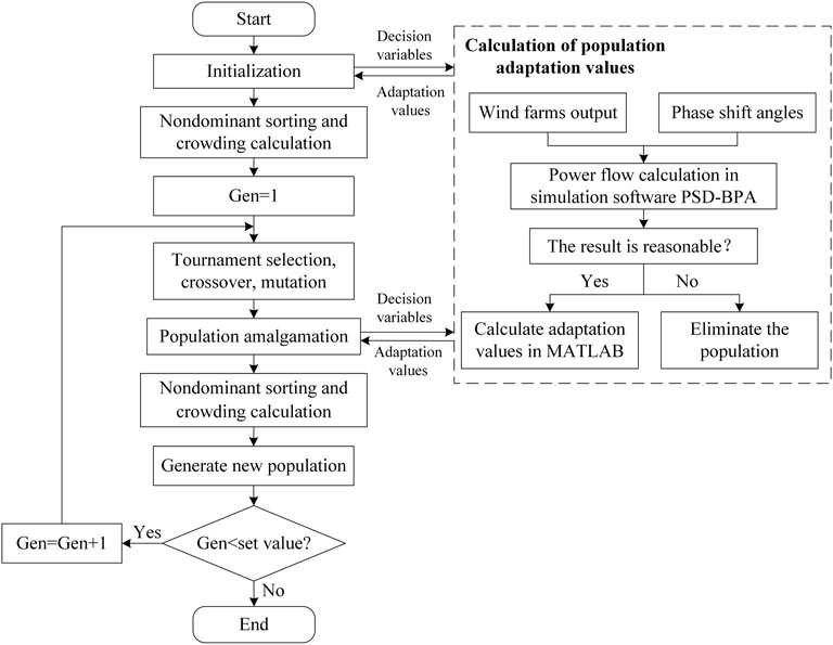
FIGURE 3. The flow chart of the multi-objective optimization model solving.

In Eq. 20, Ω_p denotes the set of lines with the lowest load factor of each wind power transmission section, so set α > 0 (Over-regulation, increasing the active power of the line). Ω_q denotes the set of lines with the highest load factor of each wind power transmission section, so set α < 0 (Hysteresis-regulation, reducing the active power of the line).

After obtaining the Pareto set by NSGA2, the scores of allocation schemes in the Pareto set are found by the TOPSIS method considering the weight coefficients.

6 PST allocation based on dynamic programming

A dynamic programming model of PST is proposed to find the optimal planning path for PST. It ensures that the allocation of PST can be better adapted to the grid evolution. Figure 4 gives the PST dynamic programming model, and the details are as follows.

Stage: Define a stage as the transformation between two adjacent planning stages of the grid, and the number of planning stages is n.

State: Define states as the PST allocation schemes of each planning stage of the grid. In Figure 4, Y_i-j indicates the jth PST allocation scheme under the ith planning stage of the grid.

Decision: The decisions represent the transition choices of PST allocation schemes between two adjacent planning stages of the grid, which are described in Figure 4 as connections between neighboring states. In addition, the set of lines with PST installed in the allocation scheme after the decision must include that of the allocation scheme before the decision (without considering the case of decommissioning or replacement of PST). In Figure 4, J_i is the number of decisions for stage i.

Strategy: Define each complete planning path through all planning stages as a strategy, represented in Figure 4 as a complete concatenation from Y₀ to Y_n.

Target: The target is to select the optimal planning path with the maximum sum of adaptation values. In Figure 4, S_i-p-q is the adaptation value of decision Y_(i-1)-p-Y_i-q at the current stage i, obtained by the TOPSIS. The specific calculation is as follows.

Step 1: Define all decisions in the current stage as evaluation objects and take the three objective functions in Section 4.1 as evaluation criteria.

$\mathbf{min}{\mathit{f}}_{\mathbf{3}}={\displaystyle \sum }_{\mathit{i}=\mathbf{1}}^{{\mathit{N}}_{\mathit{p}}}\left({\mathit{C}}_{\mathit{P}\mathbf{2}}-{\mathit{C}}_{\mathit{P}\mathbf{1}}\right)+\mathit{\beta }\cdot \mathit{m}\cdot {\mathit{C}}_{\mathit{P}\mathbf{2}}.(21)$

FIGURE 4

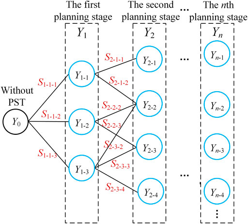
FIGURE 4. PST dynamic programming model.

Equation Eq. 21 shows the improved expression of the cost objective function, where m is the time of a stage. C_P1 and C_P2 denote the PST investment cost of the PST allocation scheme before and after the decision, respectively.

Step 2: Use the TOPSIS to obtain the unnormalized scores of all decisions in the current stage.

Step 3: Scores of all decisions at the current stage are processed as in Equation Eq. 22, ensuring that the decision scores of each stage are in the same order of magnitude.

${\mathit{S}}_{\mathit{i}-\mathit{j}}={\mathit{h}}_{\mathit{i}}\cdot {\mathit{J}}_{\mathit{i}}\cdot \frac{{\mathit{S}}_{\mathit{j}}}{{\displaystyle \sum }_{\mathit{n}=\mathbf{1}}^{{\mathit{J}}_{\mathit{i}}}{\mathit{S}}_{\mathit{n}}},(22)$

${\mathit{h}}_{\mathbf{1}}>{\mathit{h}}_{\mathbf{2}}>{\mathit{h}}_{\mathbf{3}}\cdots >{\mathit{h}}_{\mathit{n}},(23)$

where S_i is the unnormalized score of decision i. S_i-j is the normalized score of decision j in stage i. h_i is the weighting factor of stage i in all stages, reflecting the importance of each grid planning stage. Since the PST plays a transitional role in the grid planning process, the demand for PST becomes smaller as the grid evolves. So we set continuous decreasing weighting factors for successive planning stages, as shown in Equation Eq. 23. The weighting factors values of grids are derived from experience in this study.

In conclusion, the flowchart of the proposed PST dynamic programming method is shown in Figure 5. The steps are as follows.

Step 1: Build a multi-stage planning model of the grid.

Step 2: Build the optimal allocation model of PST for each planning stage (Section 4).

Step 3: Use NSGA2 to solve the optimal allocation model based on the interaction between PSD-BPA (a simulation software that is used to calculate the power flow in this paper) and a calculation procedure in MATLAB (Tao et al., 2013). The scores of the allocation schemes are obtained by the TOPSIS method considering the weight coefficients (Section 5).

Step 4: Each planning stage’s allocation schemes are considered states in the dynamic programming model. Each allocation scheme’s score is recorded as the adaptation value of each state in the PST dynamic programming model. The optimal planning path of PST is obtained by the dynamic programming algorithm (Section 6).

FIGURE 5

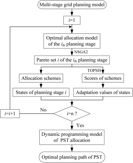
FIGURE 5. Flowchart of the PST dynamic programming method.

7 Case study

7.1 Case parameters and wind scenarios

The proposed dynamic programming model and solution approach are tested on the IEEE 118-bus system. The system data is derived from the IEEE standard system. The thermal limits for the transmission lines refer to the values in (Blumsack., 2006). Three wind farms with a maximum capacity of 1600 MW each are assumed to be located at bus 5, 26, and 91 (Ziaee and Choobineh., 2017). The phase shift angle range is set to be (−50°, 50°). The usage time of PST is set to be 15 years (the time of a complete planning path in this study). The cost factor of PST is selected to be 10$/kVA, and the annual operating cost factor is chosen to be 5%.

We built a multi-stage planning grid model in this case. Three planning stages are considered base on the IEEE 118-bus system, and the cycle between two adjacent stages is 5 years. The specific grid models of each stage are as follows.

The first planning stage: Based on the IEEE 118-bus system, the wind farm with the maximum capacity of 1600 MW is located in bus 5, and the load has increased by 20%, h₁ = 1.

The second planning stage: Based on the grid of the first planning stage, the wind farm with the maximum capacity of 1600 MW is located in bus 26, and the load has increased by 10%, h₂ = 0.9.

The third planning stage: Based on the grid of the second planning stage, the wind farm with the maximum capacity of 1600 MW is located in bus 91. The load in area C (Zhang and Grijalva., 2013) has increased by 10%, and a new transmission line has been added between bus 91 and bus 92, with line parameters consistent with the original lines of bus 91 and bus 92, h₃ = 0.8.

To obtain the wind scenarios, the wind power intensities of each 5 minutes in 7 years provided by DR POWER (National Energy Renewable Laboratory, 2019) are used to represent the wind generation profile. We then use the K-means method (Baringo and Conejo., 2013) to conduct the scenario reduction, where the optimal number of clusters is obtained by the Elbow Method (Bandara et al., 2019). The SSE distribution plots for different S_n values are shown in Figure 6.

FIGURE 6

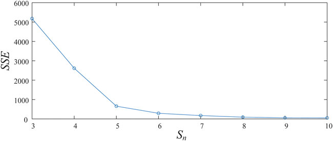
FIGURE 6. Distribution chart of SSE and S_n.

The optimal number of clusters was found to be 5, based on the results in Figure 6 and the Elbow Method. The probabilities and wind intensities for the final five scenarios are provided in Table 1.

TABLE 1

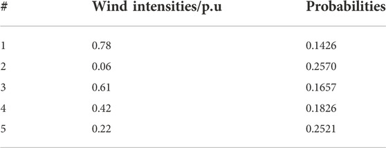
TABLE 1. Wind scenarios.

7.2 Optimal planning path of PST

In terms of NSGA2 parameters, the initial population is set to be 300, the number of iterations is set to 200, the crossover rate is set to be 0.9, and the variation rate is set to be 0.1. The normalized weight of three evaluation criteria are set to be 0.6, 0.2, and 0.2, respectively.

The Pareto sets of PST allocation for three planning stages are derived from the optimization calculation in Section 5 (the results are shown in Supplementary Tables S1–S3 in the Supplementary Material).

The proposed PST dynamic programming method is a multi-stage decision-making problem, and the connection between each stage is considered. The existing PST allocation methods are mainly used for single-stage optimization. When they are used to solve multi-stage problems, the optimal PST allocation scheme of each stage needs to be found separately and combined into a planning path by order. We define this method as static programming and the result as the static planning path.

Table 2 provides the planning results based on the static planning and the dynamic planning for Road₁ (the static planning path) and Road₂ (the dynamic planning path), respectively. Columns 2–4 indicate the wind power consumption of each wind farm. The fifth column shows the locations of the PST. The sixth column represents the investment cost of PST. The seventh column denotes the TTC between areas A and B (Zhang and Grijalva., 2013). The last column gives the wind power consumption rate of all wind farms. Doublelines 89-92 (1) and 89-92 (2) denote the lines with smaller and larger impedances between bus 89 and bus 92, respectively. Figure 7 shows the wind power curtailment rate for the three wind farms in each scenario.

TABLE 2

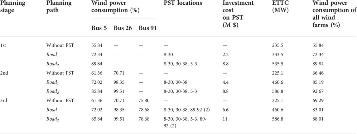
TABLE 2. IEEE 118-bus system results for different planning paths of PST.

FIGURE 7

FIGURE 7. Wind power spillage for each scenario (A) Bus 5 (B) Bus 26 (C)Bus 91.

As observed in Table 2 and Figure 7, the consumption rate of wind power under Road₁ and Road₂ has been significantly improved, and the TTC has also been improved. The wind power consumption rate and TTC of each planning stage in Road₂ are higher than those in Road₁. However, the costs of the three planning stages are higher in Road₂, resulting in a better allocation scheme in Road₁ than in Road₂ when the grid of each planning stage is considered separately.

7.3 Comparison of dynamic programming and static programming

In this section, two comparison cases are proposed to verify the effectiveness of the dynamic programming method proposed in this paper. Both cases compare the results of multi-stage allocation of PST based on static and dynamic programming.

7.3.1 Comparison case 1

The first comparison case uses the single-stage allocation model in Section 4, and the results are presented in Table 3. It compares the IEEE 118-bus system results of Road₁ and Road₂. The second column indicates the wind power consumption rate for 15 years, namely the time of a complete path in dynamic programming. The third column gives the annual average TTC value. The fourth column shows the total costs of PST in 15 years. The last column represents the sum of adaptation values.

TABLE 3

TABLE 3. IEEE 118-bus system results of Road₁ and Road₂.

As observed in Table 3, the improvement of wind power consumption under Road₂ is 11.94% higher than that under Road₁. The increase in TTC of Road₂ is 47.36% higher than that of Road₁. The sum of adaptation values under Road₂ is higher than that under Road₁, although the total costs under Road₂ are higher than that under Road₁, which means that the planning path obtained from the dynamic programming scheme is better than that of the static programming.

7.3.2 Comparison case 2

To further demonstrate the superiority of the proposed dynamic approach, the single-stage optimization model in Section 4 is replaced with the single-stage PST allocation model in (Zhang et al., 2018) while the dynamic programming framework remains unchanged in this case. Then the results of the dynamic and static programming are compared. The optimal allocation model in (Zhang et al., 2018) converts wind curtailment into the corresponding cost by using the cost coefficient of wind curtailment. The multi-objective optimization is converted to a single-objective optimization by considering the sum of the annual wind curtailment cost and the annualized investment cost in PST as the total optimization objective. Therefore, compared to the case1 in Section 7.3.1, there is no need to evaluate the allocation schemes of each stage, and the total costs of the planning path can be obtained by directly summing the costs of all stages according to their weights. Using this result to compare the effects of various planning paths is more intuitive.

The results of the second case are shown in Table 4. The objective value in Table 4 represents the annualized investment cost in PST plus the annual wind curtailment cost. In Table 4, Road₃ represents the static planning path obtained based on the static programming method, and Road₄ represents the dynamic planning path obtained based on the proposed dynamic programming method.

TABLE 4

TABLE 4. IEEE 118-bus system results of Road₃ and Road₄.

As observed in Table 4, the wind power consumption rate is higher under Road₄ than Road₃. The objective value of Road₄ is $8.141M, which is lower than the objective value of Road₃ at $9.139M, which means the planning path under the dynamic programming is better since the sum of the costs for annualized investment in PST and annual wind curtailment lower. So the proposed dynamic planning method is still better after replacing the optimization model in a single stage, indicating the universality of the proposed dynamic planning method.

7.4 Comparison of installing PST and transmission network expansion

To better verify the effectiveness of installing PST, we compare the results of installing PST with those of installing new transmission lines. Grids of three planning stages in Section 7.2 are used to find the respective effects of adding PST and new transmission lines on wind power consumption. The details of each case are as follows.

The base case: No PST or new transmission lines are installed in the grids. The case of installing PST: The PST allocation schemes of each planning stage refer to the results of Road₁ in Table 2.

The case of transmission network expansion: New transmission lines are added to the heavy load lines of the wind power transmission section, which is line 8-30 in the first planning stage, lines 8-30, 30-38 in the second planning stage and lines 8-30, 30-38, 91-92 in the third planning stage. The new transmission line parameters are consistent with the original line parameters for simplicity.

It is worth mentioning that the number of PSTs added and new transmission lines in each planning year are equal.

Table 5 presents the results of the three cases. Columns 2–4 indicate the wind power consumption of each planning stage. The fifth column gives the total wind power consumption in three planning stages. The wind power consumption with the installation of PST is lower in the first planning stage compared to the transmission network expansion, but higher in the second and third planning stages. In terms of total wind power consumption rate, the effect of installing PST is also slightly better than adding new lines. In addition, transmission grid expansion usually requires higher investment costs, longer construction time and more stringent environmental approvals than installing PST in the real grid.

TABLE 5

TABLE 5. IEEE 118-bus system results of installing PST and transmission network expansion.

In conclusion, when the wind power transmission section of the grid has overload problems and the section has exploitable transmission potential, installing PST is a better transition option during the long construction cycle of the grid.

7.5 Validation of the limitations on the number of PST

In order to verify the point in Section 4.3.3, the 118-bus system in Section 7.1 is used for simulation. The wind farm with the maximum capacity of 1600 MW is located in bus 5. The wind power transmission section consists of lines 5-3, 5-4, 5-11, 5-6, and 8-30, where line 8-30 is the heaviest loaded line of the transmission section.

Table 6 shows the results for various numbers of PSTs. It can be seen that the bigger the number of PSTs, the higher the wind power consumption and the larger the TTC of the transmission section. However, the increment of the wind power consumption and the TTC is not proportional to the number of PSTs. In conclusion, excessive PSTs could inevitably lose the whole economic efficiency.

TABLE 6

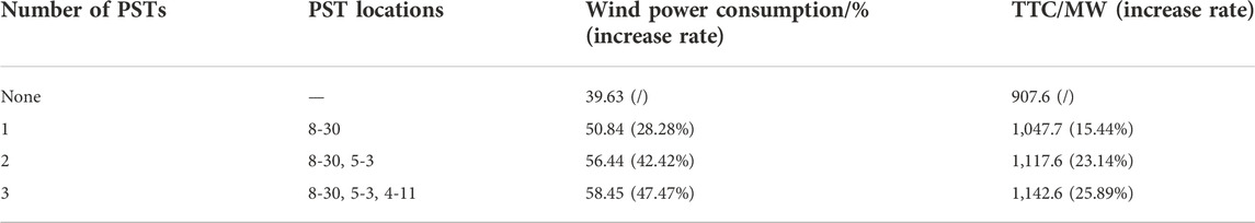
TABLE 6. IEEE 118-bus system results for various numbers of PSTs.

7.6 Computational issues

All the simulations are conducted on a test computer with an Intel(R) Xeon(R) W-2255 CPU @ 3.70 GHz and 128.00 GB of RAM.

To demonstrate the computation accuracy of the proposed method for solving TTC in Section 4.1.2, we selected a typical scenario to compare the computational results in three computational models.

Model 1. Use the sensitivity method in 3.1.2 without considering the correction by RPF.

Model 2. Use the result of the model1 as the initial point for RPF, and a subsequent correction is applied;

Model 3. Use RPF to calculate TTC directly.We consider the results obtained by RPF (model3) as the standard value and calculate the error of the results in model1 and model2. As observed in Table 7, the error of the results obtained by the sensitivity method is 1.28% and reduces to 0.03% after the correction by RPF.In terms of computational speed, the computation time of the sensitivity method is extremely short. The calculation time of RPF is very long for two main reasons. First, not only the generator output but also the phase shift angle need to be adjusted, so the computation work became greater compared to the conventional RPF. Second, small adjustment steps for each generator and phase shift angle have been set to get accurate results. The proposed method (model2) obtained more accurate results after the correction by RPF, and the computation time was greatly reduced compared to model3. Since the initial point obtained based on the sensitivity method is closer to the final point.

TABLE 7

TABLE 7. Computational comparison for different computational models.

8 Conclusion

This paper presents a dynamic programming method for optimal PST allocation, considering the evolution and wind power uncertainty of the grid. The proposed approach seeks to identify the optimal planning path of PST in multi-stage grid planning. To demonstrate the effectiveness of the proposed method, we compare the results under dynamic and static programming. The method is also applied to the model of a published manuscript, and the results prove the superiority of the proposed method. In addition, we present a calculation method for TTC of grids containing PST and wind power, for TTC is used as one of the optimization objectives.

The current research is aimed to optimize the planning path of PST by considering the evolution of the grid. However, the addition of other FACTS devices is not considered. Therefore, the main topics in future works are how the PST cooperates with other FATCS devices and the dynamic programming of multi-type FACTS.

Data availability statement

The original contributions presented in the study are included in the article/Supplementary Material, further inquiries can be directed to the corresponding author.

Author contributions

Investigation, ZL; methodology, KF and ZD; project administration, FL; supervision, CX; writing—original draft, KF; writing—review and editing, FL and ZD.

Funding

This research was funded by the Southern Power Grid Corporation’s Science and Technology Project (Project No. 037700KK52190015 (GDKJXM20198313)) and Key-Area Research and Development Program of Guangdong Province (2019B111109001).

Conflict of interest

FL and ZL was employed by The Grid Planning and Research Center of Guangdong Power Grid Corporation.

The remaining authors declare that the research was conducted in the absence of any commercial or financial relationships that could be construed as a potential conflict of interest.

The authors declare that this study received funding from the Southern Power Grid Corporation's Science and Technology Project. The funder had the following involvement in the study: Investigation, project administration, writing—review.

Publisher’s note

All claims expressed in this article are solely those of the authors and do not necessarily represent those of their affiliated organizations, or those of the publisher, the editors and the reviewers. Any product that may be evaluated in this article, or claim that may be made by its manufacturer, is not guaranteed or endorsed by the publisher.

Supplementary material

The Supplementary Material for this article can be found online at: https://www.frontiersin.org/articles/10.3389/fenrg.2022.1003315/full#supplementary-material

References

Bandara, H. M. M. T., Samarasinghe, D. P., Manchanayake, S. M. A. M., Perera, L. P. J., Kumaradasa, K. C., Pemadasa, N., and Samarasinghe, A.P. (2019). “Analyzing payment behaviors and introducing an optimal credit limit,” in Proceedings of the 2019 International Conference on Advancements in Computing (ICAC), Malabe, Sri Lanka, 05-07 December 2019 (IEEE), 68–72. doi:10.1109/ICAC49085.2019.9103404

CrossRef Full Text | Google Scholar

Baringo, L., and Conejo, A. J. (2013). Correlated wind-power production and electric load scenarios for investment decisions. Appl. Energy 101, 475–482. doi:10.1016/j.apenergy.2012.06.002

CrossRef Full Text | Google Scholar

Blumsack, S. (2006). Network topologies and transmission investment under electric-industry restructuring. Pittsburgh, PA, USA: Carnegie Mellon Univ. Thesis.

Google Scholar

Brilinskii, A. S., Badura, M. A., Evdokunin, G. A., Chudny, V. S., and Mingazov, R. I. (2020). “Phase-Shifting transformer application for dynamic stability enhancement of electric power stations generators,” in Proceedings of the 2020 IEEE Conference of Russian Young Researchers in Electrical and Electronic Engineering (EIConRus), St. Petersburg and Moscow, Russia, 27-30 January 2020 (IEEE), 1176–1178. doi:10.1109/EIConRus49466.2020.9039410

CrossRef Full Text | Google Scholar

Ding, T., Bo, R., Bie, Z., and Wang, X. (2017). Optimal selection of phase shifting transformer adjustment in optimal power flow. IEEE Trans. Power Syst. 32 (3), 2464–2465. doi:10.1109/TPWRS.2016.2600098

CrossRef Full Text | Google Scholar

Gerbex, S., Stephane, R., and Cherkaoui, A. J. (2001). Optimal location of Multi-Type FACTS devices in a power system by means of genetic algorithms. IEEE Trans. Power Syst. 16 (3), 537–544. doi:10.1109/59.932292

CrossRef Full Text | Google Scholar

Ghahremani, E., and Kamwa, I. (2013). Optimal placement of multiple-type FACTS devices to maximize power system loadability using a generic graphical user interface. IEEE Trans. Power Syst. 28 (2), 764–778. doi:10.1109/TPWRS.2012.2210253

CrossRef Full Text | Google Scholar

Hadzimuratovic, S., and Fickert, L. (2018). “Determination of critical factors for optimal positioning of Phase-Shift Transformers in interconnected systems,” in Proceedings of the 2018 19th International Scientific Conference on Electric Power Engineering (EPE), Brno, Czech Republic, 16-18 May 2018 (IEEE), 1–6. doi:10.1109/EPE.2018.8396033

CrossRef Full Text | Google Scholar

IEA (2017). Getting wind and sun onto the grid. AvaliableAt: https://www.iea.org/reports/getting-wind-and-solar-onto-the-grid.

Google Scholar

Ippolito, L., and Siano, P. (2004). Selection of optimal number and location of thyristor-controlled phase shifters using genetic based algorithms. IEE Proc. Gener. Transm. Distrib. 151 (5), 630–637. doi:10.1049/ip-gtd:20040800

CrossRef Full Text | Google Scholar

Kazemi, A., and Sharifi, R. (2006). “Optimal location of thyristor controlled phase shifter in restructured power systems by congestion management,” in Proceedings of the 2006 IEEE International Conference on Industrial Technology, Mumbai, India, 15-17 December 2006 (IEEE), 294–298. doi:10.1109/ICIT.2006.372211

CrossRef Full Text | Google Scholar

Li, F., Li, Z., Yu, M., Liu, R., Fu, K., and Du, Z. (2022a). Research on optimal location method of phase shifter based on improved PageRank algorithm. Guangdong Electr. Power 35 (5), 42–52. doi:10.3969/j.issn.1007-290X.2022.005.006

CrossRef Full Text | Google Scholar

Li, Z., Li, F., Liu, R., Yu, M., Chen, Z., Xie, Z., and Du, Z. (2022b). A Data-Driven genetic algorithm for power flow optimization in the power system with phase shifting transformer. Front. Energy Res. 9, 793686. doi:10.3389/fenrg.2021.793686

CrossRef Full Text | Google Scholar

Lima, F. G. M., Galiana, F. D., Kockar, I., and Munoz, J. (2003). Phase shifter placement in large-scale systems via mixed integer linear programming. IEEE Trans. Power Syst. 18 (3), 1029–1034. doi:10.1109/TPWRS.2003.814858

CrossRef Full Text | Google Scholar

Miranda, V., and Alves, R. (2014). “PAR/PST location and sizing in power grids with wind power uncertainty,” in Proceedings of the 2014 International Conference on Probabilistic Methods Applied to Power Systems (PMAPS), Durham, UK, 07-10 July 2014 (IEEE), 1–6. doi:10.1109/PMAPS.2014.6960679

CrossRef Full Text | Google Scholar

NEA (2022). NEA's first quarter of 2022 online press conferences. AvaliableAt: http://www.nea.gov.cn/2022-01/28/c_1310445390.htm.

Google Scholar

National Energy Renewable Laboratory (2019). Wind data-site 126685. AvaliableAt: https://egriddata.org/dataset/wind-data-site-126685.

Google Scholar

Preedavichit, P., and Srivastava, S. C. (1998). Optimal reactive power dispatch considering FACTS devices. Electr. Power Syst. Res. 46 (3), 251–257. doi:10.1016/S0378-7796(98)00075-3

CrossRef Full Text | Google Scholar

Sebaa, K., Bouhedda, M., Tlemçani, A., and Henini, N. (2014). Location and tuning of TCPSTs and SVCs based on optimal power flow and an improved cross-entropy approach. Int. J. Electr. Power & Energy Syst. 54, 536–545. doi:10.1016/j.ijepes.2013.08.002

CrossRef Full Text | Google Scholar

Tao, H., Xu, J., and Zou, W. (2013). Model conversion from BPA to PSCAD. Electr. Power Autom. Equip. 33 (8), 152–156. doi:10.3969/j.issn.1006-6047.2013.08.026

CrossRef Full Text | Google Scholar

Verboomen, J., Van Hertem, D., Schavemaker, P. H., Kling, W. L., and Belmans, R. (2008). Analytical approach to grid operation with phase shifting transformers. IEEE Trans. Power Syst. 23 (1), 41–46. doi:10.1109/TPWRS.2007.913197

CrossRef Full Text | Google Scholar

Wang, X., Wang, X., Sheng, H., and Lin, X. (2021). A Data-Driven sparse polynomial chaos expansion method to assess probabilistic total transfer capability for power systems with renewables. IEEE Trans. Power Syst. 36 (3), 2573–2583. doi:10.1109/TPWRS.2020.3034520

CrossRef Full Text | Google Scholar

Wu, Q. H., Lu, Z., Li, M. S., and Ji, T. Y. (2008). “Optimal placement of FACTS devices by a group search optimizer with multiple producer,” in Proceedings of the 2008 IEEE Congress on Evolutionary Computation (IEEE World Congress on Computational Intelligence), Hong Kong, China, 01-06 June 2008 (IEEE), 1033–1039. doi:10.1109/CEC.2008.4630923

CrossRef Full Text | Google Scholar

Yeo, J. H., Dehghanian, P., and Overbye, T. (2019). “Power flow consideration of impedance correction for phase shifting transformers,” in Proceedings of the 2019 IEEE Texas Power and Energy Conference (TPEC), College Station, TX, USA, 07-08 February 2019 (IEEE), 1–6. doi:10.1109/TPEC.2019.8662150

CrossRef Full Text | Google Scholar

Zhang, H., Yang, J., Ren, X., Wu, Q., Zhou, D., and Elahi, E. (2020). How to accommodate curtailed wind power: A comparative analysis between the us, Germany, India and China. Energy Strategy Rev. 32, 100538. doi:10.1016/j.esr.2020.100538

CrossRef Full Text | Google Scholar

Zhang, N., Zhu, X., and Liu, J. (2021). “Improving the consumption capacity of wind power in distributed network using a thyristor controlled phase shifting transformer,” in Proceedings of the 2021 3rd Asia Energy and Electrical Engineering Symposium (AEEES), Chengdu, China, 26-29 March 2021 (IEEE), 80–84. doi:10.1109/AEEES51875.2021.9403143

CrossRef Full Text | Google Scholar

Zhang, X., and Grijalva, S. (2013). “Multi-area ATC evaluation based on Kron reduction,” in Proceedings of the 2013 IEEE International Conference on Smart Energy Grid Engineering (SEGE), Oshawa, Canada, 28-30 August 2013 (IEEE), 1–6. doi:10.1109/SEGE.2013.6707921

CrossRef Full Text | Google Scholar

Zhang, X., Shi, D., Wang, Z., Yu, Z., Wang, X., Bian, D., and Tomsovic, K. (2017). “Bilevel optimization based transmission expansion planning considering phase shifting transformer),” in Proceedings of the 2017 North American Power Symposium (NAPS), Morgantown, WV, USA, 17-19 September 2017 (IEEE), 1–6. doi:10.1109/NAPS.2017.8107289

CrossRef Full Text | Google Scholar

Zhang, X., Shi, D., Wang, Z., Zeng, B., Wang, X., Tomsovic, K., and Jin, Y. (2018). Optimal allocation of series FACTS devices under high penetration of wind power within a market environment. IEEE Trans. Power Syst. 33 (6), 6206–6217. doi:10.1109/TPWRS.2018.2834502

CrossRef Full Text | Google Scholar

Ziaee, O., and Choobineh, F. (2017). Optimal Location-Allocation of TCSCs and transmission switch placement under high penetration of wind power. IEEE Trans. Power Syst. 32 (4), 3006–3014. doi:10.1109/TPWRS.2016.2628053

CrossRef Full Text | Google Scholar