 Zhao Yao1,2
 Yingshun Li2*
- 1Army Academy of Armored Forces, Changchun, China
- 2Dalian University of Technology, Dalian, China
A novel echo state network (ESN), referred to as a fuzzy-weighted echo state network (FWESN), is proposed by using the structural information of data sets to improve the performance of the classical ESN. The information is incorporated into the classical ESN via the concept of Takagi–Sugeno (TS) models/rules. We employ the fuzzy c-mean clustering method to extract the information based on the given data set. The antecedent part of the TS model is determined by the information. Then, we obtain new fuzzy rules by replacing the affine models in the consequent part of each TS rule with a classical ESN. Consequently, the output of the proposed FWESN is calculated through inferring these new fuzzy rules by a fuzzy-weighted mechanism. The corresponding reservoir is consisted of the sub-reservoirs of the new fuzzy rules. Furthermore, we prove that the FWESN has an echo state property by setting the largest spectrum radium of all the internal weight matrices in the sub-reservoirs less than one. Finally, a nonlinear dynamic system and five nonlinear time series are employed to validate the FWESN.
1 Introduction
1.1 Summary of the Echo State Network
The recurrent network model describes the change process of the states of research object with time and space. Since the complexity of the problem increases and the computing power enhances, various recurrent networks have been successfully applied to different application fields, such as echo state networks in time series prediction (Jaeger and Haas, 2004), Boolean networks in games (Le et al., 2021; Le et al., 2020), and optimal control (Chen et al., 2019; Toyoda and Wu, 2021; Wu et al., 2021).
Echo state networks (ESNs) are a special case of recurrent neural networks (RNNs) proposed by Jaeger and Haas (2004). Unlike the traditional RNN, the recurrent layer of ESN uses a large number of neurons, and the connection weights between neurons are randomly generated and sparse. In an ESN, the recurrent layer is called a reservoir. The input signals drive the reservoir, and the trainable output neurons combine the output of the reservoir to generate task-special temporal patterns. This new RNN paradigm is referred to as reservoir computing. Similar to ESNs, liquid state machines (Maass et al., 2002), temporal recurrent neural networks (Steil, 2006), and decorrectation–backpropagation learning (LukošAevicius and Jaeger, 2009), and convolution and deep echo state networks (Ma et al., 2021; Wang et al., 2021) are all the instances of reservoir computing. The difference between ESNs and them is that the former employs analog neurons. The problem of traditional RNN is the lack of an effective supervised training algorithm. This problem is largely overcome by ESNs since only output weights are trained. ESNs have been successfully applied in a wide range of temporal tasks (Jaeger and Haas, 2004; Holzmann and Hauser, 2010; Song and Feng, 2010; Babinec and Pospichal, 2012; Xu et al., 2019; Yang and Zhao, 2020), especially in the prediction of nonlinear chaotic time series (Jaeger and Haas, 2004; Wang et al., 2021).
1.2 Summary of the Related Work and Motivation
The random and sparse connection weights between neurons in the reservoir bring much convenience for ESN applications. However, just simply creating at random is unsatisfactory for a specific modeling task (LukošAevicius and Jaeger, 2009). Recently, one of main streams for ESN research has been focused on developing a suitable reservoir to improve its performance (Jaeger, 2007; Holzmann and Hauser, 2010; Song and Feng, 2010; Babinec and Pospichal, 2012; Sheng et al., 2012). The fact shows that a specific architectural variant of the standard ESN leads to better results than that of a naive random creation. For examples, a new ESN with arbitrary infinite impulse response filter neurons is proposed for the task of learning multiple attractors or signal with different time scales. Then, the trainable delays in the synapse connection of output neurons are added to improve the memory capacity of ESNs (Holzmann and Hauser, 2010). Inspired by the simulation results of some nonlinear time series prediction, a complex ESN is proposed, in which the connection process of its reservoir is determined by five growth factors (Song and Feng, 2010). A complex prediction system is created by combining the local expert ESN with different memory length for solving the troubles of ESN with fixed memory length in applications (Babinec and Pospichal, 2012). A hierarchical architecture of ESN is presented for multi-scale time series. Its core ingredient of each layer is an ESN. This architecture as a whole is trained by a stochastic error gradient descent (Jaeger, 2007). An improved ESN is proposed to predict the noisy nonlinear time series, in which the uncertainties from internal states and outputs are meanwhile considered in accordance with the industrial practice (Sheng et al., 2012).
Note that uncertain information, noises, and structure information often exist in the systems (Liu and Xue, 2012; Shen et al., 2020; Shen and Raksincharoensak, 2021a,b). Thus, an extensive work has been carried out on designing a specific reservoir for a given modeling task as mentioned previously. However, the structure information for the input/output data is ignored when the reservoir is designed or revised. In fact, for many temporal tasks and pattern recognition problems, the data sets appear in homogenous groups, and this structural information can be exploited to facilitate the training process, so that the prediction accuracy can be further improved (Wang et al., 2007; Liu and Xue, 2012). Thus, it becomes a necessary requirement to consider the effects of data structure information on the ESN and then to design a suitable reservoir for a specific modeling task.
1.3 Main Idea and Contributions
This study aims at constructing a new type of ESN, referred to as a fuzzy-weighted echo state network (FWESN). The FWESN is able to incorporate the structural information of data sets into the classical ESN via the TS model. Actually, the FWESN can be regarded as a certain ESN, in which the output is calculated by a fuzzy-weighted mechanism, and the corresponding reservoir consists of sub-reservoirs corresponding to TS rules. Similar to the ESN, the echo state property for the FWESN is obtained when all weighted matrices of sub-reservoirs satisfy that their spectrums are less than one.
The contribution of this article lies in the following aspects: first, the structural information of the data set is incorporated into the classical ESN to enhance its performance in applications.
Second, the structure of FWESN is parallel, which is distinguished from the hierarchical architecture of ESN. The FWESN is trained efficiently by a linear regression problem, which is the same as the training algorithms of the ESN and TS model. Thus, the FWESN avoids the problem of vanishing gradients, as the hierarchical ESN, deep feedforward neural networks, and fully trained recurrent neural networks based on gradient-descent methods.
The remaining article is structured as follows: preliminaries are given in Section 2. The architecture, echo state property, and training algorithm of FWESN are discussed in Section 3. Experiments are performed by comparing FWESN with the ESN and TS model in Section 4. Finally, conclusions are drawn in Section 5.
2 Preliminaries
In this section, we give a brief introduction to typical ESNs and TS models. A more thorough treatments concerning them can be referred to Takagi and Sugeno (1985), Jaeger and Haas (2004), and Holzmann and Hauser (2010).
2.1 Echo State Networks
An ESN can be represented by state update and output equations. We formulate the ESN as shown in Figure 1.
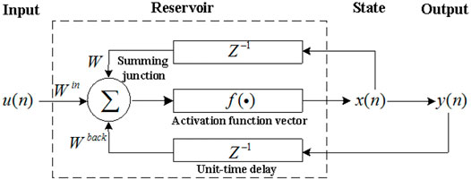
FIGURE 1. Architecture of the echo state network.
The activation of internal units in a reservoir is updated according to the following equations:.
Here,
where
and
is the output weight matrix.
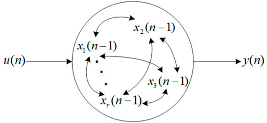
FIGURE 2. Full connection of internal units in a reservoir.
There are several notions of stability relevant to ESNs, where the echo state property is the most basic stability property (Jaeger and Haas, 2004).
Let
to denote the network state that results from an iterated application of Eq. 1. If the input sequence
Definition 1: Assume that the inputs are drawn from a compact input space
The condition of Def. 1 is hard to check in practice. Fortunately, a sufficient condition is given in Jaeger and Haas (2004), which is easily checked.
Proposition 1: Assume a sigmoid network with unit output functions fi = tanh. Let the weight matrix W satisfy σmax = ∧ < 1, where σmax is the largest singular value of W. Then,
2.2 Takagi–Sugeno Models
Among various fuzzy modeling themes, the TS model (Takagi and Sugeno, 1985) has been one of the most popular modeling frameworks. A general TS model employs an affine model in the consequent part for every fuzzy rule. We formulate the TS model as shown in Figure 3.
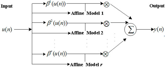
FIGURE 3. Architecture of the TS model.
A TS model can be represented with r fuzzy rules and each fuzzy rule has the following form:
where
is the output from the ith fuzzy rule, where
Given an input u(n), the final output of the fuzzy system is inferred as follows:
where
3 Fuzzy-Weighted Echo State Networks
In this section, we propose a new framework based on the ESN and TS model, which is referred to as a fuzzy-weighted echo state network (FWESN). We further prove that an FWESN has the echo state property. Finally, we discuss the training algorithm of FWESN.
3.1 Architecture of Fuzzy-Weighted Echo State Networks
FWESNs are designed by taking advantage of TS models to improve ESN (1). The basic idea is to replace the affine model of each fuzzy rule (4) with ESN (1). FWESN is formulated as shown in Figure 4.
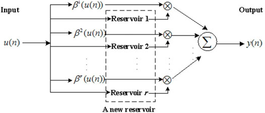
FIGURE 4. Architecture of FWESN.
The FWESN can be represented by the fuzzy rules as follows:
where y(n) is the output for the ith fuzzy rule (6). y(n) is determined by the following state update equations:
Here,
Let
By Eq. 6, a new reservoir can be reformulated, where the state update equations are written as
Additionally, the same shorthand is used for the FWESN and ESN. Thus, from Eqs. 3, 9, it follows that
which denotes the network state resulting from an iterated applications. For an FWESN without feedback, Eq. 10 is simplified as
For clarity, we use (β, Win, W, Wback, Wout) to denote an FWESN, where
3.2 Discussion on Several Special Cases for Fuzzy-Weighted Echo State Networks
Case 1: From the architecture of FWESN, the classical ESN can be regarded as a special case of FWESN. That is, let r = 1 and
in Eq. 6. Then, the final output of FWESN (8) is rewritten as
The corresponding update Eq.7 is expressed as
which is the same as ESN (1).
Case 2: The TS model (4) can be regarded as a special case of FWESN (6). That is, let fi = (1,0,…,0)T in Eq. 6. It follows that
and
Let
Then, we have the output of the ith fuzzy rule (6) as follows:
It is obvious that the fuzzy rule (6) has the same form as that of the fuzzy rule (4) based on the aforementioned conditions. Thus, the FWESN degrades into the TS model (4).
3.3 Echo State Property of Fuzzy-Weighted Echo State Networks
In this section, we will prove that the FWESN has the echo state property for the case of the network without output feedback. Similar to Proposition 1, we give a sufficient condition for the echo state property of the FWESN.
Proposition 2: Let
This implies the echo states for all inputs
Proof: Considering W = diag (W1, W2, …, Wr) and σ(Wi) < 1, we have
Here, λmax (⋅) is the largest absolute value of an eigenvector of matrix. For two different states X(n) and
For
where
That is, the Lipschitz condition obviously results in echo states for the FWESN.
Remark 1: From the proof of Proposition 2, we select that the updated Eq. 1 is a special form based on the conditions σ(Wi) < 1 for i = 1, 2, …, r.
3.4 Training Algorithm of Fuzzy-Weighted Echo State Networks
We state the training algorithm of FWESN based on the given training input/output pairs (u(n), z(n)) (n = 0, 1, 2, …, k). First, we employ a subtractive clustering approach (Bezdek, 1981) to determine the membership grade
The procedure of the proposed training algorithm is described by four steps as follows:
Step 1 Calculate βi (u(n)) (i = 1, 2, …, r) in Eq. 8 by the fuzzy c-mean clustering approach.
Step 2 Procure the untrained network
1) Suppose the dimension of the state vector is N for r reservoirs corresponding to r fuzzy rules (5).
2) Initiate i = 1.
3) Randomly generate an input weight matrix Win, an output backpropogation weight matrix Wback, and a matrix
4) Let
5) If i > r, end. Else go to Step 3.
Step 3 Sample network training dynamics for each fuzzy rule (4).
1) Let i = 1. Initial the state of the untrained network
2) Drive the network
3) For each time equal or larger than an initial washout time
4) i = i + 1, if i > r, end; else go to Step 2.
Step 4 Calculate the output weights.
1) Let
Collect βi (u(n))Si(n) as a state matrix S for
2) By the least square method, the output weight Wout is calculated by Wout = (SST)YST.
Remark 2: By Step 2, we obtain untrained networks
4 Experiments
We have performed some experiments to validate the FWESN in this study. We have shown that the FWESN has better performance than the ESN owing to the incorporation of structural information of data sets. The following terms are used in the experiments:
Data sets: A nonlinear dynamic system (Juang, 2002) and five nonlinear time series, i.e., Mackey-Class, Lorenz, ESTSP08(A), ESTSP08(B), and ESTSP08(C), are used in the experiments. Here, the nonlinear dynamic system is
where
yp(k) and u(k) are the output and input, respectively. In the experiment, (u(k), yp (k − 1)) and yp(k) are the inputs and outputs of algorithms, respectively. The generate method of samples are the same with that in Juang (2002).
Algorithms: Three algorithms, i.e., FWESN, ESN, and TS model, are used in the experiments. The neurons in the form of hyperbolic tangent functions are used for the ESN and FWESN.
Parameters: r is the number of fuzzy rules. The main parameters of the reservoir are the scale of the reservoir N, the sparseness of the reservoir SD, the spectrum radium of the internal weight matrices in the reservoir SR, the input-unit scale IS, and shifting IT. In the experiments, FWESN and ESN use the same scale N, where N = rNi for FWESN, where Ni represents the scales of sub-reservoirs corresponding to Eq. 6, where i = 1, 2, …, r. Moreover, N1 = N2 = … = Nr. Additionally, SR, IS, IT, and SD in all sub-reservoirs of FWESN and the reservoir of ESN are the same. Thus, from Eq. 13, it follows that the spectra radius of W in Eq. 9) is the same as that in Eq. 1. Finally for the FWESN and TS model, both the parameters in the antecedent part and the total number of fuzzy rules are the same.
Performance Indices: We choose the training and test errors as the performance indices. All the errors refer to the mean square errors in the experiment.
Experimental Results: The simulation results are summarized in Table 1.
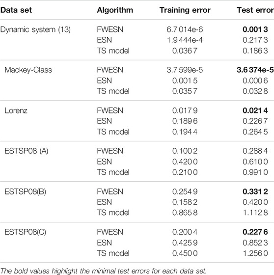
TABLE 1. Experiment results for FWESN, ESN, and TS model.
From Table 1, the FWESN achieves better performance than the ESN and TS model under same conditions. The bold values in Table 1 highlight the minimal test errors for each data set. For example, by the FWESN and dynamic system Eq. 1, the training and test errors are, respectively, 6.7 014e-6 and 0.001 3, which are far less than the errors based on the ESN and TS model. Thus, the learning ability and generalization ability are obviously better than the ESN and TS model. The similar results are obtained for the five nonlinear time series from Figure 5. On the one hand, the test errors of FWESN are less than those of ESN. The scale of FWESN and ESN are the same. The comparison indicates that the FWESN enhances the performance of ESN since we incorporate the structural information of the data sets into the ESN via the form of fuzzy weight. Additionally, the FWESN has better prediction ability, especially for nonlinear time series, than the TS model while their total number of fuzzy rules and the antecedent part of each fuzzy rule are the same.
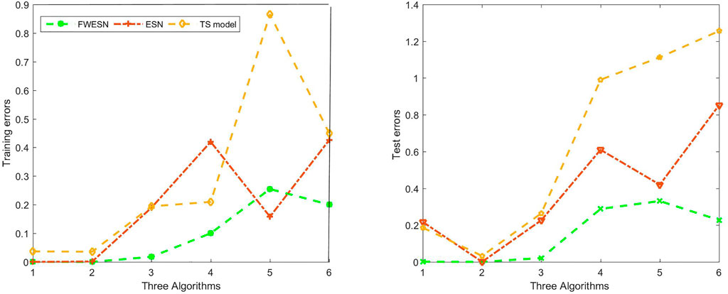
FIGURE 5. Training and test errors for FWESN, ESN, and TS model.
5 Conclusion
In this work, a novel framework with the advantages of the ESN and TS model is proposed. As a generalization of both ESN and TS model, the ESN and TS model are improved and extended. Similar to the classical ESN, we prove that if the largest spectrum radium of the internal unit weight matrix is less than one, the FWESN has the echo state property. The FWESN shows higher accuracy than the TS model and ESN. For future work, we plan to continuously investigate the underlying theory problem of FWESN, such as the tighter stability conditions and approximation capability to a dynamical system or static function. We attempt to more different applications, for e.g., remaining useful life predictions. Additionally, we will consider hardware, for e.g., field-programmable gate array (FPGA) and implementation of FWESN oriented to real-time applications. Actually, with the development of computing power and access to big data, the convolutional neural networks are very popular owing to their obvious advantages. Thus, one further research will focus on the deep ESN based on the structural information of big data. We believe that some better results will be obtained through incorporating FWESN and deep-learning methods.
Data Availability Statement
The raw data supporting the conclusions of this article will be made available by the authors, without undue reservation.
Author Contributions
ZY contributed to the architecture, property, and training algorithm of fuzzy-weighted echo state networks. YL drafted the manuscript and contributed to the experiments and conclusions. All authors agree to be accountable for the content of the work.
Funding
This work was financially supported by the China Postdoctoral Science Foundation (Grant No. 2020M670785).
Conflict of Interest
The authors declare that the research was conducted in the absence of any commercial or financial relationships that could be construed as a potential conflict of interest.
Publisher’s Note
All claims expressed in this article are solely those of the authors and do not necessarily represent those of their affiliated organizations, or those of the publisher, the editors, and the reviewers. Any product that may be evaluated in this article, or claim that may be made by its manufacturer, is not guaranteed or endorsed by the publisher.
References
Babinec, S., and Pospichal, J. (2012). Modular echo State Neural Networks in Time Series Prediction. Comput. Inform. 30, 321–334.
Bezdek, J. C. (1981). Pattern Recognition with Fuzzy Objective Function Algorithms. New YorkBoston, MA): Springer.
Chen, S., Wu, Y., Macauley, M., and Sun, X.-M. (2019). Monostability and Bistability of Boolean Networks Using Semitensor Products. IEEE Trans. Control. Netw. Syst. 6, 1379–1390. doi:10.1109/TCNS.2018.2889015
Chia-Feng Juang, C.-F. (2002). A TSK-type Recurrent Fuzzy Network for Dynamic Systems Processing by Neural Network and Genetic Algorithms. IEEE Trans. Fuzzy Syst. 10, 155–170. doi:10.1109/91.995118
Holzmann, G., and Hauser, H. (2010). Echo State Networks with Filter Neurons and a Delay∑ Readout. Neural Networks 23, 244–256. doi:10.1016/j.neunet.2009.07.004
Jaeger, H. (2007). Discovering Multiscale Dynamical Features with Hierarchical echo State Networks. (Bremen: Jacos University Breme).
Jaeger, H., and Haas, H. (2004). Harnessing Nonlinearity: Predicting Chaotic Systems and Saving Energy in Wireless Communication. Science 304, 78–80. doi:10.1126/science.1091277
Le, S., Wu, Y., Guo, Y., and Vecchio, C. D. (2021). Game Theoretic Approach for a Service Function Chain Routing in NFV with Coupled Constraints. IEEE Trans. Circuits Syst. 68, 3557–3561. doi:10.1109/TCSII.2021.3070025
Le, S., Wu, Y., and Toyoda, M. (2020). A Congestion Game Framework for Service Chain Composition in NFV with Function Benefit. Inf. Sci. 514, 512–522. doi:10.1016/j.ins.2019.11.015
Liu, F., and Xue, X. (2012). Design of Natural Classification Kernels Using Prior Knowledge. IEEE Trans. Fuzzy Syst. 20, 135–152. doi:10.1109/TFUZZ.2011.2170428
Lukoševičius, M., and Jaeger, H. (2009). Reservoir Computing Approaches to Recurrent Neural Network Training. Comp. Sci. Rev. 3, 127–149. doi:10.1016/j.cosrev.2009.03.005
Ma, Q., Chen, E., Lin, Z., Yan, J., Yu, Z., and Ng, W. W. Y. (2021). Convolutional Multitimescale echo State Network. IEEE Trans. Cybern. 51, 1613–1625. doi:10.1109/TCYB.2019.2919648
Maass, W., Natschläger, T., and Markram, H. (2002). Real-time Computing without Stable States: A New Framework for Neural Computation Based on Perturbations. Neural Comput. 14, 2531–2560. doi:10.1162/089976602760407955
Shen, X., and Raksincharoensak, P. (2021a). Pedestrian-aware Statistical Risk Assessment. IEEE Trans. Intell. Transport. Syst., 1, 9. doi:10.1109/TITS.2021.3074522
Shen, X., and Raksincharoensak, P. (2021b). Statistical Models of Near-Accident Event and Pedestrian Behavior at Non-signalized Intersections. J. Appl. Stat., 1, 21. doi:10.1080/02664763.2021.1962263
Shen, X., Zhang, X., and Raksincharoensak, P. (2020). Probabilistic Bounds on Vehicle Trajectory Prediction Using Scenario Approach. IFAC-PapersOnLine 53, 2385–2390. doi:10.1016/j.ifacol.2020.12.038
Sheng, C., Zhao, J., Liu, Y., and Wang, W. (2012). Prediction for Noisy Nonlinear Time Series by echo State Network Based on Dual Estimation. Neurocomputing 82, 186–195. doi:10.1016/j.neucom.2011.11.021
Song, Q., and Feng, Z. (2010). Effects of Connectivity Structure of Complex echo State Network on its Prediction Performance for Nonlinear Time Series. Neurocomputing 73, 2177–2185. doi:10.1016/j.neucom.2010.01.015
Steil, J. J. (2006). Online Stability of Backpropagation-Decorrelation Recurrent Learning. Neurocomputing 69, 642–650. doi:10.1016/j.neucom.2005.12.012
Takagi, T., and Sugeno, M. (1985). Fuzzy Identification of Systems and its Applications to Modeling and Control. IEEE Trans. Syst. Man. Cybern. SMC-15, 116–132. doi:10.1109/TSMC.1985.6313399
Toyoda, M., and Wu, Y. (2021). Mayer-type Optimal Control of Probabilistic Boolean Control Network with Uncertain Selection Probabilities. IEEE Trans. Cybern. 51, 3079–3092. doi:10.1109/TCYB.2019.2954849
Wang, D., Yeung, D. S., and Tsang, E. C. C. (2007). Weighted Mahalanobis Distance Kernels for Support Vector Machines. IEEE Trans. Neural Netw. 18, 1453–1462. doi:10.1109/TNN.2007.895909
Wang, Z., Yao, X., Huang, Z., and Liu, L. (2021). Deep echo State Network with Multiple Adaptive Reservoirs for Time Series Prediction. IEEE Trans. Cogn. Dev. Syst. 13, 693–704. doi:10.1109/TCDS.2021.3062177
Wu, Y., Guo, Y., and Toyoda, M. (2021). Policy Iteration Approach to the Infinite Horizon Average Optimal Control of Probabilistic Boolean Networks. IEEE Trans. Neural Netw. Learn. Syst. 32, 2910–2924. doi:10.1109/TNNLS.2020.3008960
Xu, M., Yang, Y., Han, M., Qiu, T., and Lin, H. (2019). Spatio-temporal Interpolated echo State Network for Meteorological Series Prediction. IEEE Trans. Neural Netw. Learn. Syst. 30, 1621–1634. doi:10.1109/TNNLS.2018.2869131
Keywords: echo state network, Takagi–Sugeno model, fuzzy, reservoir, time series prediction
Citation: Yao Z and Li Y (2022) Fuzzy-Weighted Echo State Networks. Front. Energy Res. 9:825526. doi: 10.3389/fenrg.2021.825526
Received: 30 November 2021; Accepted: 28 December 2021;
Published: 17 March 2022.
Edited by:
Xun Shen, Tokyo Institute of Technology, JapanReviewed by:
Datong Liu, Harbin Institute of Technology, ChinaCopyright © 2022 Yao and Li. This is an open-access article distributed under the terms of the Creative Commons Attribution License (CC BY). The use, distribution or reproduction in other forums is permitted, provided the original author(s) and the copyright owner(s) are credited and that the original publication in this journal is cited, in accordance with accepted academic practice. No use, distribution or reproduction is permitted which does not comply with these terms.
*Correspondence: Yingshun Li, bGVleXNAZGx1dC5lZHUuY24=