The Leading-Edge Structure Based on Geometric Bionics Affects the Transient Cavitating Flow and Vortex Evolution of Hydrofoils

A hydrofoil is a fundamental structure in fluid machinery, and it is widely applied to the fields of propellers, blades of axial flow pumps and underwater machinery. To reveal that the geometric structure of the leading-edge of a hydrofoil is the mechanism that affects the transient cavitating flow, we regard the three fish-type leading-edge structures of mackerel, sturgeon and small yellow croaker as the research objects and use high-precision non-contact 3D scanners to establish three bionic hydrofoils (Mac./Stu./Cro.). We use large eddy simulation to simulate the transient cavitating flow of hydrofoils numerically and compare and analyze their lift–drag characteristics, the transient behavior of unsteady cavitation and the vortex evolution. The numerical simulation results are in good agreement with the experimental results. The warping of leading-edge structure will cause a change in lift–drag characteristics, and the Cro. hydrofoil has a good lift-to-drag ratio. When the leading-edge structure is tilted upward (Cro. hydrofoil), the position of the attached cavity will move forward, which will accelerate the cavitation evolution and improve the velocity fluctuation of the trailing edge. When the leading-edge structure is tilted downward (Stu. hydrofoil), the change in the vortex stretching and dilatation terms will be complex, and the influence area of the vortex will widen.

Introduction

Cavitation is a typical vapor-liquid flow, and mass transmission is determined using the bypass pressure and the local vaporisation pressure of the fluid. The fluid bypassing a hydrofoil will generate lift. In accordance with this principle, hydrofoils are widely used in the field of hydraulic machinery. However, cavitating flow is prone to occur in the application process, and a long-term operation under cavitation will cause cavitation erosion, which will seriously affect the performance of hydraulic machinery. In-depth research has found that the leading-edge geometry of a hydrofoil is the key factor affecting the aerofoil cavitating flow (Arabnejad et al., 2019; Liu and Tan, 2020; Garg et al., 2019). Most aerofoils used in hydraulic machinery are still based on aerodynamics. The fluid flow state will inevitably be changed by the difference in physical properties, such as density and viscosity, between air and water and other liquid fluids, thereby affecting the cavitation performance of hydraulic machinery. Therefore, changing the structure of the leading-edge of a hydrofoil and developing a new type of aerofoil suitable for hydraulic machinery are particularly important. A large number of fishes are living in oceans and freshwater lakes. These fishes have excellent hydraulic properties and provide basic materials for changing the structure of the leading-edge of a hydrofoil.

Researchers have conducted considerable basic research on the cavitating flow of different hydrofoils. For example, Zhang et al. (2020) used numerical simulation to study the hydrodynamic characteristics of the Clark-y hydrofoil and found that the cavitation of the leading-edge promotes the formation of a counterclockwise vortex at the trailing edge and weakens the fluctuation in hydrodynamic load. Rajaram and Srikanth (2020) optimised the geometry of a basic hydrofoil to obtain a superior hydrofoil under specific flow conditions. Marimon et al. (2018) evaluated a simplified hydrofoil geometry and used a performance prediction method for flexible foils to prove that distortion will reduce the effective angle of attack by approximately 30% and substantially reduce the lift and drag of the hydrofoil at high flow rates. Antoine et al. (2009) analysed the structural characteristics of a deformable hydrofoil in a forced pitching motion and showed that structural changes are closely related to the phenomenon of fluid mechanics. Fujii et al. (2007) also studied the influence of hydrofoil geometry on cavitation dynamic characteristics, and found that the change of hydrofoil geometry only affects the oscillation intensity of some cavities. Custodio et al. (2018) defined different hydrofoil leading-edge structures to study the cavitation and hydrodynamic characteristics of hydrofoils. The results showed that the cavitation of the hydrofoil with a large amplitude is mainly confined to the area behind a convex groove, whereas the hydrofoil with a flat leading-edge and small amplitude shows flaky cavitation in the whole span direction. Oller and Nallim (2016) designed the geometric structure of a hydrofoil blade by using an appropriate aerofoil shape to check its hydrodynamic characteristics and determine the streamline velocity and pressure field. Amini et al. (2019) used an ellipse as the contour of the hydrofoil and studied its suppression effect on tip vortex cavitation by bending the hydrofoil. For the hydrofoil (10%-bent 90 degrees-downward), the tangential velocity of the leading-edge vortex is improved. Zhou et al. (2016) studied the effect of the wingtip clearance on the flow characteristics of the hydrofoil. The sharp-tip foil has a small amount of vortex leakage, and the tip separation vortex makes the gap cavitation more serious. Recent studies have confirmed that the hydrodynamic and lift–drag characteristics of a blade can be significantly improved by changing the shape of the leading-edge of a hydrofoil.

Bionics is a comprehensive cross-discipline that applies the laws and mechanisms discovered in the biological world to the engineering application field to solve problems. Many methods for solving problems have been found using biological geometry, physiological functions or life processes in engineering practice (Hong et al., 2009). Huang et al. (2020) designed three new dolphin-type hydrofoils based on the contour curve of a dolphin and compared them with NACA0018 aerofoils. They found that the hydrofoils have the best lift–drag characteristics when the deflection angle is 24°. You et al. (2020) designed two bionic tools based on the surface structure of a dung beetle head, which effectively reduced the main cutting force of the tools and the average friction coefficient of the chip interface. Liu and Liu (2014) constructed a bionic hydrofoil based on the geometric characteristics of an owl, which effectively improved the lift and drag characteristics of the hydrofoil and revealed the characteristics of the sound source. Xue et al. (2016) regarded fish as imitation organisms and designed a fin–peduncle propulsion mechanism in accordance with their shape, which improved the propulsion efficiency of hydrofoil propellers. In the above research report, when obtaining the surface information of an organism, acquiring an accurate bionic physical model through curve-fitting technology is a critical step. In the aspect of bionic hydrofoil design, the Hicks–Henne shape function method with a strong hydrofoil shape control capability (Hicks and Henne, 1978), the CST aerofoil parameterisation method with a large design space description (Kulfan, 2008) and the spline parameterisation method using a non-uniform rational B-spline (NURBS) curve (Masters et al., 2017) to describe aerofoils are the commonly used modeling methods. These methods can provide theoretical support for this paper.

With the development of CFD technology, the numerical simulation technology based on large eddy simulation (LES) has been widely used in capturing complex cavitating flows and vortex evolution. Wang et al. (2019) simulated the cavitating flow of liquid nitrogen on a hydrofoil on the basis of a homogeneous mixture model with LES and found that the strong re-entrant jet initiated in the cavity tail is the main reason causing the cavity shedding. Huang et al. (2010) proposed a cavitating flow calculation model based on density correction to calculate the cavitating flow of a hydrofoil and found that this model has a significant improvement in the numerical calculation results of cavitating flow. Zhang et al. (2015) studied the unstable cavitation desorption of the Clark-y hydrofoil by increasing the maximum density ratio, which improved the accuracy of numerical simulation. Li et al. (2016) used the LES method to simulate the transient spatiotemporal flow of the Clark-y hydrofoil, which provided an effective numerical simulation framework for the study of cavitating flow. Ji et al. (2015) used the LES method to numerically simulate the cavitating flow around the NACA66 hydrofoil to study the evolution of cavitation. Sun et al. (2020) used the Schnerr–Sauer cavitation model to simulate hydrofoil cavitation and used the LES method to calculate an unsteady natural ventilation cavitation flow. Huang et al. (2017) proposed an improved partially averaged Navier–Stokes turbulence model to study the transient cavitation turbulence of the Clark-y hydrofoil. Kim and Lee (2015) used LES to study the cloud cavitation behaviour of the Clark-y hydrofoil under different slip conditions.

In summary, the research on hydrofoil hydrodynamics has mainly focused on the lift–drag characteristics and cavitating flow of existing aerofoils (NACA, Clark-y series hydrofoils). However, on the basis of different fishes, the basic research on using geometric bionic principles to change the geometric structure of the traditional hydrofoil leading-edge and analyse the 3D vortex structure and cavitating flow evolution is inadequately deep. Therefore, we select three fishes (mackerel/sturgeon/small yellow croaker) with evident leading-edge differences as the research objects to construct a bionic hydrofoil physical model. The lift–drag characteristics, vortex evolution and cavitating flow evolution under different schemes are compared and analysed through the combination of LES and typical hydrofoil model experiments to reveal the mechanism of the change in the hydrofoil leading-edge structure in transient cavitating flow. This study provides a reference for the subsequent optimisation design of hydraulic machinery blades.

Numerical Method and Setup

Establishment of the Physical Model of Bionic Hydrofoils

Through measurement, we found that mackerel, sturgeon, and small yellow croaker have different leading edge structures. We take these three kinds of fish as the research objects, as shown in Figure 1A. Ten fish are selected for each type of fish, and the average value is collected several times to avoid the error caused by the different body sizes of fish. High-precision non-contact 3D scanners are used to perform 3D reverse engineering modeling of all types of fish surface functional surfaces, and Geomagic Design X software is used to reverse the process of obtaining point cloud data to acquire a 3D physical model of fish, as shown in Figure 1B. The geometric profile curves of different hydrofoils are obtained and combined with the contours of the Clark-y hydrofoil via the NURBS curve-fitting technology. Four hydrofoils with different leading-edge structures are obtained, as shown in Figure 1C.

FIGURE 1

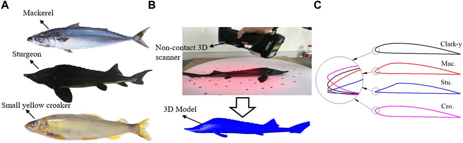
FIGURE 1. Physical model construction of bionic hydrofoils. (A) Three types of fishes. (B) 3D reverse engineerin. (C) contour curves of four hydrofoils.

Simulation Setup

In this study, the commercial software FLUENT is used for numerical simulation. LES is used to calculate the transient cavitating flow of the above four hydrofoils numerically, and the setting of the calculation domain is shown in Figure 2A (Hu et al., 2018). The chord length of all hydrofoils is set to C = 70 mm, the angle of attack is 8°, the calculated area length is 10 C, the height is 2.7 C, and the width is 0.5 C. The distance from the hydrofoils to the inlet is 4 C, and the distance to the bottom is 1.4 C. The finite volume method is used to discretize the governing equation, and the diffusion term of the equation is in central difference format. The equations are solved using the separation and semi-implicit pressure coupling algorithm. The inlet is set to imposed velocity, the flow rate is 10 m/s, the outlet is set as fixed static pressure, and the pressure is 43,540 Pa. It can be obtained that the cavitation number is 0.8 and the Reynolds number is 700,000. The hydrofoil walls adopt the no-slip boundary condition, the upper and lower walls are set as the free slip walls, and the sidewall boundary is arranged as a periodicity interface. The time step is set to 0.1 ms, and the number of calculation steps is set to 6,000 steps (Zhang et al., 2017).

FIGURE 2

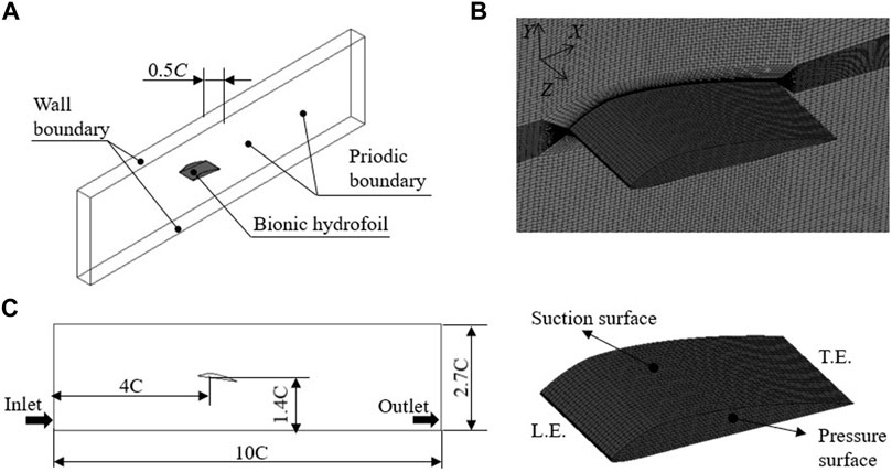
FIGURE 2. Computational domain and grids. (A) Computational area. (B) 3D mesh. (C) hydrofoil.

For LES, the basic governing equations of mass conservation and momentum conservation are as follows:

$\frac{\partial {\rho }_m}{\partial t}+\frac{\partial \left({\rho }_m{u}_i\right)}{\partial x_i}=0(1)$

$\frac{\partial \left({\rho }_m{u}_i\right)}{\partial t}+\frac{\partial \left({\rho }_m{u}_i{u}_j\right)}{\partial x_j}=-\frac{\partial p}{\partial x_i}+\frac{\partial }{\partial x_j}\left(\mu \frac{\partial u_i}{\partial x_j}\right)(2)$

Among them, $p$ represents the pressure, and $u_i$ and $u_j$ represent the velocity components on $i$ and $j$ respectively. $\mu$ is the laminar viscosity of the mixture, ${\rho }_m$ is the density of the mixture, which is defined as follows:

$\mu ={\alpha }_v{\mu }_v+\left(1-{\alpha }_v\right){\mu }_l(3)$

${\rho }_m={\alpha }_v{\mu }_v+\left(1-{\alpha }_v\right){\mu }_l(4)$

After filtering the above equation, the large eddy equation is obtained:

$\frac{\partial p}{\partial t}+\frac{\partial \left({\rho }_m{\overline{u}}_i\right)}{\partial x_i}=0(5)$

$\frac{\partial \left({\rho }_m{\overline{u}}_i\right)}{\partial t}+\frac{\partial \left({\rho }_m{\overline{u}}_i{\overline{u}}_j\right)}{\partial x_j}=\frac{\partial }{\partial x_j}\left({\mu }_m\frac{\partial {\overline{u}}_i}{\partial x_j}\right)-\frac{\partial \overline{p}}{\partial x_i}-\frac{\partial {\tau }_{ij}}{\partial x_j}(6)$

where ${\tau }_{ij}$ is the subgrid scaled stress, which is defined as

${\tau }_{ij}={\rho }_m\left(\overline{u_i{u}_j}-\overline{u_i}\overline{u_j}\right)(7)$

The ZGB cavitation model is based on the simplified Rayleigh-Plesset equation, and its accuracy has been widely verified (Cheng et al., 2019). The cavitation model in this paper also adopts the ZGB model, and its mass transfer equation is as follows:

$\frac{\partial }{\partial t}\left({\alpha }_v{\rho }_v\right)+\nabla \cdot \left({\alpha }_v{\rho }_v\stackrel{\rightharpoonup }{V}\right)=S^{+}+S^{-}(8)$

where ${\alpha }_v$ is the volume fraction of the vapor, ${\rho }_v$ is the density of the vapor, and $S^{+}$ and $S^{-}$ represent the mass transfer rates of evaporation and condensation, respectively.

When $P\le P_v$,

$S^{+}=C_{vap}\frac{3\left(1-{\alpha }_v\right){\alpha }_{nuc}{\rho }_v}{R_B}\sqrt{\frac{2}{3}\frac{\left(P_v-P\right)}{{\rho }_l}}(9)$

When $P>P_v$,

$S^{-}=C_{cond}\frac{3{\alpha }_v{\rho }_v}{R_B}\sqrt{\frac{2}{3}\frac{\left(P-P_v\right)}{{\rho }_l}}(10)$

$P_v$ is the vapor pressure, ${\alpha }_{nuc}$ is the proportion of noncondensable gas in the liquid, ${\rho }_l$ is the density of the liquid, and $C_{vap}$ and $C_{cond}$ represent the evaporation and condensation coefficients, respectively. According to reference Ji et al. (2017), we take ${\alpha }_{nuc}=5\times {10}^{-4}$, $R_B={10}^{-6}$, $C_{vap}$ is set to 50, and $C_{cond}$ is set to 0.01.

Grid Generation and Independence Verification

ICEM software is used to divide the computational area into structured grids. Figure 2B shows the 3D grids, and the hydrofoil structure is shown in Figure 2C. The periphery of the hydrofoils is densified to ensure that the grid size near the hydrofoil bone lines is less than or equal to 1.9e-4m in the flow direction, less than or equal to 1.9e-4m in the normal direction of the walls and less than or equal to 2e-5m in the spanwise direction. The calculated Y+<1. Before the transient calculation, a sufficient steady-state calculation is performed to ensure the accuracy of the numerical simulation calculation results.

The Mac. bionic hydrofoil is regarded as an example to verify the grid independence. We verify the grid independence by testing the average lift and drag coefficients, which are defined as follows:

$C_L=\frac{F_L}{0.5\rho \times U_{\infty }^2\times A},C_L=\frac{F_d}{0.5\rho \times U_{\infty }^2\times A}(11)$

Amongst them, $F_L$ and $F_d$, respectively represent the lift and drag of the hydrofoil, $\rho$ is the density of the medium, $U_{\infty }$ is the velocity at infinity from the hydrofoil, and $A$ is generally regarded as the chord length of the hydrofoil multiplied by the span.

Figure 3 shows the lift and drag coefficients of the six grid types under the test conditions. When the number of grids increases from case1 (420545) to case 4 (1450464), the lift coefficient rises obviously, and the drag coefficient decreases fast, which shows that the number of grids significantly affects the test results. From case 4 (1450464) to case 6 (2772392), the lift and drag coefficients change minimally. When the coarse grid is refined, the coefficient fluctuation becomes small; when the number of grids is sufficiently high, the coefficient tends to a constant.

FIGURE 3

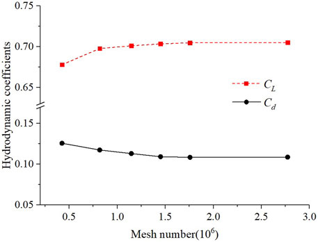
FIGURE 3. Time-averaged lift and draft coefficients against mesh number.

Table 1 summarises the six test grids under the test conditions to verify the grid independence. It includes the average pressure value P₁ on the suction surface at x/C = 0.4, and the average pressure value P₂ on the pressure surface at x/C = 0.32. The table presents that case 5 and case 6 have similar characteristics, and both can meet the grid requirements for LES. We choose case 5 as the final grid to reduce the computational workload, and the number of grids is approximately 1.7 million.

TABLE 1

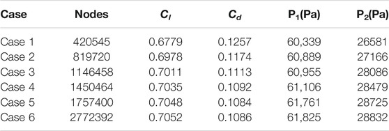
TABLE 1. Verification of grid independence.

Results and Discussions

Verification of Numerical Simulation Methods

Figure 4 shows the numerical simulation results of the transient cavitating flow distribution of the three types of bionic hydrofoils and the Clark-y hydrofoil. The setting of numerical conditions is completely consistent with experimental setting (Huang et al., 2012; Roohi et al., 2013). The figure presents that the cavitation circumfluence in a cycle can be roughly divided into four stages. In the first stage, an attached cavity forms at the leading-edge, and the cavity at the trailing edge begins to fall off. In the second stage, the attached cavity gradually increases and forms a sheet cavity, and the influence range of cavitation is the largest. In the third stage, the sheet cavitation breaks up gradually, separates and falls off, forming cloud cavitation, and the influence range of cavitation becomes small. In the fourth stage, the cavity gradually moves from the leading-edge to the trailing edge. At this time, the cavity of the hydrofoil is mainly concentrated at its trailing edge, and the influence range of cavitation is the smallest. Afterwards, the attached cavity is generated again at the leading-edge, which represents the beginning of the next cycle. Figure 4 depicts that the numerical simulation can accurately observe the transient cavitating flow change process under different hydrofoil schemes. Comparison of the results of the four-stage numerical simulation with experimental results shows a high degree of agreement, which proves the correctness of the numerical calculation method in this paper. The numerical simulation and experimental values of clark-y hydrofoil are given on the right side of Table 2 [numerical simulation is carried out under the same experimental conditions as Wei et al. (2011)]. It can be seen that both the lift coefficient and the drag coefficient are very close to the experimental value, and the maximum error is 1.68%, which is within the allowable error range. Further, according to the formula $Sr=lf/v$, the experimental Strouhal number is 0.169 and the numerical simulation Strouhal number is 0.176. The relative error between them is 3.98%, which can meet the similarity criterion of flow unsteady. This further verifies the accuracy of the numerical simulation in this paper.

FIGURE 4

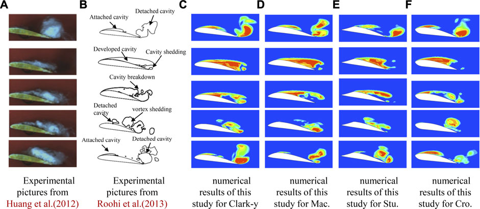
FIGURE 4. Cavitation experimental results and numerical simulation results of different hydrofoils in a single cycle. (A) Experimental pictures from Huang et al. (2012) (B) Experimental pictures from Roohi et al. (2013) (C) Numerical results of this study for Clark-y (D) Numerical results of this study for Mac. (E) Numerical results of this study for Stu. (F) Numerical results of this study for Cro.

TABLE 2

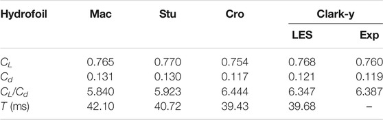
TABLE 2. Average lift–drag coefficient and lift-to-drag ratio and cavitation cycle (T) of each hydrofoil.

Comparison of Lift and Drag Characteristics

Figure 5 shows the transient change curves of the lift coefficient C_L and drag coefficient C_d of the four hydrofoils over a while. The left side of the coordinate axis represents the value of C_L, and the right side represents the value of C_d. C_L and C_d of the four hydrofoils fluctuate periodically over time, and the value of C_L is always greater than the value of C_d. Their fluctuations are also always synchronised, that is, crests and troughs appear at the same time. Depending on the scheme, the period and amplitude of the fluctuations in the values of C_L and C_d differ, which shows that a change in the leading-edge structure will have a certain effect on the lift and drag characteristics of the hydrofoils. The Cro. scheme has the largest amplitude, whereas the Stu. scheme has the smallest amplitude. The average values of C_L and C_d for each scheme in Table 2 indicate that the average lift coefficients of the four hydrofoils are relatively close, but the lift coefficient of the Stu. hydrofoil is relatively larger. For the average drag coefficient, the four hydrofoils have small differences, but the average drag coefficient of the Cro. hydrofoil is the smallest. Table 2 also provides the lift-to-drag ratios of the four hydrofoils to measure their lift–drag characteristics clearly. The lift-to-drag ratio of the Cro. hydrofoil is significantly greater than those of the two other bionic hydrofoils, and it is also slightly higher than that of the traditional Clark-y hydrofoil.

FIGURE 5

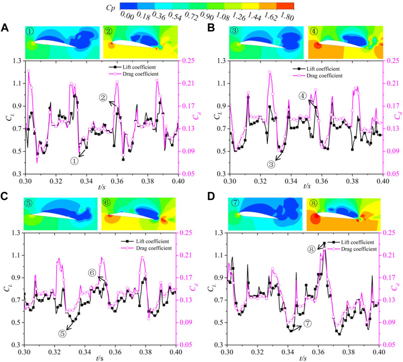
FIGURE 5. Transient lift–drag coefficient curves and pressure coefficient Cp cloud diagrams of the four hydrofoils. (A) Clark-y (B) Mac. (C) Stu. (D) Cro.

The upper part of each curve in Figure 5 shows the pressure coefficient C_p cloud diagram of the four hydrofoils at the peak and trough of the C_L curve. The expression is

$C_p=\frac{p}{0.5\rho U_0^2}(12)$

$p$ represents the pressure value in space coordinates. The figure demonstrates that the C_p value of the pressure surface of the hydrofoils is always higher than that of the suction surface regardless of when the lift coefficient is the largest or smallest, and the value reaches the maximum at the front and trailing edges of the pressure surface. When the lift coefficient changes from the trough to the crest, the low-pressure area on the suction surface of the hydrofoils gradually decreases and moves to the trailing edge. On the contrary, the high-pressure area on the pressure surface of the hydrofoils gradually expands and mainly concentrates on the leading and trailing edges. The pressure difference between the suction and pressure surface is the fundamental reason for the lift of hydrofoils. When the low-pressure area of the hydrofoils is large, the pressure difference of hydrofoil is also great which can obtain a good lift. Comparison of C_p cloud images of the four hydrofoils at the wave crests shows that the pressure surface of the Cro. hydrofoil has the widest high-pressure area, and the lift coefficient is also the largest. From the C_p cloud picture at the trough, the low-pressure area on the suction surface of the Cro. hydrofoil is the widest. On the basis of the lift–drag ratios in Table 2, the Cro. hydrofoil has a better lift–drag characteristics than the others.

Evolution of Transient Cavitating Flow

We use the C_L curve as a basis, regard one wave trough to the next wave trough as a cycle and provide the cavitation evolution diagram of the four hydrofoils in one cycle, as shown in Figure 6. The cavitation process of the four hydrofoils changes periodically with the change in C_L. When C_L is in the trough position, a thin attached cavity is produced at the leading-edge of the hydrofoils, and the cloud cavity generated in the previous cycle at the trailing edge is gradually falling off. At moment ①, the cloud cavitation at the trailing edge falls off and leaves the hydrofoil surface, whilst the attached cavity at the leading-edge gradually extends backward until the cavity covers the suction surface to form sheet cavitation. At time ②, the sheet cavitation continues to move to the trailing edge of the hydrofoils, the cavity begins to break in the middle and rear parts, and the volume of the cavity reaches the maximum at this time. At time ③, the sheet cavitation is breaking down, the cavitation of the leading-edge is gradually reduced, and the cavitation area of the hydrofoils is gradually divided into two parts. When time ④ is reached, the cavitation at the leading-edge disappears, the cavity is mainly concentrated near the trailing edge, and the influence range of cavitation is the smallest. Time ⑤ is another trough. The attached cavity reappears, and the cloud cavitation at the trailing edge begins to fall off. This phenomenon indicates that the evolution of the hydrofoil cavitation begins to enter the next cycle.

FIGURE 6

FIGURE 6. Transient evolution process of the cavitating flow of the four hydrofoils in one cycle. (10% vapor volume fraction iso-surface) (A) Clark-y (B) Mac. (C) Stu. (D) Cro.

The figure illustrates that the cavitation evolution of the four hydrofoils is similar, but some differences exist. The cavitation of the Stu. hydrofoil is slightly different from that of the three other types of hydrofoils. The Stu. hydrofoil always has a thin attached cavity at the leading-edge, and the subsequent series of cavitation evolution occurs close to the maximum thickness of the hydrofoil (approximately x/C = 0.25). The cavitation evolution of the other three hydrofoils starts from the leading-edge. The Cro. hydrofoil cavitation occurs more forward than the others, whereas the Mac. hydrofoil cavitation occurs more rearward. At time ②, the sheet cavitation of the Cro. hydrofoil has been basically broken, whilst the remaining three hydrofoils have just started to break. This condition may be due to the upturning of the leading-edge, resulting in the early break of its sheet cavitation. The last line of Table 2 shows the average cavitation cycle of the four hydrofoils. It can be seen from the table that the cavitation cycle of the Cro. hydrofoil (T = 39.43 ms) is the shortest and that of the Mac. Hydrofoil (T = 42.10 ms) is the longest. This further shows that the change of hydrofoil leading-edge will affect the evolution of cavitation. When the characteristic curve of the hydrofoil leading-edge is Cro. model, the hydrofoil can have a shorter cavitation evolution cycle.

Figure 7 shows the curves of the density distribution (averaged in one cycle) on the suction surface of the four hydrofoils to consider the cavitation evolution of the hydrofoils. The position of the Cro. hydrofoil cavitation occurs earlier (approximately x/C = 0.03) than that of the others, whereas the position of the Mac. hydrofoil cavitation occurs later (approximately x/C = 0.124). For the Stu. hydrofoil, cavitation has already appeared at the forefront of the hydrofoil, and the cavitation range ends at x/C = 0.099. The subsequent evolution of cavitation starts at x/C = 0.241. This is consistent with the results observed in the 3D cavitation evolution of the hydrofoil in Figure 6. The cavitation of the hydrofoils is mainly concentrated in their middle section, and it is the most serious at approximately x/C = 0.21–0.23. As the cavity stretches along the hydrofoils, the density fields of the hydrofoils rise. After the trailing edge is approached, the density fields of the four hydrofoils drop again slightly.

FIGURE 7

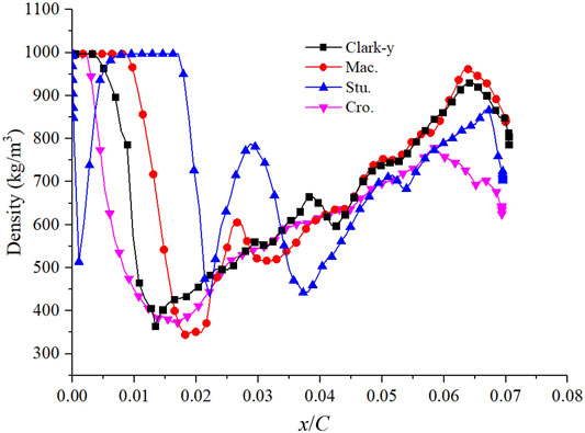
FIGURE 7. Average density distribution on the suction surface of the four hydrofoils, $\sigma =0.8$.

The occurrence of cavitation will inevitably lead to changes in the cavity velocity. Figure 8 shows the time-averaged x-velocity distribution of the four types of hydrofoils. The upper part of Figure 8 shows the location of the selected area (taking Clark-y hydrofoil as an example, the other hydrofoils are the same). The figure indicates that the velocity fluctuation is related to the selected position of the hydrofoil sections. From the Y-axis direction, the velocity near the walls of the hydrofoils shows great fluctuations; the higher the upward tilt is, the more the velocity fluctuations tend to be stable. As the fluid particle moves towards the trailing edge of the hydrofoils, the influence range of the velocity fluctuation in the Y-axis direction gradually increases. Especially at x/C = 1.2, velocity fluctuations exist in the Y-axis direction, indicating that the cavity will continue to move backward after falling off the surface of the hydrofoils. The size of the velocity fluctuation is related to the thickness of the cavity, and the velocity fluctuation of the Cro. hydrofoil is the smallest. The figure also shows the experimental results of Li et al. (2017). The velocity fluctuations of the four hydrofoils tend to be in good agreement with the experimental results.

FIGURE 8

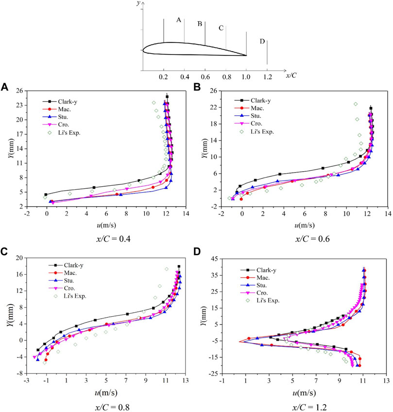
FIGURE 8. Time-averaged velocity fluctuation curve along the flow direction around the four hydrofoils.

Vortex Evolution

The transient cavitating flow of the hydrofoils is closely related to the vortex structure. We use the $Q$ criterion to study the structure of the vortex, which is an important method to study the vortex in transient cavitation flow (Yu et al., 2020). It is defined as follows:

$Q=\frac{\left({\mathrm{\Omega }}^2-S^2\right)}{2}(13)$

Amongst them, $Q$ is the second invariant of the velocity gradient tensor, $\Omega$ represents the vorticity amplitude, and $S$ represents the strain rate tensor. The magnitude of its value can be used to identify the relationship between vorticity and strain rate. When $Q>0$, the rotation effect is dominant; when $Q<0$, the shearing effect is dominant.

Figure 9 shows $Q$ distribution of the four hydrofoils. It can be seen from the figure that the $Q$ distribution of Clark-y hydrofoil is significantly different from that of the three bionic hydrofoils. In the whole cycle, the negative $Q$ area of Clark-y hydrofoil is always larger than that of the other three bionic hydrofoils, which shows that the shear effect of Clark-y hydrofoil is dominant when cavitation shedding. The vortex evolution of the three bionic hydrofoils is similar. Take Mac. hydrofoil as an example, in the initial stage (1/5T), $Q$ of the leading-edge is mainly negative, and $Q$ towards the trailing edge becomes positive. The rotation effect of the hydrofoil at the trailing edge is dominant at this time. When the sheet cavitation begins to break (2/5T), the negative $Q$ area near the trailing edge begins to increase gradually, and the shear effect begins to become evident. When the break of the hydrofoil cavity intensifies (3/5T), the negative $Q$ area appears widely. At this time, the positive $Q$ and negative $Q$ areas alternately appear, and the rotation and shear effects jointly dominate the cavitation flow. When the cavity moves further back (4/5T), cavitation is mainly concentrated at the trailing edge. $Q$ value is mainly positive at this time given no shedding of the cavity, and the rotation effect is dominant. With continuous development, an attached cavity is formed at the leading-edge, and the cavitation at the trailing edge begins to fall off the hydrofoil surface (5/5T). At this time, the cavitating flow becomes unstable, and rotation- and shear-dominant areas appear on the cavity surface.

FIGURE 9

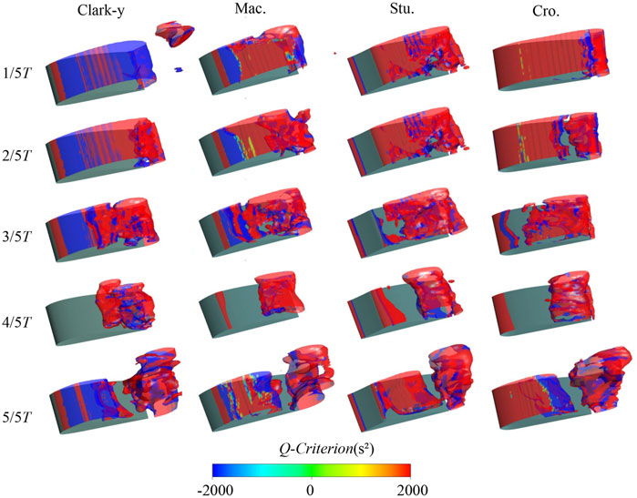
FIGURE 9. Comparison of the vortex structures around the four hydrofoils based on $Q$ criterion.

However, there are still differences among the three bionic hydrofoils. In the initial stage, the negative $Q$ area of the front edge of the Mac. hydrofoil is more obvious; when the sheet cavitation breaks, the shear effect of the Mac. hydrofoil is more significant. The positive $Q$ area of the leading-edge of the Cro. hydrofoil is significantly wider, indicating that the rotation effect of the Cro. hydrofoil is more obvious. This result shows that in unsteady cavitating flow, rotation and shear jointly control the cavitation evolution. When the leading-edge structure is changed, the evolution of the hydrofoil vortex will also be affected.

The vorticity transport equation is used to compare and analyse the vorticity on the three bionic hydrofoils to study the cavitation–vortex interaction. The equation is as follows:

$\frac{D\overrightarrow{\omega }}{Dt}=\left(\overrightarrow{\omega }\cdot \nabla \right)\overrightarrow{V}-\overrightarrow{\omega }\left(\nabla \cdot \overrightarrow{V}\right)+\frac{\nabla {\rho }_m\times \nabla p}{\nabla {\rho }_m^2}+\left({\nu }_m+{\nu }_t\right){\nabla }^2\overrightarrow{\omega }(14)$

The vortex-stretching term $\left(\overrightarrow{\omega }\cdot \nabla \right)\overrightarrow{V}$ reveals the stretching and tilting of the vortex caused by the velocity gradient. The vortex dilatation term $\overrightarrow{\omega }\left(\nabla \cdot \overrightarrow{V}\right)$ is affected by volume expansion or contraction. $\frac{\nabla {\rho }_m\times \nabla p}{\nabla {\rho }_m^2}$ is the vortex baroclinic term, which describes the effect of the baroclinic moment on the vorticity due to the nonparallel pressure gradient and density gradient. $\left({\nu }_m+{\nu }_t\right){\nabla }^2\overrightarrow{\omega }$ of different bionic hydrofoils slightly changes, but this change is minimal and is thus usually ignored.

Figure 10 shows the distribution of total vorticity and the three directional vorticities of the four hydrofoils on the cavity surface at the same time (t = 0.4 s). Vorticity distribution in the Z direction is similar to the total vorticity, and the vorticity in the Z direction is much larger than the vorticity distribution in the other two directions. Therefore, the vorticity dynamics of the three bionic hydrofoils are evaluated by analyzing the vorticity Z.

FIGURE 10

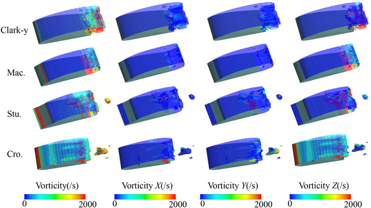
FIGURE 10. Distribution of total vorticity, vorticity X, vorticity Y and vorticity Z of the four hydrofoils at the same time (t = 60 ms).

The vortex-stretching term is related to the velocity gradient, and cavitation will have a significant effect on the velocity gradient in the transient flow. As shown in Figure 11, in the initial stage (1/5T), only a small range of vortex stretching is evident. Cavitation is in the developing stage, and the velocity gradient does not change much. With the development of cavitation (2/5T), a re-entrant flow gradually forms and develops, causing the velocity gradient of the hydrofoil surface to change. At this time, the influence range of the vortex-stretching term gradually increases. When the sheet cavitation gradually breaks (3/5T), the scope of influence of this item further increases and gradually extends to the entire surface of the hydrofoils. When the sheet cavitation is completely broken, the cavitation begins to move to the trailing edge of the hydrofoils, and the leading-edge cavitation begins gradually (4/5T–5/5T). At this time, the growth of the cavity slows down, the velocity gradient change is small, and the influence range of the vortex-stretching term gradually decreases.

FIGURE 11

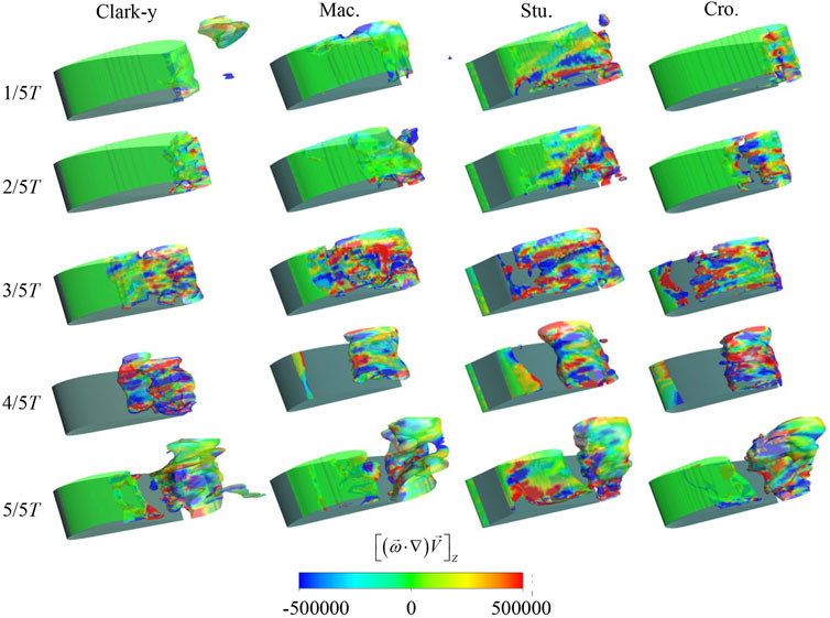
FIGURE 11. Comparison of the Z-direction vortex-stretching term evolution of the four hydrofoils in a typical cycle.

The change trends of the vortex-stretching term of the four hydrofoils are generally similar. However, there are still differences. Compared with the bionic hydrofoil, the variation area of the vortex-stretching term of Clark-y hydrofoil in the initial stage of cavitation is smaller, but when the cavity begins to shedding from the living cavity, the vortex stretching term begins to change dramatically. The stretching term of vortices of the three bionic hydrofoils changes gently in the whole cycle, and the change of the velocity gradient of the Stu. hydrofoil in each stage is more obvious, especially near the leading-edge. This is because the flat structure of the leading-edge is more conducive to the formation and development of re-entrant flow, resulting in greater changes in velocity gradient. When the attached cavitation of Cro. hydrofoil is formed, the area with zero vortex-stretching term accounts for a larger proportion, and the change of velocity gradient is the smallest.

The vortex dilatation term mainly refers to the change in fluid volume that affects the vortex. Due to cavitation, the volume of the fluid will change, causing the vorticity to also change. Figure 12 shows the distribution of the vortex dilatation term of the four hydrofoils in a typical period. In the 1/5T stage, the vortex expansion is concentrated near the trailing edge, and the vortex dilatation term of the leading-edge is small. When the cavitation develops to the 2/5T stage, an attached cavity gradually develops, and the volume change rate gradually increases. When the sheet cavitation begins to break (3/5T), the volume changes drastically, and the value of the vortex dilatation term reaches the maximum at the break of the cavity. When the sheet cavitation is completely broken to form cloud cavitation (4/5T), the positive and negative values of the vortex dilatation term appear alternately. Afterwards, the value of the vortex dilatation term gradually decreases due to the slow formation of the attached cavity (5/5T).

FIGURE 12

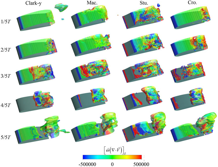
FIGURE 12. Comparison of the Z-direction vortex dilatation term evolution of the four hydrofoils in a typical cycle.

In the initial stage of the cavitation evolution cycle, the fluid volume change rate of Clark-y hydrofoil and Mac. hydrofoil is low, and the dilatation term of the vortex is mainly zero. However, at 3/5T, due to the shedding of sheet cavitation, the fluid volume changes sharply, resulting in a sharp decrease in the zero value region of the dilatation term. The zero value area of the vortex dilatation term of the Stu. hydrofoil in the whole cavitation evolution cycle is low, indicating that its fluid volume changes most dramatically. The warping of hydrofoil leading-edge structure will affect the change of vortex dilatation rate.

The vortex baroclinic term is related to the variation of nonparallel pressure and density. For a general positive pressure fluid, pressure and density have the same gradient, that is, zero. For an unsteady cavitating flow, these two items are not always the same, which will cause the change of the vorticity. Figure 13 shows the distribution of vortex baroclinic terms for the four hydrofoils. The vortex baroclinic terms mainly exist in the leading-edge of the hydrofoils and the area where the sheet cavitation is broken. The occurrence of the attached cavity or the break of the cavity will cause a gas-liquid two-phase transition, which in turn will change the density gradient of the flow field. Although the influence range of this term is smaller than those of the above two terms, it plays an important role in the generation of vortices. The baroclinic term of the Mac. hydrofoil and Clark-y hydrofoil are more complex when cavitation breaks (3/5T). When attached cavitation occurs (5/5T), the baroclinic term of the Cro. hydrofoil is more stable. The change in the vortex of the flow field will also change due to the influence of cavitation, and the change in the leading-edge structure will affect the evolution of the hydrofoil vortex.

FIGURE 13

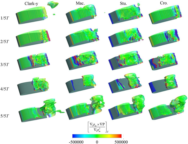
FIGURE 13. Comparison of the Z-direction vortex baroclinic term evolution of the four hydrofoils in a typical cycle.

Conclusion

This study uses geometrical bionic principles to establish three bionic hydrofoils with evident leading-edge structural differences and calculates the lift and drag coefficients, transient cavitating flow and vortex evolution of the hydrofoils by using the LES method. On the basis of comparison and analysis, the conclusions are as follows:

1) From the comparison of the numerical simulation and experimental results of the transient cavitating flow of four hydrofoils in a period, their cavitation evolution process is always similar. Regardless of the location where the attached cavity occurs, the size of the sheet cavitation and the location of its break and the shape of the cloud cavitation, the numerical simulation and experimental results show a high degree of agreement. This agreement verifies the accuracy of the numerical simulation method in this paper.

2) The lift and drag coefficients of the three bionic hydrofoils and the Clark-y hydrofoil are inconsiderably different in general, but the lift–drag ratio of the Cro. hydrofoil is better. Comparison of C_p cloud images of the four hydrofoils shows that when C_L reaches the peak, the pressure surface of the Cro. hydrofoil has the widest high-pressure area. When C_L is in the trough, the low-pressure area of the Cro. hydrofoil is the widest. The Cro. hydrofoil has better lift and drag characteristics than the others.

3) The position of the attached cavity of a hydrofoil will change due to the change in the leading-edge structure. When the leading-edge structure is upturned, the position of the attached cavity will move forward. The position where the attached cavity of the Stu. hydrofoil occurs is the rearmost (approximately x = 16.9 mm). The position where the attached cavity of the Cro. Hydrofoil occurs is the most forward (approximately x = 2.9 mm), and the velocity fluctuation at its trailing edge is the smallest. From the perspective of the cavitation evolution period, the cavitation evolution period of the Cro. hydrofoil is shorter (approximately T = 27 ms) than that of the others, whereas the cavitation period of the Mac. hydrofoil is longer (approximately T = 31 ms).

4) The warping of leading-edge structure will cause significant changes in the vortex evolution of hydrofoils. The Mac. hydrofoil has a wider negative $Q$ area at the leading-edge compared with others, whereas the rotation effect of the Cro. hydrofoil is more obvious than that of the others. When the leading-edge structure is tilted downward, the changes in the vortex stretching and dilatation terms of the hydrofoils, particularly the Stu. hydrofoil, are complicated, and their vortex has a wide range of influence.

Data Availability Statement

The original contributions presented in the study are included in the article/Supplementary Material, further inquiries can be directed to the corresponding author.

Author Contributions

All authors contributed to this research. HZ conducted the experiments, performed the experiments, and wrote the draft of this paper. HY, JW, TS, and FQ suggested the study idea and shared in writing and revising the paper.

Funding

This work was supported by the University Synergy Innovation Program of Anhui Province under Grant No. GXXT-2019-004, the Fundamental Research Funds for the Central Universities (NO: JZ2021HGTB0090), the financial support provided by the National Natural Science Foundation of China (51806053) and Anhui Provincial Key Research and Development Program (Grant No. 201904a05020070, 1804a09020012 and 1804a09020007).

Conflict of Interest

Author JW is employed by Hefei Kaiquan Electric Motor Pump Co., Ltd. Author TS is employed by Hefei Hengda Jianghai Pump Co., Ltd.

The remaining authors declare that the research was conducted in the absence of any commercial or financial relationships that could be construed as a potential conflict of interest.

Publisher’s Note

All claims expressed in this article are solely those of the authors and do not necessarily represent those of their affiliated organizations, or those of the publisher, the editors and the reviewers. Any product that may be evaluated in this article, or claim that may be made by its manufacturer, is not guaranteed or endorsed by the publisher.

References

Amini, A., Reclari, M., Sano, T., Iino, M., and Farhat, M. (2019). Suppressing Tip Vortex Cavitation by Winglets. Exp. Fluids 60, 159. doi:10.1007/s00348-019-2809-z

CrossRef Full Text | Google Scholar

Antoine, D., Jacques, A. A., François, D., and Sigrist, J. F. (2009). Fluid Structure Interaction Analysis on a Transient Pitching Hydrofoil. Am. Soc. Mech. Eng. 4, 665–671. doi:10.1115/pvp2009-78082

CrossRef Full Text | Google Scholar

Arabnejad, M. H., Amini, A., Farhat, M., and Bensow, R. E. (2019). Numerical and Experimental Investigation of Shedding Mechanisms from Leading-Edge Cavitation. Int. J. Multiphase Flow 119, 123–143. doi:10.1016/j.ijmultiphaseflow.2019.06.010

CrossRef Full Text | Google Scholar

Cheng, H., Long, X., Ji, B., Peng, X., and Farhat, M. (2019). LES Investigation of the Influence of Cavitation on Flow Patterns in a Confined Tip-Leakage Flow. Ocean Eng. 186, 106115. doi:10.1016/j.oceaneng.2019.106115

CrossRef Full Text | Google Scholar

Custodio, D., Henoch, C., and Johari, H. (2018). Cavitation on Hydrofoils with Leading Edge Protuberances. Ocean Eng. 162, 196–208. doi:10.1016/j.oceaneng.2018.05.033

CrossRef Full Text | Google Scholar

Fujii, A., Kawakami, D. T., Tsujimoto, Y., and Arndt, R. E. (2007). Effect of Hydrofoil Shapes on Partial and Transitional Cavity Oscillations. J. Fluids Eng. 129, 669–673. doi:10.1115/1.2734183

CrossRef Full Text | Google Scholar

Garg, N., Pearce, B. W., Brandner, P. A., Phillips, A. W., Martins, J. R. R. A., and Young, Y. L. (2019). Experimental Investigation of a Hydrofoil Designed via Hydrostructural Optimization. J. Fluids Structures 84, 243–262. doi:10.1016/j.jfluidstructs.2018.10.010

CrossRef Full Text | Google Scholar

Hicks, R. M., and Henne, P. A. (1978). Wing Design by Numerical Optimization. J. Aircraft 15, 407–412. doi:10.2514/3.58379

CrossRef Full Text | Google Scholar

Hong, J., Qian, Z. H., and Ren, L. Q. (2009). Extensive Model of Multi-Factor Coupling Bionics and Analysis of Coupling Elements. J. Jilin University(Engineering Tech. Edition) 39, 726–731. doi:10.1061/41039(345)45

CrossRef Full Text | Google Scholar

Hu, C., Chen, G., Yang, L., and Wang, G. (2018). Large Eddy Simulation of Turbulent Attached Cavitating Flows Around Different Twisted Hydrofoils. Energies 11, 2768. doi:10.3390/en11102768

CrossRef Full Text | Google Scholar

Huang, B., Wang, G., Yu, Z., and Shi, S. (2012). Detached-eddy Simulation for Time-dependent Turbulent Cavitating Flows. Chin. J. Mech. Eng. 25, 484–490. doi:10.3901/cjme.2012.03.484

CrossRef Full Text | Google Scholar

Huang, B., Wang, G. Y., and Yuan, H. T. (2010). A Cavitation Model for Cavtating Flow Simulations. J. Hydrodynamics, Ser.B. 22, 798–804. doi:10.1016/s1001-6058(10)60033-9

CrossRef Full Text | Google Scholar

Huang, R., Luo, X., and Ji, B. (2017). Numerical Simulation of the Transient Cavitating Turbulent Flows Around the Clark-Y Hydrofoil Using Modified Partially Averaged Navier-Stokes Method. J. Mech. Sci. Technol. 31, 2849–2859. doi:10.1007/s12206-017-0528-z

CrossRef Full Text | Google Scholar

Huang, S. X., Hu, Y., and Wang, Y. (2020). Research on Aerodynamic Performance of a New Dolphin Head-Based Bionic Airfoil. Energy 11, 118179. doi:10.1016/j.energy.2020.118179

CrossRef Full Text | Google Scholar

Ji, B., Long, Y., Long, X.-p., Qian, Z.-D., and Zhou, J.-j. (2017). Large Eddy Simulation of Turbulent Attached Cavitating Flow with Special Emphasis on Large Scale Structures of the Hydrofoil Wake and Turbulence-Cavitation Interactions. J. Hydrodyn 29, 27–39. doi:10.1016/s1001-6058(16)60715-1

CrossRef Full Text | Google Scholar

Ji, B., Luo, X. W., Arndt, R. E. A., Peng, X., and Wu, Y. (2015). Large Eddy Simulation and Theoretical Investigations of the Transient Cavitating Vortical Flow Structure Around a NACA66 Hydrofoil. Int. J. Multiphase Flow 68, 121–134. doi:10.1016/j.ijmultiphaseflow.2014.10.008

CrossRef Full Text | Google Scholar

Kim, J., and Lee, J. S. (2015). Numerical Study of Cloud Cavitation Effects on Hydrophobic Hydrofoils. Int. J. Heat Mass Transfer 83, 591–603. doi:10.1016/j.ijheatmasstransfer.2014.12.051

CrossRef Full Text | Google Scholar

Kulfan, B. M. (2008). Universal Parametric Geometry Representation Method. J. Aircraft 45, 142–158. doi:10.2514/1.29958

CrossRef Full Text | Google Scholar

Li, L., Li, B., Hu, Z., Lin, Y., and Cheung, S. C. P. (2016). Large Eddy Simulation of Unsteady Shedding Behavior in Cavitating Flows with Time-Average Validation. Ocean Eng. 125, 1–11. doi:10.1016/j.oceaneng.2016.07.065

CrossRef Full Text | Google Scholar

Li, Z., Zheng, D., Hong, F., and Ni, D. (2017). Numerical Simulation of the Sheet/cloud Cavitation Around a Two-Dimensional Hydrofoil Using a Modified URANS Approach. J. Mech. Sci. Technol. 31, 215–224. doi:10.1007/s12206-016-1224-0

CrossRef Full Text | Google Scholar

Liu, X., and Liu, X. (2014). A Numerical Study of Aerodynamic Performance and Noise of a Bionic Airfoil Based on Owl wing. Adv. Mech. Eng. 6, 859308. doi:10.1155/2014/859308

CrossRef Full Text | Google Scholar

Liu, Y., and Tan, L. (2020). Method of T Shape Tip on Energy Improvement of a Hydrofoil with Tip Clearance in Tidal Energy. Renew. Energ. 149, 42–54. doi:10.1016/j.renene.2019.12.017

CrossRef Full Text | Google Scholar

Marimon Giovannetti, L., Banks, J., Ledri, M., Turnock, S. R., and Boyd, S. W. (2018). Toward the Development of a Hydrofoil Tailored to Passively Reduce its Lift Response to Fluid Load. Ocean Eng. 167, 1–10. doi:10.1016/j.oceaneng.2018.08.018

CrossRef Full Text | Google Scholar

Masters, D. A., Poole, D. J., Taylor, N. J., Rendall, T. C. S., and Allen, C. B. (2017). Influence of Shape Parameterization on a Benchmark Aerodynamic Optimization Problem. J. Aircraft 54, 1–15. doi:10.2514/1.c034006

CrossRef Full Text | Google Scholar

Oller, S., Nallim, L., and Oller, S. (2016). Usability of the Selig S1223 Profile Airfoil as a High Lift Hydrofoil for Hydrokinetic Application. J. Appl. Fluid Mech. 9, 537–542. doi:10.18869/acadpub.jafm.68.225.24302

CrossRef Full Text | Google Scholar

Rajaram, A. N., and Srikanth, N. (2020). Multi-objective Optimization of Hydrofoil Geometry Used in Horizontal axis Tidal Turbine Blade Designed for Operation in Tropical Conditions of South East Asia. Renew. Energ. 146, 166–180. doi:10.1016/j.renene.2019.05.111

CrossRef Full Text | Google Scholar

Roohi, E., Zahiri, A. P., and Passandideh-Fard, M. (2013). Numerical Simulation of Cavitation Around a Two-Dimensional Hydrofoil Using VOF Method and LES Turbulence Model. Appl. Math. Model. 37, 6469–6488. doi:10.1016/j.apm.2012.09.002

CrossRef Full Text | Google Scholar

Sun, T., Wang, Z., Zou, L., and Wang, H. (2020). Numerical Investigation of Positive Effects of Ventilated Cavitation Around a NACA66 Hydrofoil. Ocean Eng. 197, 106831. doi:10.1016/j.oceaneng.2019.106831

CrossRef Full Text | Google Scholar

Wang, S., Zhu, J., Xie, H., Zhang, F., and Zhang, X. (2019). Studies on thermal Effects of Cavitation in LN2 Flow over a Twisted Hydrofoil Based on Large Eddy Simulation. Cryogenics 97, 40–49. doi:10.1016/j.cryogenics.2018.11.007

CrossRef Full Text | Google Scholar

Wei, Y.-J., Tseng, C.-C., and Wang, G.-Y. (2011). Turbulence and Cavitation Models for Time-dependent Turbulent Cavitating Flows. Acta Mech. Sin. 27, 473–487. doi:10.1007/s10409-011-0475-3

CrossRef Full Text | Google Scholar

Xue, G., Liu, Y., Zhang, M., Zhang, W., Zhang, J., Luo, H., et al. (2016). Optimal Design and Numerical Simulation on Fish-like Flexible Hydrofoil Propeller. Polish Maritime Res. 23, 59–66. doi:10.1515/pomr-2016-0070

CrossRef Full Text | Google Scholar

You, C., Zhao, G., Chu, X., Zhou, W., Long, Y., and Lian, Y. (2020). Design, Preparation and Cutting Performance of Bionic Cutting Tools Based on Head Microstructures of Dung Beetle. J. Manufacturing Process. 58, 129–135. doi:10.1016/j.jmapro.2020.07.057

CrossRef Full Text | Google Scholar

Yu, A., Qian, Z. H., Wang, X. C., Tang, Q. H., and Zhou, D. Q. (2020). Large Eddy Simulation of Ventilated Cavitation with an Insight on the Correlation Mechanism between Ventilation and Vortex Evolutions. Appl. Math. Model. 89, 1055–1073. doi:10.1016/j.apm.2020.08.011

CrossRef Full Text | Google Scholar

Zhang, D.-s., Shi, W.-d., Zhang, G.-j., Chen, J., and van Esch, B. P. M. B. (2017). Numerical Analysis of Cavitation Shedding Flow Around a Three-Dimensional Hydrofoil Using an Improved Filter-Based Model. J. Hydrodyn 29, 361–375. doi:10.1016/s1001-6058(16)60746-1

CrossRef Full Text | Google Scholar

Zhang, D., Shi, W., Pan, D., and Zhang, G. (2015). Numerical Simulation of Cavitation Shedding Flow Around a Hydrofoil Using Partially-Averaged Navier-Stokes Model. Int. J. Numer. Methods Heat Fluid Flow 25, 825–830. doi:10.1108/hff-05-2014-0150

CrossRef Full Text | Google Scholar

Zhang, M. J., Huang, B., Qian, Z. D., Liu, T. T., Wu, Q., Zhang, H. Z., et al. (2020). Cavitating Flow Structures and Corresponding Hydrodynamics of a Transient Pitching Hydrofoil in Different Cavitation Regimes. Int. J. Multiphase Flow 132, 103408. doi:10.1016/j.ijmultiphaseflow.2020.103408

CrossRef Full Text | Google Scholar

Zhou, L. J., Guo, Q., and Wang, Z. W. (2016). Numerical Evaluation of the Clearance Geometries Effect on the Flow Field and Performance of a Hydrofoil. Renew. Energ. 99, 390–397. doi:10.1016/j.renene.2016.06.064

CrossRef Full Text | Google Scholar

201904a05020070 1804a09020012