 Bo Chen
 Xiaojun Li
 Zuchao Zhu
94% of researchers rate our articles as excellent or good
Learn more about the work of our research integrity team to safeguard the quality of each article we publish.
Find out more
ORIGINAL RESEARCH article
Front. Energy Res., 31 January 2022
Sec. Process and Energy Systems Engineering
Volume 9 - 2021 | https://doi.org/10.3389/fenrg.2021.818232
This article is part of the Research TopicDesign, Simulation and Optimization of Hydraulic MachineryView all 25 articles
Time-resolved particle image velocimetry (TR-PIV) measurements were conducted to analyze the unsteady flow field developing in a centrifugal pump. The flow structures in the impeller passage under different flow rates were investigated. The overall statistical characteristics of the flow were obtained with the study of relative phase-averaged flow field, phase-averaged turbulent kinetic energy (TKE), and the analysis of frequency. Through the study of the first few proper orthogonal decomposition (POD) modes of the flow field, the coherent flow structures under several flow rates were revealed, consequently, the flow fields were reconstructed by the POD modes. Results show that the main flow structures could be reflected by the first few modes of the flow field: when the fluid follows the blade contour well, the first few modes corresponded to the “jet-wake” structures; when the large-scale flow structures appear in the passage, the 1st and 2nd modes were associated in pairs and corresponded to the stall cells, the 3rd and 4th modes corresponded to the “jet-wake” structures, and the 5th and 6th modes corresponded to the passage vortexes or the “jet-wake” structures (for the extreme part-load conditions). The flow structures that were reflected by the first few modes change as the decrease of flow rate, especially, at the extreme part-load condition, not only the shapes of the flow structures changed, but also the flow direction is reversed. This indicates that the generation mechanism of turbulent kinetic energy in the flow passage changed at the extreme part-load conditions.
Centrifugal pumps consume about 20% of the total generated energy in the world due to their extensive usage in petrochemical, chemical, coal, chemical, pharmaceutical, and other process fields (Arun Shankar et al., 2016; Bozorgasareh et al., 2021). Improving the efficiency and stability of centrifugal pumps is an urgent request for sustainable development (Krause et al., 2005; Keller et al., 2014; Zhang et al., 2020; Zhang et al., 2021). While unsteady flow structures is the core technical problem to centrifugal pumps’ improvement.
Numerous studies have revealed the relationship between the pump operation instability and the unsteady flow structures. Tan et al. (2017) investigated the role of blade rotational angle in the energy performance and pressure fluctuation of a mixed flow pump and found that the maximum amplitude of pressure fluctuation in the impeller at a blade rotational angle of 4° is greater than that of a blade rotational angle at 0°and 4°, the performance was caused by the strong vortex intensity. Santolaria Morros et al. (2011) explored operation characteristics of a pump in reverse mode involved in unsteady flow pattern and forces. These results demonstrated that fluctuations derived from blade-tongue interactions possess up to 25% of steady component, constituting a serious risk of fatigue failure. Xia et al. (2014) investigated the rotating stall of a pump-turbine in pump mode, and they concluded that under rotating stall condition, the enforced rotating non-uniform pressure distribution on the circumference acting on the impellers can result in a stronger sub-synchronous fluctuation of radial force, which leads to rotor-dynamic instabilities and strong vibrations. Moreover, the difference of pressure fluctuations on both sides of the guide vanes induces torque variations, which may have adverse influence on the machine operation. Kaupert (1999) and Kaupert and Staubli (1999) investigated the unsteady pressure field within a high specific speed centrifugal pump impeller, and they found that the hysteresis loop of the pump may be caused by the backflow at the runner outlet and recirculation at the runner inlet.
The analysis of energy loss within a pump reveals that turbulent dissipation could cause the energy loss. Ghorani et al. (2020) studied the irreversible energy losses within the pump as turbine (PAT), and they found that the blade inlet shock, flow deviation at the blade outlet, flow separation, backflow, and vortices in flow passages were categorized as the main reasons for irreversible hydraulic losses within the PAT components. Their results indicate that the turbulent entropy generation is the dominant mechanism for hydraulic losses. Shi et al. (2020) investigated the velocity distribution in the tip clearance of a multiphase pump, their results show that the flow separation phenomenon occurred at the radial coefficient of 0.97 and led to the increase of the turbulent energy loss of the pump. Li et al. (2018a) analyzed the hydraulic loss and flow field in a PAT, their results show that the increase in hydraulic loss in the runner is caused by the backflow and accompanying vortices at the runner inlet near the shroud. On the other hand, the increase in hydraulic loss in the stay/guide vanes is caused by the flow separation and separation vortices near the hub or the shroud. In order to further enrich the theory of rotational stall, Li et al. (2020a) and Li et al. (2020b) explored the mechanism of internal energy loss in the mixed-flow pump under stall conditions. They found that the high-value region of turbulent kinetic energy was basically corresponding to the backflow region of the impeller outlet and the separation region of the boundary layer near the suction surface, which led to a great increase of energy loss in the impeller.
The aforementioned investigations reveal that unsteady flow structures are responsible for the operation stability and energy loss. The flow structures inside the turbomachines are very complicated, including stall sell, flow deviation, flow separation, backflow, and vortices in flow passages, etc. These flow structures overlap and interact with each other, and it is difficult to obtain the characteristics of a single flow structure and the losses. However, when designing the pump, structural optimization is mainly to suppress the main flow structure that produces instability and loss. Therefore, it is necessary to extract these main flow structures from the flow field and analyze their characteristics. Nowadays, the POD method has been widely used to identify the most important and energetic structures dominated in the flow field. Li et al. (2018b) analyzed the airflow characteristics of thermal plumes inside a small space with POD, and the spatial and temporal characteristics of thermal plumes were identified. Lim et al. (2019) extracted POD modes of flow field about the free jets issued from V-notched nozzles, and the results showed that there was energy redistribution from low-order modes to higher-order modes along both PP- and TT-planes of both notched nozzles. Zhou et al. (2021) implemented the POD analysis to reveal the dominant modes of the flow field near the trailing edge of a pitching NACA 0012 airfoil. Tang et al. (2020) used a POD method to decompose the flow structures downstream of a dynamic cylindrical element in a turbulent boundary layer. Yang et al. (2019) applied the POD method to uncover the relation of the instantaneous energetic large-scale turbulent structures to the dominant POD modes. Moreover, POD has also been used to analyze the coherent structures in turbomachines. Han and Tan (2020) used a POD method to decompose the tip leakage vortex in a mixed flow pump as turbine at pump mode and found that POD could capture the main coherent structures of tip leakage vortex. Semlitsch and Mihăescu (2016) applied POD on the analysis of the flow structures appearing in a centrifugal turbocharger compressor. However, the focus of all recent studies has been made on the volute or diffuser, and little research has been done on the flow field characteristics inside the impeller.
In the present work, a TR-PIV system was utilized to measure the flow fields in a special voluteless centrifugal pump. The phase-averaged relative velocities, TKE, and frequency analysis were obtained to analyze the overall statistical characteristics of the flow. The POD method was used to decompose and reconstruct the passage flow. The contributions to the overall energy and the spatial/temporal behavior of the large-scale flow structures were analyzed in detail, and the dynamic and kinematic energy characteristics of the coherent flow structures that were in the impeller were revealed. Understanding the dynamic and energy dissipation characteristics of the unstable flow structure in the pump would allow inventing improved design methods for delaying or suppressing the unstable flow structures.
The pump was subjected to a closed loop (containing a variable frequency drive system, two pressure sensors, three discharge valves, and an electronic flowmeter), which have been already described by Li et al. (2020c). The test pump is a special voluteless centrifugal pump. The impeller and pump casing are made of transparent plexiglass to visualize the flow. Figure 1 shows the test rig and test pump. The main characteristics of the impeller are listed in Table 1. Water was used as working fluid in the pump.
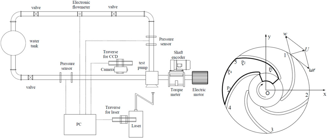
FIGURE 1. Test impeller.
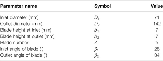
TABLE 1. Impeller geometry.
A TR-PIV system from Lavision was used to obtain a 2D velocity field. The main components are a laser, a laser guiding arm, a high-speed CMOS camera (Phantom Miro 320), and a synchronizer. A commercial software package (DaVis 10.1.2, LaVision) was used to control the image acquisition timing and obtain the velocity fields. The flow was seeded with glass hollow spheres, the diameters ranged from 9–13 μm, and the density is 1050 kg/m3. During the test, the particles were scattered well in the pump. The laser guiding arm and light sheet optics system forms a light sheet of 1 mm thickness and directed along the mid-plane of the impeller. The CMOS camera with 1920 × 1200 pixels was used to acquire images, a Nikkor f = 50 mm, f/1.4 objective from Nikon Corporation was used and an optical filter with a 527-nm high pass filter was installed in front of the camera in order to increase signal-to-noise ratios. The camera was aligned perpendicularly to the laser sheet. The acquisition area contains a complete flow path with a resolution of 0.13 mm/pixel. The maximum frame rate of the camera is 1380 Hz at full resolution, and the minimum frame interval is 1.4 μs. A triggering system (shaft encoder) was used on the rotating shaft, and images were acquired in the same phase of each cycle. The images were processed by the LaVision Davis 10.1.2 software. The multiple interrogation method was used to process the images. The interrogation windows decrease in size in successive iterations: 64 × 64 pixels with 50% overlap, and 32 × 32 pixels with 75% overlap. According to Wernet (2000) the associated uncertainty in the instantaneous PIV velocity estimates was of 1% of the measured velocity, and the remaining particle lag errors arising from non-uniform particle seeding or particle lag are also assumed to be less than 1%, so the relative uncertainty in particle displacement was estimated as 2%.
The idea of the POD approach is to find the maximized projection of the collected velocity fields onto an orthogonal basis. Moreover, it was introduced into turbulence analysis by Lumley (1967) and Holmes et al. (1997). In the present study, implementation of the POD analysis was based on the mathematical procedure described by Sirovich (1987). A summary of the method is reported here. In the 2D measurement plane, the instantaneous PIV snapshots are arranged into a matrix V:
where M is the number of spatial nodes in a single snapshot, N is the total number of time steps, u denotes the horizontal velocity component, and v is the vertical velocity component. The fluctuating matrix,
Next, the auto-covariance matrix is formed as follows:
The eigenvector
The solutions are ordered according to the magnitude of the eigenvalues:
The spatially orthogonal POD mode may be obtained by:
The fluctuating part of the instantaneous velocity field can be calculated with the POD modes by:
where a is the corresponding temporal coefficient.
The measurements were carried out at a pump rotation speed of 1200 rpm, which corresponds to fBP = 20 Hz and a blade tip speed Utip of 8.92 m/s. The best efficiency point (BEP) was observed at a flow rate of QBEP = 2.4 m3/h. In addition, the experiments were carried out at four flow rates: 0.2 QBEP, 0.4 QBEP, 0.6 QBEP, and 1.0 QBEP. For each flow rate, successive double images were taken every impeller rotation. Therefore, the image collection frequency is 20 Hz. The passages have been numbered from 1 to 5 as presented in Figure 1B. A convergence analysis at four reference points (Figure 1B) showed that convergence starts at about 150 double images (results not shown). Nevertheless, at least 200 double images were obtained for all the results reported herein. Since the development trend of the fluid inside each flow passage is relatively similar with the change of flow rate, the study focuses on the passage 1 shown in Figure 1B. Since the state of the fluid before entering the impeller directly affects the flow state inside the impeller, the study area includes the flow area between the impeller and the shaft, as shown in Figure 1B.
A preliminary view of the influence of flow rate on the impeller passage can be gained by the time averaged flow field. The relative phase-averaged flow field of an impeller passage has been widely described in previous publications (Westra et al., 2010; Li et al., 2020d). Figure 2 shows the phase-averaged relative velocity maps for different flow rates. The contour maps are colored by the vector magnitude, which is normalized by Utip. The relative velocity is obtained by
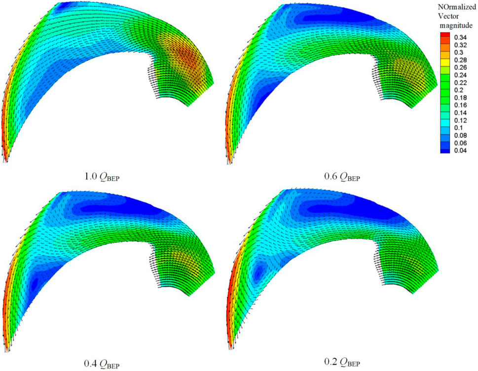
FIGURE 2. Phase-averaged in-plane relative velocity.
It is of particular interest to observe the mean TKE distribution of the velocity field as it is the component responsible for the total energy distribution of injected momentum over the flow field. Figure 3 shows the normalized phase-averaged TKE distributions for different flow rates. Because of the limitations of 2-D measurements, the phase-averaged TKE is calculated through fluctuating components of velocity as shown below:
FIGURE 3. Normalized phase-averaged TKE distributions.
As shown in Figure 3, a global view on the flow field shows that the high TKE values are observed at the passage inlet and outlet, which is consistent with Pedersen (2000). For the flow rate 1.0 QBEP, the high TKE area is located at the passage outlet, which is probably due to the “jet-wake” phenomenon. In addition, compared with other flow rates, the maximum value of TKE is the smallest when the flow rate is 1.0 QBEP due to the relatively uniform flow in the flow channel. For the part load flow rates, high TKE values at the passage inlet near the suction side become maximum, and the other turbulence sheet with less TKE can be observed at the middle of the passage outlet. For the flow rate 0.6 QBEP, flow instability causes blockage at the inlet, making the inlet fluid accelerate, causing a larger shock effect at the inlet, and therefore, generating the maximum turbulent energy. As the flow rate decreases, the flow velocity at the inlet decreases gradually due to the increase of the inlet blockage. Therefore, the maximum value of TKE in the passage decreases gradually. In addition, the deterioration of the internal flow field causes a gradual increase in the area with high TKE values. The high value area located at the inlet extends toward the pressure side, and the high value area located at the outlet extends toward the pressure side, the suction side, and the inlet direction, respectively.
According to the distribution characteristics of the relative phase-averaged velocity and TKE field, four points (marked with a black dot in Figure 1B) are selected for velocity spectrum analysis. Points 1 and 3 are located in the high TKE values area, and points 2 and 4 are located in the core area of the two vortexes, respectively. For this analysis the fast Fourier transformation (FFT) was used within a MATLAB 2014 algorithm. Because there is no unsteady flow generated at the flow rate of 1.0 QBEP, the spectral analysis is only performed for the flow fields of 0.2 QBEP, 0.4 QBEP, and 0.6 QBEP. Figure 4 reveals that the dominant frequencies at flow rates of 0.6 QBEP, 0.4 QBEP, and 0.2 QBEP are 2.2, 3.3, and 6 Hz, respectively. All PSDs were normalized by the maximum peak amplitude value (for the point 1, at the flow rate of 0.2 QBEP). These frequencies lie in the range of 11–30% of the rotor speed, which is known as a typical propagation speed of a stall cell (Pedersen et al., 2003; Krause et al., 2007). As shown in Figure 4A, for the flow rate of 0.6 QBEP, the second and third peaks at point 2 are at 5.0 and 5.9 Hz, respectively. At point 4, the second peak is at 3.1 Hz, and some other peaks are at 4.0 Hz, 5.0 Hz, and so on, meaning the existence of other second flow structures in the vortex region near the suction and pressure side. The highest peak at point 3 is at 3.1 Hz, the second and third peaks are at 3.28 and 4.8 Hz, respectively. These frequencies do not coincide with the main frequencies but are equal or close to the other frequencies at points 2 and 4, probably due to the mixing of the upstream flow at the outlet. As shown in Figure 4B, for the flow rate of 0.4 QBEP, the second peak at point 2 is at 6.5 Hz. At point 3, the highest peak is at 6.5 Hz, which is consistent with the second peak at point 2. At point 4, the second and third peaks are at 5.7 and 4.0 Hz, respectively. As shown in Figure 4C, for the flow rate of 0.2 QBEP, the highest peaks are at 6.0 Hz at points 1, 2, and 4. But the highest peak for point 3 is at 8.2 Hz. Point 2 has a second peak at 8.1 Hz and a third peak at 6.7 Hz, indicating that the suction side appears to have the small-scale structures.
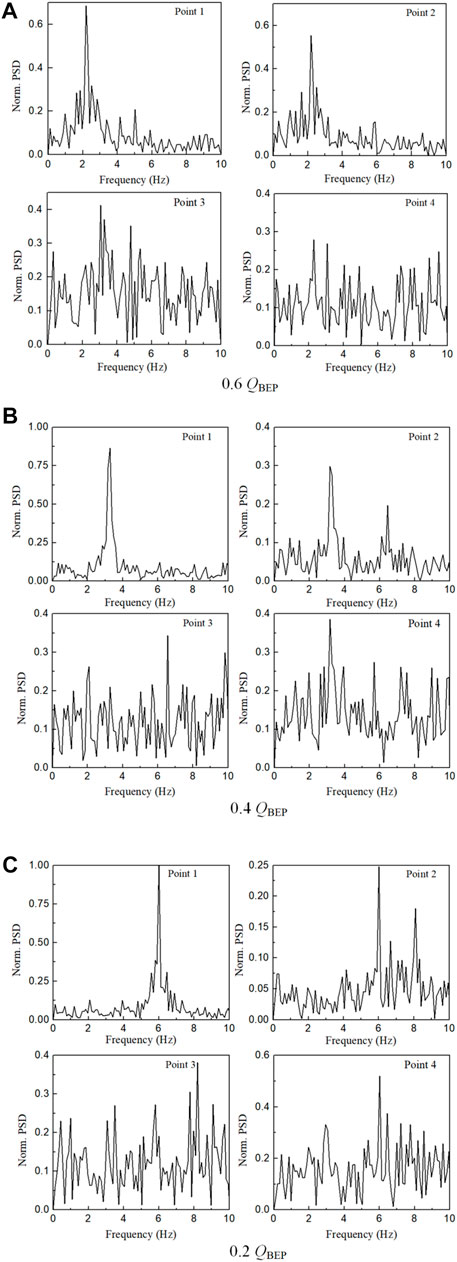
FIGURE 4. Spectra of the velocity fluctuations measured at three points, (A) 0.6 QBEP, (B) 0.4 QBEP, and (C) 0.2 QBEP.
For each flow rate, 200 instantaneous vector fields are used to perform the POD analysis by the POD code in MATLAB. The sensitivity of the POD analysis in relation to the number of the vector fields is studied for the flow rate of 0.4 QBEP. The results obtained for the first six eigenvalues are plotted in Figure 5. The magnitude of the first four largest eigenvalues does not change significantly when the number is larger than 150. This indicates that the number of velocity fields 200 is sufficiently large for providing statistically converged results.
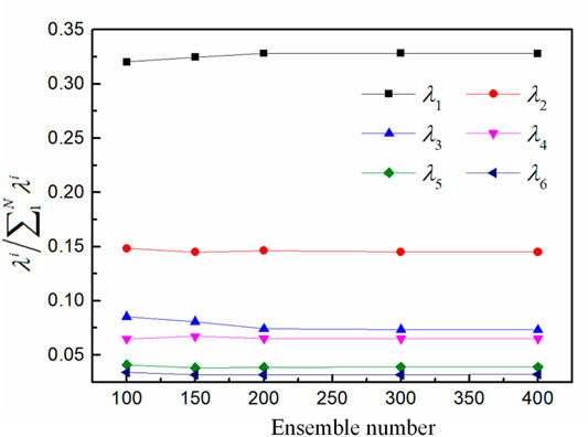
FIGURE 5. Eigenvalue convergence as a function of ensemble size.
The distribution of the relative TKE content
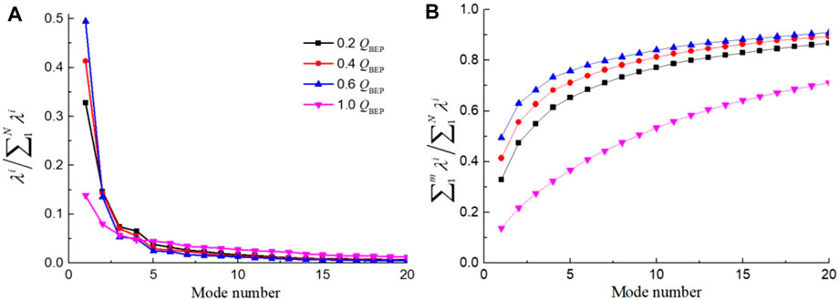
FIGURE 6. (A) Energy contribution of each mode and (B) cumulative energy contents.
TABLE 2. Specific values for the first 10 modes.
Figure 7 shows the vector plots for the first two modes, the contour maps are colored by the vector magnitude which is normalized by Utip. For the flow rate of 1.0 QBEP, the large flow structures are detected at the passage outlet that is near the pressure side for both modes. In addition, the area is consistent with the high TKE area that is shown in Figure 3. Both modes display similar structures as shown in Figure 7, which illustrates the presence of alternate counter-rotating vortexes, reflecting the mutual interaction process occurring between the backflow and the outflow. As for the flow rate of 1.0 QBEP, the fluid in the passage follows the blade very well, thus no large-scale coherent structures in the passage have been observed. However, due to the complexity of the flow in the passage, the low energy fluid has been swept toward the suction side, and the high-energy fluid has been forced toward the pressure side. Therefore, the “jet-wake” structure is taken place at the outlet of the impeller, and the high-energy fluid near the pressure side results in a jet region (Pedersen et al., 2003). The first two modes are the reflection of the mixing of the “jet-wake” (Pedersen et al., 2003), which means that the energy losses are mainly from the “jet-wake” structure for the flow rate of 1.0 QBEP.
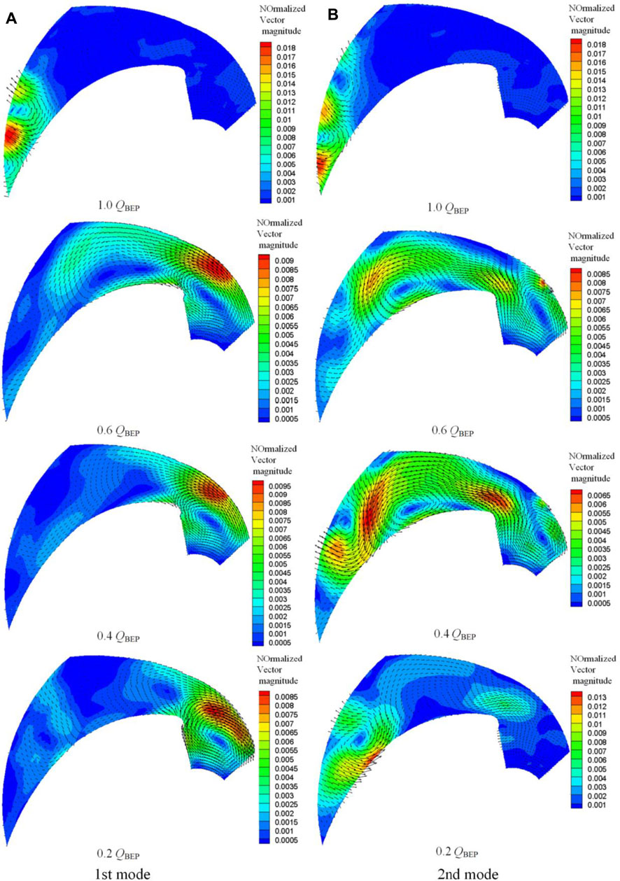
FIGURE 7. The vector plots of the first and second modes for different flow rates. (A) First mode, (B) second mode.
As for the flow rates of 0.2 QBEP to 0.6 QBEP, large flow structures are detected in the passage. For the first mode, at the flow rate of 0.6 QBEP, the kinetic energy is concentrated near the suction side along the passage, a large-scaled anticlockwise vortex structure near the pressure side is observed at the impeller inlet, and an anticlockwise vortex with the same scale is downstream this vortex. The upstream vortex blocks the passage inlet, since the vortex is closer to the pressure side, the fluid near the suction side is accelerated. As the fluid flows downstream, the accelerated fluid bends and forms the second vortex at the leading edge of the pressure side. As the flow rate further decreases to 0.4 QBEP, the kinetic energy is concentrated at the passage inlet, and the downstream vortex disappears, the scale and strength of the upstream vortex increase, due to the stronger blocking effect. When the flow rate decreases to 0.2 QBEP, the upstream vortex turns rotating clockwise, and the flow direction in the passage begins to reverse. Indicating the vortex dynamics is different from that at 0.4 QBEP, and the turbulent kinetic energy is mainly caused by reverse flow. For the flow rates of 0.2 QBEP to 0.6 QBEP, the position of accelerated area is consistent with the high TKE area that is near the passage inlet.
For the second mode, at the flow rate of 0.6 QBEP, the kinetic energy is concentrated at the middle of the passage, a large-scaled clockwise vortex structure near the suction side is observed at the impeller inlet. In addition, an anticlockwise vortex with the same scale near the pressure side downstream the vortex is observed. Both vortexes are induced by the inlet fluid that is near the pressure side. At the passage outlet, a small-scaled vortex is observed downstream the anticlockwise vortex. At the flow rate of 0.4 QBEP, the scales of the two large-scaled vortexes are smaller than that at 0.6 QBEP, but the scale of the vortex near the passage outlet is much larger than that at 0.6 QBEP. At the flow rate of 0.2 QBEP, the kinetic energy is concentrated near the pressure side at the outlet of the passage, and an anticlockwise vortex is detected. For the flow rates of 0.2 QBEP to 0.6 QBEP, the positions of the vortexes that near the outlet are consistent with the high TKE area that nears the passage outlet.
Although there is no classical paired distribution between the first and second modes from the energy content distribution, the flow structures for the first two modes are complementary. To further investigate this observation, the corresponding temporal characteristics are determined. The normalized temporal coefficients (normalized by the maximum value for 0.6 QBEP) of the first two modes are shown in Figure 8A, their normalized frequency spectra (normalized by the maximum peak amplitude value for 0.6 QBEP) are shown in Figure 8B. The cross-correlations between the coefficients are shown in Figure 9. All cross-correlation values are normalized by the same peak amplitude value of cross-correlation values. At the flow rate of 1.0 QBEP, the temporal coefficient for both modes does not exhibit regular variation, and no prominent spectral peak has been found, meaning that no regular vortex shedding persists. Therefore, the structures in the “jet” region might be small-scale fluctuations, or the vortex shedding processes could not be resolved due to the limited time resolution. For the sake of simplicity, the temporal coefficients, the frequency, and the spectra cross-correlations are not shown in the figures.
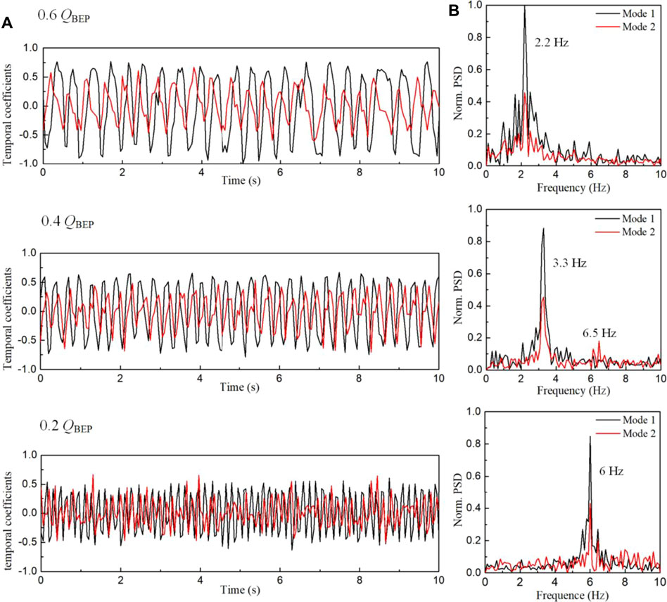
FIGURE 8. Temporal characteristics of mode 1 and mode 2. (A) Temporal coefficients of the first two modes; (B) FFT distribution of the first two modes.
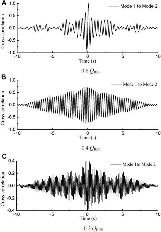
FIGURE 9. Cross-correlation between the first mode and the second mode. (A) 0.6 QBEP, (B) 0.4 QBEP, (C) 0.2 QBEP.
At the flow rate of 0.6 QBEP, the temporal coefficients for the first two modes have the same variation properties except that the variation strength for the second mode is smaller than that for the first mode, and the cross-spectrum showed that the two modes have 0.2 s time lag led by the second mode. Furthermore, a well-defined peak frequency for both modes corresponding to 2.2 Hz is identified. This is consistent with the frequency of stall cell described in Section 3.1. The distinct single peak indicates that there is a single flow phenomenon described by the first two modes at the flow rate of 0.6 QBEP. All the above temporal characteristics for the first and second modes display excellent matches, indicating that the first two modes are different phases of the stall phenomenon.
At the flow rate of 0.4 QBEP, the matching degree for the two modes is smaller than that at 0.6 QBEP. The variation properties of temporal coefficient for the two modes are different; a distinct single peak is identified at 3.3 Hz for the first mode, whereas for the second mode, two peaks are identified, the dominant peak occurs at 3.3 Hz and the other peak occurs at 6.5 Hz with a small amplitude. Furthermore, the cross-spectrum showed less correlation between the two modes. The frequency 3.3 Hz is consistent with the frequency of the stall cell described in Section 3.1. In addition the frequency of 6.5 Hz is consistent with the frequency corresponding to the highest peak of point 3 in Section 3.1. From the vector plots of mode 2 as shown in Figure 7B, the position of point 3 is exactly in the small-scale vortex area at the outlet. Therefore, it can be concluded that the frequency of this small-scale vortex structure is 6.5 Hz. In addition, the second peak of point 2 is also at 6.5 Hz, so it can be inferred that this small-scale vortex is caused by the backflow structure that is induced by the suction side vortex at the outlet. It is precisely because of this small-scale vortex structure that the correlation between the first mode and the second mode is reduced. However, they still mainly reflect the characteristics of the stall phenomenon.
At the flow rate of 0.2 QBEP, the flow structures become more complex, the vector plots and temporal coefficients do not show obvious correlation between the two modes. But the spectral peaks for the two modes both correspond to 6 Hz, the cross-spectrum also shows some correlations between the two modes, suggesting the possibility of limited matches between the two modes.
Figure 10 shows the vector plots for the third and fourth modes. The kinetic energy at different flow rates is concentrated at the passage outlet, and the flow structures are very similar to the first and second modes at 1.0 QBEP, indicating that both the third and fourth modes mainly reflect the characteristics of the ‘jet-wake’ structures. The flow structures extend toward the suction side along the outlet with the decrease of flow rate. For all the flow rates, the distributions of temporal coefficients and cross-spectrum between the third and fourth modes show that there is no obvious correlation between them. Therefore, only the frequency spectra are presented in Figure 11. The frequency spectra distributions are very noisy and multiple peaks at relatively low amplitudes can be observed. The peak frequency situations are also very intriguing. At the flow rate of 0.6 QBEP, the peak frequencies ranked in terms of amplitudes are detected at 3.06, 5.24, 7.32, and 4.0 Hz for the third mode, and 3.82, 8.4, 5.4, and 3.06 Hz for the fourth mode. At the flow rate of 0.4 QBEP, the peak frequencies occur at 4.26, 6.33, and 8.1 Hz for the third mode and 3.25, 2, 6.5, and 5.5 Hz for the fourth mode. While at the flow rate of 0.2 QBEP, the peak frequencies ranked in terms of amplitudes are detected at 6.0, 3.5, 8.1, and 2.1 Hz for the third mode, 6.0 and 8.2 Hz for the fourth mode. In addition, some of these frequencies coincide with those detected in Section 3.1. This suggests that at the outlet, the interaction between the upstream flow structure and the outlet flow structure creates the ‘jet-wake’ structures.
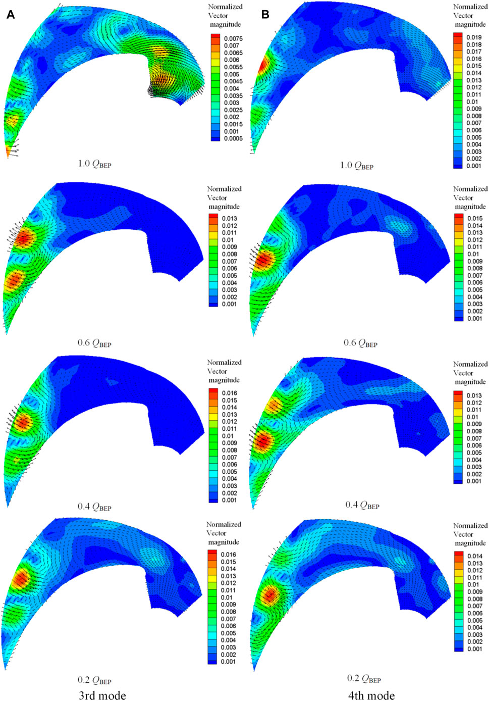
FIGURE 10. The vector plots of the third and fourth modes for different flow rates. (A) Third mode, (B) fourth mode.
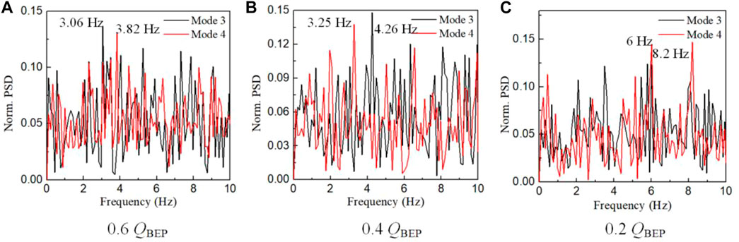
FIGURE 11. FFT distribution of the third mode and the fourth mode. (A) 0.6 QBEP, (B) 0.4 QBEP, (C) 0.2 QBEP.
Figures 12–14 show the vector plots, the temporal frequency spectra, and the cross-correlations between the coefficients for the fifth and sixth modes. At the flow rates of 1.0 QBEP and 0.2 QBEP, the kinetic energy is concentrated at the outlet of the passage, very similar to the “jet-wake” structures, and no obvious peak can be identified for their frequency spectra. Therefore, the results for the flow rates of 0.6 QBEP and 0.4 QBEP are analyzed. At the flow rate of 0.6 QBEP, the kinetic energy for both modes is almost evenly distributed in the whole passage, and three large-scale vortexes can be seen for both modes. In addition, there are some other small-scale structures. For the frequency spectra, the maximum amplitude peaks are distinct and occur at 5.0 Hz for both the fifth and sixth modes. The cross-spectrum shows that the two modes have 0.1 s time lag led by the sixth mode. So that the dominant structures that are described by the two modes represent the same flow phenomenon, we introduce the passage vortexes. The frequency about 5.0 Hz is consistent with the frequency corresponding to the second peak of point 1 and the third peak of points 2 and 4 that were detected in Section 3.1, indicating that the passage vortexes are induced by the stall cell. At the flow rate of 0.4 QBEP, the main flow structures for both modes are also passage vortexes in the passage, but the energy in the outlet area is more concentrated. The frequency spectrum for both modes is also very similar. The maximum amplitude peaks for both modes occur at 6.5 Hz, which is also consistent with the frequency corresponding to the second peak of point 2 and the highest peak of point 3 that were detected in Section 3.1. But their cross-spectrum shows that their correlation decreases a lot. This is due to the appearance of the flow structures corresponding to the next highest peaks: 6.45 and 6.78 Hz correspond to the fifth and sixth modes. This means that the dominance of passage vortexes has been affected by the passage outlet structures. For the seventh mode, the vector plots exhibit smaller and irregular structures. In addition, no obvious peak can be identified for their frequency spectra, too. After the seventh mode, the structures of the higher modes become increasingly random and irregular; the details will not be repeated for the sake of brevity.
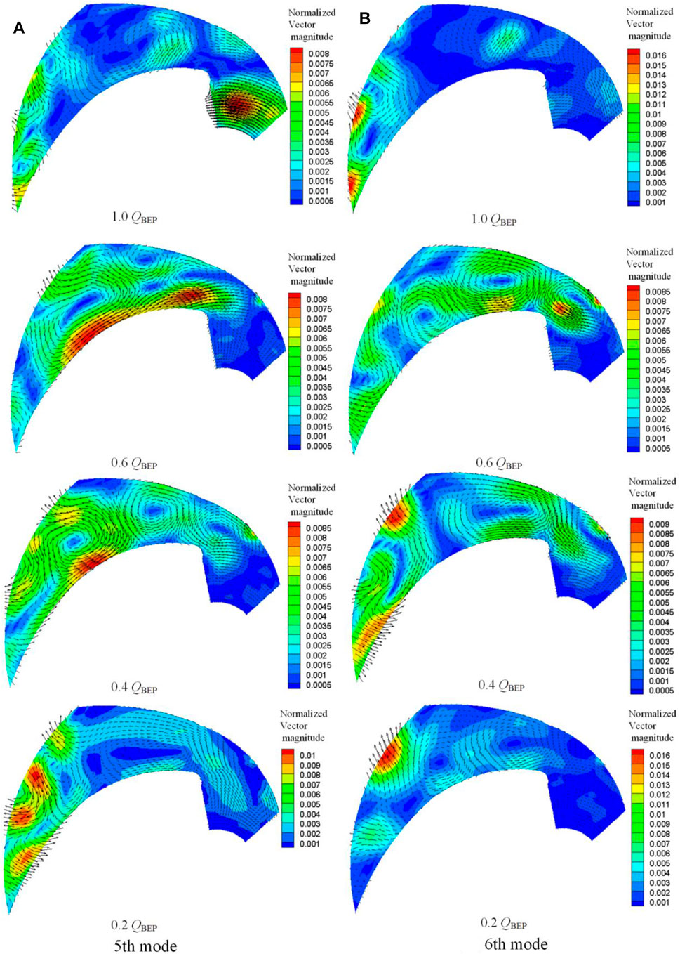
FIGURE 12. The vector plots of the fifth and sixth modes for different flow rates. (A) Fifth mode, (B) sixth mode.

FIGURE 13. FFT distribution of the fifth mode and the sixth mode. (A) 0.6 QBEP, (B) 0.4 QBEP.
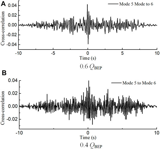
FIGURE 14. Cross-correlation between the fifth mode and sixth mode. (A) 0.6 QBEP, (B) 0.4 QBEP,
Figure 15 shows the reconstructed vector plots using mean velocity and a few lower modes at an arbitrary time at 0.6 QBEP and 1.0 QBEP. At the flow rate of 0.6 QBEP, it is evident that the first two modes are sufficient to capture the largest-scale vortex which has been marked with a red rectangle in Figure 15A. The general structure of the other two vortexes (also marked with a red rectangle) can also be described, but their shapes and scales are significantly different from the raw flow field. As the number of modes considered in POD flow reconstruction increases, the structure of the two vortexes is closer to the raw flow field. When the first seven modes are used, the other two vortexes are basically the same in scale as those in the raw flow field, except for their different shapes. In addition, the flow reconstructed from 20 modes appears identical to the raw data in terms of vector plots. At this time, the energy occupied by the first 20 modes is more than 90% of the total energy. This is another indication that the chosen sample size for the number of flow fields is adequate. In addition, the large-scale structure in the flow field can be well displayed by the first seven modes, which means that the coherent structures in the flow field are mainly composed of the stall structure at the inlet, the “jet wake” structure at the outlet, and the passage vortex structure in the passage. Therefore, during the design of centrifugal pumps, it is suggested to consider suppressing these three types of flow structures, especially the stall structure caused by inlet blockage. This can provide guidance for the design of centrifugal pumps.
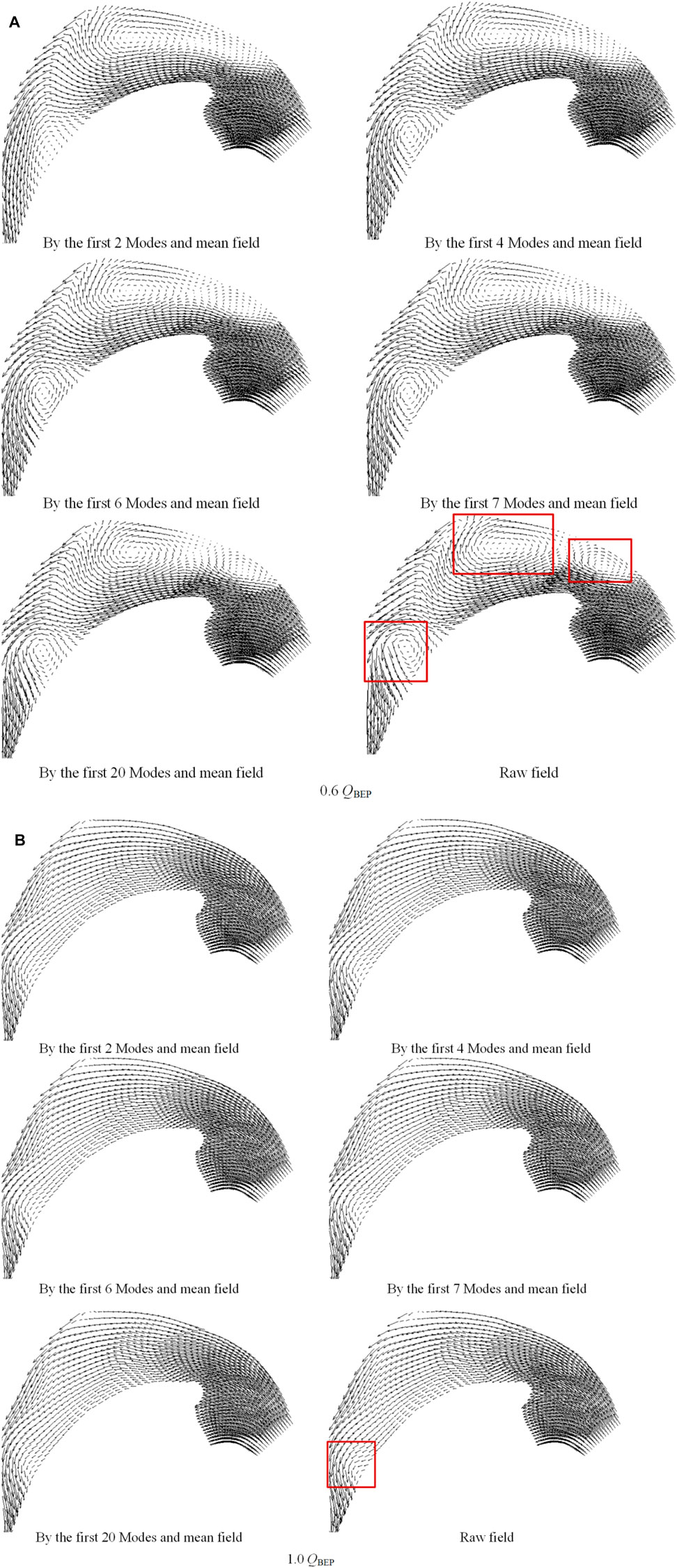
FIGURE 15. Comparison of vector plots between the raw and reconstructed fields. (A) 0.6 QBEP, (B) 1.0 QBEP.
At the flow rate of 1.0 QBEP, the deviation trend of the fluid from the pressure blade near the outlet is captured by the first two modes. As the number of modes considered in POD flow reconstruction increases, the deviation degree of the fluid increases slowly (the deviation area has been marked with a red rectangle in Figure 15B), and the flow structure is closer to the raw flow field. When the flow is reconstructed from 20 modes, the deviation degree is obviously smaller than that of the raw field. At this time, the energy occupied by the first 20 modes is 71.2% of the total energy. This means that more energy is allocated to higher-order modes when the flow field is without a large-scale flow structure. Therefore, the flow field reconstructed from the first few modes is not enough to express the flow characteristics.
The unsteady behavior of flow structures in a centrifugal pump is investigated by means of TR-PIV measurements. Four cases with different flow rates, e.g., 0.2 QBEP, 0.4 QBEP, 0.6 QBEP, 1.0 QBEP, are chosen for investigation. The POD method is employed to decouple and reconstruct the coherent structures of flow fields. The main conclusions can be drawn as follows:
1) The mean results show that the decrease of the relative velocity and the deviation to the suction side of the inlet fluid are the main causes of unstable flow. The TKE statistical results show that at the flow rate of 1.0 QBEP, the highest TKE value area is located at the passage outlet due to the “jet-wake” phenomenon; for the part load flow rates, the highest TKE values are concentrated at the passage inlet near the suction side due to the larger shock effect of the inlet flow. The velocity spectra results show that the dominant frequencies for part load flow rates reveal a typical propagation speed of a stall cell.
2) For the best efficiency point (1.0 QBEP), the fluid follows the blade contour very well. In addition, the main POD modes show that the coherent structures are located at the passage outlet and are shown as alternate counter-rotating vortexes, which is due to the mixing of the “jet-wake” structures.
3) For the medium part-load condition (0.4 QBEP to 0.6 QBEP), the first and second modes are found to be associated in pairs corresponding to the stall cells. However, the flow structures of the first two modes change as the flow rate decreases, resulting in the weakening of the correlation between the first and second modes, and the increase of stall cell frequency. The third and fourth modes are found to be associated with the ‘jet-wake’ structures; some of the frequencies for the third and fourth modes are consistent with the frequencies of the velocity spectrums, indicating that the interaction between the upstream flow structure and the outlet flow structure creates the “jet-wake” structures. The fifth and sixth modes are found to be associated with the passage vortexes, and the passage vortexes are induced by the stall cell.
4) For the extreme part-load condition (0.2 QBEP), the characteristics of the stall cells are different from that at medium part-load condition: the stall cells shown in the first and second modes are reverse flow, the rotation directions of the stall cells are opposite to that of the medium part-load condition, indicating the turbulent kinetic energy of the internal flow is mainly caused by the reverse flow; furthermore, the third to sixth modes are all displayed as jet-wake characteristics.
5) POD can reconstruct the flow structures when large-scale flow structures appear in the flow field. The large-scale structures can be reconstructed by the first two high-energy modes and the phase-averaged approach; the reconstruction of the smaller scale structures required at least six POD modes when a large-scale coherent structure appears. This suggests that most of the turbulent kinetic energy is manifested in the first few modes; therefore, the inlet region and outlet region should be optimized to suppress the generation of stall cells and “jet-wake” structures.
The original contributions presented in the study are included in the article/Supplementary Material, Further inquiries can be directed to the corresponding author.
B.C.: Writing-original draft preparation, MATLAB programming, visualization. X.L.: Conceptualization, data curation, investigation, methodology. Z.Z.: Conceptualization, supervision, writing—review and editing.
This work was supported by the National Natural Science Foundation of China (Grant Nos. 51806197, U1709209), the Natural Science Foundation of Zhejiang Province (No. LY20E060006). Key Research and Development Program of Zhejiang Province (Grant No. 2021C05006). Top-notch Talent Support Program of Zhejiang Province (Grant No. 2019R51002). The Fundamental Research Funds of Zhejiang Sci-Tech University (Grant No. 2021Q017). The supports are gratefully acknowledged.
The authors declare that the research was conducted in the absence of any commercial or financial relationships that could be construed as a potential conflict of interest.
All claims expressed in this article are solely those of the authors and do not necessarily represent those of their affiliated organizations, or those of the publisher, the editors, and the reviewers. Any product that may be evaluated in this article, or claim that may be made by its manufacturer, is not guaranteed or endorsed by the publisher.
The supports are gratefully acknowledged.
Arun Shankar, V. K., Umashankar, S., Paramasivam, S., and Hanigovszki, N. (2016). A Comprehensive Review on Energy Efficiency Enhancement Initiatives in Centrifugal Pumping System. Appl. Energ. 181, 495–513. doi:10.1016/j.apenergy.2016.08.070
Bozorgasareh, H., Khalesi, J., Jafari, M., and Gazori, H. O. (2021). Performance Improvement of Mixed-Flow Centrifugal Pumps with New Impeller Shrouds: Numerical and Experimental Investigations. Renew. Energ. 163, 635–648. doi:10.1016/j.renene.2020.08.104
Ghorani, M. M., Sotoude Haghighi, M. H., Maleki, A., and Riasi, A. (2020). A Numerical Study on Mechanisms of Energy Dissipation in a Pump as Turbine (PAT) Using Entropy Generation Theory. Renew. Energ. 162, 1036–1053. doi:10.1016/j.renene.2020.08.102
Han, Y., and Tan, L. (2020). Dynamic Mode Decomposition and Reconstruction of Tip Leakage Vortex in a Mixed Flow Pump as Turbine at Pump Mode. Renew. Energ. 155, 725–734. doi:10.1016/j.renene.2020.03.142
Holmes, P. J., Lumley, J. L., Berkooz, G., Mattingly, J. C., and Wittenberg, R. W. (1997). Low-dimensional Models of Coherent Structures in Turbulence. Phys. Rep. 287, 337–384. doi:10.1016/s0370-1573(97)00017-3
Kaupert, K. A., and Staubli, T. (1999). The Unsteady Pressure Field in a High Specific Speed Centrifugal Pump Impeller-Part I: Influence of the Volute. J. Fluid Eng. 121 (3), 621–626. doi:10.1115/1.2823514
Kaupert, K. A. (1999). The Unsteady Pressure Field in a High Specific Speed Centrifugal Pump Impeller—Part II: Transient Hysteresis in the Characteristic. J. Fluid Eng. 121 (3), 3558–3565. doi:10.1115/1.2823515
Keller, J., Blanco, E., Barrio, R., and Parrondo, J. (2014). PIV Measurements of the Unsteady Flow Structures in a Volute Centrifugal Pump at a High Flow Rate. Exp. Fluids 55 (10), 1820. doi:10.1007/s00348-014-1820-7
Krause, N., Pap, E., and Thevenin, D. (2007). Influence of the Blade Geometry on Flow Instabilities in a Radial Pump Elucidated by Time-Resolved Particle-Image Velocimetry. Proc. ASME Turbo Expopower Land, Sea, Air 6, 1659–1668. doi:10.1115/gt2007-27455
Krause, N., Zähringer, K., and Pap, E. (2005). Time-resolved Particle Imaging Velocimetry for the Investigation of Rotating Stall in a Radial Pump. Exp. Fluids 39 (2), 192–201. doi:10.1007/s00348-005-0935-2
Li, D., Wang, H., Qin, Y., Wei, X., and Qin, D. (2018). Numerical Simulation of Hysteresis Characteristic in the Hump Region of a Pump-Turbine Model. Renew. Energ. 115, 433–447. doi:10.1016/j.renene.2017.08.081
Li, J., Liu, J., Pei, J., Mohanarangam, K., and Yang, W. (2018). Experimental Study of Human thermal Plumes in a Small Space via Large-Scale TR PIV System. Int. J. Heat Mass Transfer 127, 970–980. doi:10.1016/j.ijheatmasstransfer.2018.07.138
Li, W., Ji, L., Li, E., Ramesh, A., and Zhou, L. (2020). Numerical Investigation of Energy Loss Mechanism of Mixed-Flow Pump under Stall Condition. Renew. Energ. 167 (9), 740–760. doi:10.1016/j.renene.2020.11.146
Li, W., Li, E., Ji, L., Zhou, L., Shi, W., and Zhu, Y. (2020). Mechanism and Propagation Characteristics of Rotating Stall in a Mixed-Flow Pump. Renew. Energ. 153, 74–92. doi:10.1016/j.renene.2020.02.003
Li, X., Chen, B., Luo, X., and Zhu, Z. (2020). Effects of Flow Pattern on Hydraulic Performance and Energy Conversion Characterisation in a Centrifugal Pump. Renew. Energ. 151 (5), 475–487. doi:10.1016/j.renene.2019.11.049
Li, X., Chen, H., Chen, B., Luo, X., Yang, B., and Zhu, Z. (2020). Investigation of Flow Pattern and Hydraulic Performance of a Centrifugal Pump Impeller through the PIV Method. Renew. Energ. 162, 561–574. doi:10.1016/j.renene.2020.08.103
Lim, H. D., Ding, J., Shi, S., and New, T. H. (2019). Proper Orthogonal Decomposition Analysis of Near-Field Coherent Structures Associated with V-Notched Nozzle Jets. Exp. Therm. Fluid Sci. 112, 109972.
Lumley, J. L. (1967). The Structure of Inhomogeneous Turbulent Flows. J. Comput. Chem. 790, 166–178.
Pedersen, N. (2000). Experimental Investigation of Flow Structures in a Centrifugal Pump Impeller Using Particle Image Velocimetry Technical University of Denmark. Technical University of Denmark.
Pedersen, N., Larsen, P. S., and Jacobsen, C. B. (2003). Flow in a Centrifugal Pump Impeller at Design and Off-Design Conditions-Part I: Particle Image Velocimetry (PIV) and Laser Doppler Velocimetry (LDV) Measurements. J. Fluid Eng. 125, 61–72. doi:10.1115/1.1524585
Santolaria Morros, C., Fernández Oro, J. M., and Argüelles Díaz, K. M. (2011). Numerical Modelling and Flow Analysis of a Centrifugal Pump Running as a Turbine: Unsteady Flow Structures and its Effects on the Global Performance. Int. J. Numer. Meth. Fluids 65 (5), 542–562. doi:10.1002/fld.2201
Semlitsch, B., and Mihăescu, M. (2016). Flow Phenomena Leading to Surge in a Centrifugal Compressor. Energy 103 (C), 572–587. doi:10.1016/j.energy.2016.03.032
Shi, G., Liu, Z., Xiao, Y., Li, H., and Liu, X. (2020). Tip Leakage Vortex Trajectory and Dynamics in a Multiphase Pump at Off-Design Condition. Renew. Energ. 150, 703–711. doi:10.1016/j.renene.2020.01.024
Sirovich, L. (1987). Turbulence and the Dynamics of Coherent Structures. I. Coherent Structures. Quart. Appl. Math. 45, 561–571. doi:10.1090/qam/910462
Tan, L., Yu, Z., Xu, Y., Liu, Y., and Cao, S. (2017). Role of Blade Rotational Angle on Energy Performance and Pressure Fluctuation of a Mixed-Flow Pump. Proc. Inst. Mech. Eng. Part. A. J. Power Energ. 231, 227–238. doi:10.1177/0957650917689948
Tang, Z., Fan, Z., Ma, X., Jiang, N., Wang, B., Huang, Y., et al. (2020). Tomographic Particle Image Velocimetry Flow Structures Downstream of a Dynamic Cylindrical Element in a Turbulent Boundary Layer by Multi-Scale Proper Orthogonal Decomposition. Phys. Fluids 32 (12), 125109. doi:10.1063/5.0026955
Wernet, M. P. (2000). Application of DPIV to Study Both Steady State and Transient Turbomachinery Flows. Opt. Laser Technol. 32 (7-8), 497–525. doi:10.1016/s0030-3992(00)00090-6
Westra, R. W., Broersma, L., Andel, K. V., and Kruyt, P. (2010). PIV Measurements and CFD Computations of Secondary Flow in a Centrifugal Pump Impeller. ASME J. Fluids Eng. 132 (6), 061104. doi:10.1115/1.4001803
Xia, L. S., Cheng, Y. G., Zhang, X. X., and Yang, J. D. (2014). Numerical Analysis of Rotating Stall Instabilities of a Pump- Turbine in Pump Mode. IOP Conf. Ser. Earth Environ. Sci. 22 (3), 032020. doi:10.1088/1755-1315/22/3/032020
Yang, S. Q., Wang, Y. H., Yang, M., Song, Y. W., and Yan, H. (2019). POD-based Data Mining of Turbulent Flows in Front of and on Top of Smooth and Roughness-Resolved Forward-Facing Steps. IEEE Access. 7 (1), 18234–18255.
Zhang, L., Wang, C., Zhang, Y., Xiang, W., He, Z., and Shi, W. (2021). Numerical Study of Coupled Flow in Blocking Pulsed Jet Impinging on a Rotating wall. J. Braz. Soc. Mech. Sci. Eng. 43, 508. doi:10.1007/s40430-021-03212-0
Zhang, N., Zheng, F., and Liu, X. (2020). Unsteady Flow Fluctuations in a Centrifugal Pump Measured by Laser Doppler Anemometry and Pressure Pulsation. Phys. Fluids 32 (12), 108–125. doi:10.1063/5.0029124
Zhou, T., Zhong, S., and Fang, Y. (2021). Trailing-edge Boundary Layer Characteristics of a Pitching Airfoil at a Low Reynolds Number. Phys. Fluids 33 (3), 033605. doi:10.1063/5.0039416
A eigenvector
b blade height, mm
D diameter, mm
fBP rotation frequency of the impeller
M the number of spatial nodes in a single snapshot
QBEP design flow rate, m3/h
r radius, mm
U absolute velocity, m/s
u horizontal velocity component
Utip blade tip speed
V the matrix of velocity
v vertical velocity component
W relative velocity, m/s
Z number of blades
β blade angle, °
λ eigenvalue
1 parameters are related to fluctuating value impeller inlet
1 parameters are related to fluctuating value impeller inlet
2 impeller outlet
Keywords: TR-PIV, centrifugal pump, POD, coherent structure, energy loss
Citation: Chen B, Li X and Zhu Z (2022) Time-Resolved Particle Image Velocimetry Measurements and Proper Orthogonal Decomposition Analysis of Unsteady Flow in a Centrifugal Impeller Passage. Front. Energy Res. 9:818232. doi: 10.3389/fenrg.2021.818232
Received: 19 November 2021; Accepted: 21 December 2021;
Published: 31 January 2022.
Edited by:
Enhua Wang, Beijing Institute of Technology, ChinaCopyright © 2022 Chen, Li and Zhu. This is an open-access article distributed under the terms of the Creative Commons Attribution License (CC BY). The use, distribution or reproduction in other forums is permitted, provided the original author(s) and the copyright owner(s) are credited and that the original publication in this journal is cited, in accordance with accepted academic practice. No use, distribution or reproduction is permitted which does not comply with these terms.
*Correspondence: Xiaojun Li, bGl4akB6c3R1LmVkdS5jbg==
Disclaimer: All claims expressed in this article are solely those of the authors and do not necessarily represent those of their affiliated organizations, or those of the publisher, the editors and the reviewers. Any product that may be evaluated in this article or claim that may be made by its manufacturer is not guaranteed or endorsed by the publisher.
Research integrity at Frontiers
Learn more about the work of our research integrity team to safeguard the quality of each article we publish.