Fault Location with High Precision of Flexible DC Distribution System Using Wavelet Transform and Convolution Neural Network

Though flexible DC distribution system (FDCDS) is becoming a new hotspot in power systems lately because of the rapid development of power electronic devices and massive use of renewable energy, the failure to realize accurate fault location with high precision restricts its further application. Thus, a novel precise pole-to-ground fault location method of FDCDS based on wavelet transform (WT) and convolution neural network (CNN) is proposed in this paper for the limitation on the number of measuring points and high difficulty in extracting characteristics of FDCDS. The fault voltage signal is decomposed with multi-resolution by discrete wavelet transform (DWT), and then the transient energy function is constructed to select the frequency bands containing rich fault characteristics for signal reconstruction. The reconstructed signal forms two-dimensional time-frequency images through continuous wavelet transform (CWT), which are used as the input of CNN classifier after image enhancement to form the mapping relation between the fault feature and fault position using the powerful generalization ability of CNN, so as to complete fault location with high precision. The sample data on PSCAD/EMTDC verifies the accuracy and reliability of the proposed method, which can achieve fault location with positioning precision of 30 m. The proposed method overcomes the influence of the control strategy of the converter and the number of input capacitors of the bridge arm in the time-domain analysis, and still has strong robustness in the case that FDCDS is connected with many distributed generations (DGs) with output fluctuation. Furthermore, four other methods for fault location as comparisons are given to reflect the validity and anti-interference ability of proposed methods in various noises.

Introduction

FLEXIBLE DC distribution system (FDCDS) is becoming a new developing direction of power system due to its advantages of being suitable for DGs multi-point access and asynchronous interconnection (Mohsenian-Rad and Davoudi, 2014). FDCDS based on Modular Multilevel Convertor (MMC) has been widely applied in many demonstration projects. However, the characteristics of FDCDS are different from traditional AC distribution networks in that the complex control strategies and dense branches, which make it difficult to directly apply the protection principle and scheme of AC network to the fault detection and location of FDCDS, thus, its large-scale engineering application is limited (Liu et al., 2020), (Huang et al., 2011). When a short-circuit fault occurs, the voltage drops rapidly and the current rises fast, seriously endangering the safe and stable operation of the power system, so it is necessary to quickly identify, locate the fault, and remove it.

Nowadays, the fault location method for FDCDS can be roughly divided into two approaches, the first is that the fault characteristics are analyzed and the fault distance equation is solved to obtain the fault location. The second approach is to utilize an intelligent algorithm to locate the fault.

Copied from the traditional line protection method of high voltage direct current transmission (HVDC) (Zheng et al., 2021), (Tang et al., 2019), three ways of line protection are introduced to FDCDS, which are the travelling wave method, the active injection method, and the fault analysis method (Dhar et al., 2018). Lin et al. (2017) proposed extracting travelling waves by using wavelet modulus maximum, which only needs to record the first time of travelling waves arriving at each terminal and select the nearest fault occurring time (FOT) to achieve location. Though the method performs better than traditional travelling wave method, it is restricted by the blind zone and the number of the measuring points. Additional signals are injected by the injection device and further detected to obtain additional signals to calculate the fault distance in the active injection method (Christopher et al., 2011), (Mohanty et al., 2016). But this method is strict with the topological structure of the network and is easily affected by noise. Apart from these two, most of the current research on fault location of FDCDS is based on the analysis of its fault characteristics and the corresponding algorithm is introduced to construct the relationship of fault location and transient component (Wang et al., 2019; Li et al., 2020; Yan et al., 2020; Yuan et al., 2020). Except the basic fault feature analysis, the fault’s modal parameters and time domain characteristics are also utilized to the fault location. Tawfik and Morcos (2005) use the Prony method to extract modal information of fault current waveform which is strongly relevant to the fault location. But the fundamental frequency component’s damping coefficients will cause influence on the accuracy of the location. On this basis, the linear relation between fault location and damping coefficient is established in the Prony method to locate the fault, which eliminates the effect of load fluctuation and fault types. However, the influence of transient resistance is not considered (Gou and Owusu, 2008). References (Jia et al., 2020) and (He et al., 2014) analyze the relationship between the frequency feature of fault voltage or current and fault distance, but it also means that the selection of frequency range will have an impact on the final positioning result.

The development of intelligent algorithm provides a novel solution for fault location, such as expert system (Lee et al., 2000), fuzzy algorithm (Huisheng Wang and Keerthipala, 1998), improved genetic algorithm (Li et al., 2012), and deep learning (Guomin et al., 2018). Both bionic algorithm and deep learning based on neural network have the problems in convergence performance and easily falling into local optimal when facing complex situations, hence, the directions to increase the accuracy of methods are divided into two categories: enhancing the characteristics information of sample data and multiple algorithms fusion. The time delay, characteristic frequency, energy attenuation, and high-frequency energy via the Hilbert-Huang Transform (HHT) are used as the input of support vector regression (SVR) to get fault distance, then the parameters of the model is optimized by the bat algorithm (BA) (Hao et al., 2018). Based on the feature extraction ability of the convolution neural network (CNN), reference (Liang et al., 2020) adopts the improving pooling model and the result shows the method improves the accuracy greatly.

In general, the current fault location problems of FDCDS are mainly reflected in the difficulty to extract fault features. Especially the location accuracy is easily affected by noise and converter, which cause the low location precision. Therefore, the main contribution of this paper is a novel pole-to-ground fault location method of FDCDS, it can identity fault position with high precision, even under the interference of transient resistance, output fluctuation of DGs, and different noises. In addition, the proposed method eliminates the influence of the converter control strategy and the switching of sub-modules (SMs). Compared with the existing methods, this paper adopts wavelet transform to enhance the sample feature, magnify the sample characteristics, and increase the number of the input data, to solve the problem of difficulty in feature extraction and insufficient feature quantity under the limited fault information. Convolutional neural network is used to mine the mapping relationship between fault features and fault positions to solve the problem of insufficient accuracy of existing algorithms.

Fault Location Method

Fault Analysis

In FDCDS, pole-to-pole faults do great harm to the system and have obvious fault characteristics, most of the current fault location research is focused on pole-to-pole faults. While single-pole faults do not have obvious fault features due to transition resistance, there are few studies on its fault location. In fact, pole-to-ground fault is the fault with the highest frequency, so the fault location of the distribution line for pole-to-ground is mainly studied in this paper. The transient process after short-circuiting mainly can be divided into two processes: SM’s capacitor discharging; the grid side feeds the short-circuit current into the DC system through the bridge-arm reactor and the anti-parallel diode when the DC side’s voltage drops to less than the peak voltage of the AC side. Considering that the fault current rises fast when the fault occurs, which will cause a huge impact on expensive converter equipment, so the SM’s capacitor discharging stage of the transient process is taken to locate the faults in this paper.

Figure 1A shows the discharging circuit of SMs, in which FDCDS converter transformer valve side is grounded, and the current direction has been marked. To analyze the pole-to-ground fault from the fault equivalent loop in Figure 1B, the quantity of the input capacitor and the value of transient resistance need to be considered. But at the fault initial time, the input capacitor of the upper and lower bridge arm is unknown as the SMs are normally switched under the control strategy and transient resistance is also changing, making it difficult to utilize the fault loop to deduce the relationship between voltage (or current) and fault location. But it is clear that the electric data emerged at different fault locations on the line are different, although the relationship between these two cannot be explicitly given by an equation. Therefore, this paper decided to use deep learning and wavelet transform to fit the relationship between fault features and fault locations instead of manual formula derivation.

FIGURE 1

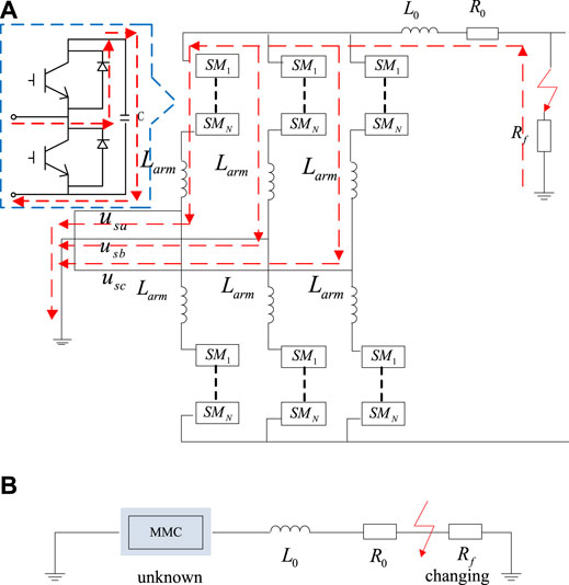
FIGURE 1. Fault analysis. (A) The discharging circuit of SM’s capacitor. (B) Fault equivalent circuit.

Signal Analysis Based WT

Wavelet transform is a time-frequency analysis tool, which can show the amplitude of a signal in a different frequency domain over a period of time. WT mainly includes discrete wavelet transform (DWT) and continuous wavelet transform (CWT). DWT is used to decompose the fault voltage signal into multiple frequency bands in this paper, and then the selected frequency band signals are reconstructed to obtain the reconstructed signals with rich fault features. CWT is applied to the processed signals to generate two-dimensional grayscale images that serve as the inputs of CNN to complete fault location.

The multi-resolution analysis (MRA) is used to decompose the signal in multiple frequency bands, it is applied to DWT to divide signals to approximate component A (t) and detail component D (t), which represent the low and high frequency bands, respectively, and the decomposition tree of DWT-based MRA is shown in Figure 2.

FIGURE 2

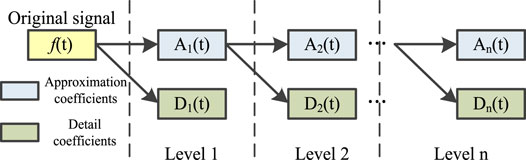
FIGURE 2. The decomposition tree of DWT-based MRA.

If the Fourier transform of function φ (t) satisfies the admissibility condition shown in Equation (1), then φ (t) is called a fundamental wavelet, also known as a mother wavelet function.

$C_{\phi }={\displaystyle \int \frac{{\left|\widehat{\phi }\left(\omega \right)\right|}^2}{\left|\omega \right|}}d\omega <\infty (1)$

The integral transforms of the following formulas are defined as the CWT and DWT based on φ(t).

$CW{T}_x\left(a,b\right)={\left|a\right|}^{\frac{1}{2}}{\displaystyle \int f\left(x\right)}\overline{\phi }\left(\frac{x-a}{b}\right)dx,f\left(x\right)\in L^2\left(R\right)(2)$

$DW{T}_x\left(u,v\right)={\left|a_0^u\right|}^{\frac{1}{2}}{\displaystyle \sum _{v}f\left(x\right)}\phi \left(\frac{x-v{a}_0^u{b}_0}{a_0^u}\right)(3)$

where a is a scale parameter, b is a translation parameter in CWT. For DWT, a₀^uis a scale parameter and va₀^ub₀ is a translation parameter.

The Structure and Principle of CNN

The typical structure of CNN is depicted in Figure 3. The 2D gray image as input is expanded to the fully connected layer after passing though the convolutional layer (Conv layer) and sub-sampling layer (S layer) and outputs the results via softmax classification. The Conv layer is composed of a 2D image convolution, batch normalization (BN), and Rectified Linear Unit (ReLU) (Gu et al., 2015). The 2D gray value matrix after padding is mapped to the next layer through the convolution kernel. BN is set to prevent gradient explosion. ReLU, as the activation function, effectively solves the problem of gradient dispersion. The two main methods of sub-sampling are maximum pooling (max-pooling) and mean pooling (mean-pooling) (Zhao et al., 2018), and they are mainly used to extract the signal features more finely. Through multi-level non-linear transformation, the neural network would automatically extract and recognize the feature of input set and classify mass data according to the labels.

FIGURE 3

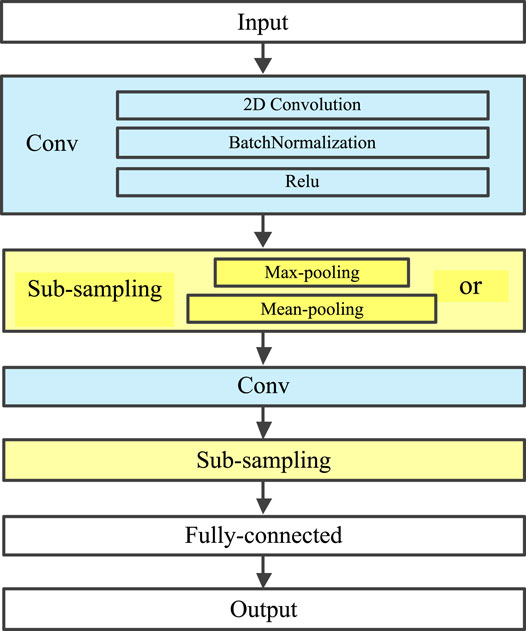
FIGURE 3. The structure of CNN.

A fully connected layer is a one-dimensional vector to store an eigenvector after the Conv layers and S layers. The column vectors are mapped to an output layer, and then the classification results are generated via softmax function, which calculation formula is denoted as Equation (4).

$y_i=\phi \left(v_i\right)=\frac{e^{vi}}{e^{v1}+e^{v2}+e^{v3}+\cdots e^{vM}}=\frac{e^{vi}}{{\displaystyle \sum _{i\in M}{e}^{vk}}}(4)$

where M is the number of the output nodes. According to Equation (4), the sum of the vectors output after the classifier is 1.

CNN neural network training process involves the adjustment of many weights. In order to speed up the training and improve the stability, the concept of “momentum” in physics is introduced (Kim, 2017). In physics, momentum is a concept similar to inertia, which can prevent objects from rapidly changing the motion state. The momentum term is used in weight adjustment to push the weight to adjust to a certain direction to a certain extent, instead of causing immediate changes.

Proposed Method

The proposed method is illustrated in Figure 4, and it is mainly divided into two parts: signal processing based WT and classification based CNN. The main problem to be solved in this paper is fault location with high precision, so it is necessary to extract rich and effective fault features in the signal processing stage. First, DWT-based MRA is used to decompose the signal, and then the transient energy of each frequency band is constructed to select the frequency band where the useful signal is and complete the signal reconstruction. Then, CWT is applied to generate a two-dimensional time-frequency image with rich characteristic information. Apart from signal processing, fault location mainly relies on CNN to process a grayscale image with characteristic information. After initialization and a lot of trainings, the fault location task with high precision can be accurately completed. The following part will explain the feature extraction in signal processing in detail, and the steps of CNN classification will be given in the third part combined with experiments.

FIGURE 4

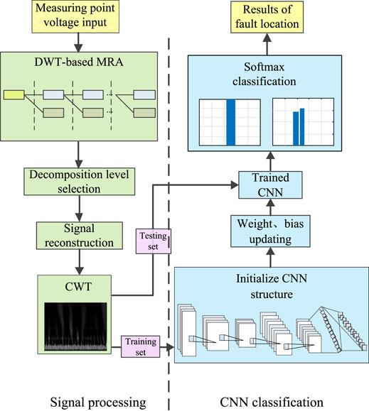
FIGURE 4. The flowchart of the proposed method.

DWT-Based MRA

In wavelet transform, db4 wavelet with good regularity is used as the wavelet basis function. According to Nyquist sampling theorem, the frequency band of the high-filter of each decomposition level is [F_S/2ⁿ⁺¹, F_S/2ⁿ], then [0, F_S/2ⁿ⁺¹] is for low-filter of each level. The principle of signal decomposition is to make the reconstructed signal contain the most unique features as far as possible. If the decomposition level is too little, the feature information and irrelevant information will be overlapped together, affecting the final location results. If the decomposition level is too much, according to the MRA principle, the frequency of decomposition has dropped below 39 Hz after level 8, and there is no need to continue decomposition. So, the decomposition level is set to 8. In the preliminary simulation test process, the sampling rate of 20 kHz is found to be sufficient and brings the right balance between accuracy and speed, guaranteeing high precision of fault location and quick and timely response. So, the original signal is decomposed into 8 frequency bands covering frequencies from 39.163 Hz to 10 kHz. Frequency band after multi-resolution decomposition is shown in Figure 5.

FIGURE 5

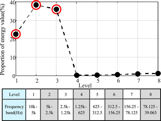
FIGURE 5. Transient energy proportion of each level.

Decomposition Level Selection

To extract effective fault feature information and select the frequency bands where the useful signal is located, define the voltage transient energy E_h as shown in Equation (5), which can reflect the richness of fault characteristics in each frequency band.

$E_h={\displaystyle {\int }_0^T{d}_n{\left(t\right)}^2}dt(5)$

where d_n is a high-filter coefficient, T is integral time. Figure 5 is the ratio of the transient energy of each frequency band to the sum of the energy of the 8 frequency bands when pole-to-ground fault occurs at a distribution line. As can be seen from Figure 5, the energy in the transient process is mainly concentrated in Level 1, 2, and 3 (the frequency band covering from 1.25 to 10 kHz), which indicates that this part of the frequency band contains most of the characteristic information. Therefore, it is more accurate to select the fault information within these three levels to complete the fault location in the next step.

Signal Reconstruction

Signal reconstruction of the frequency band selected in the previous step can effectively eliminate noise interference caused by external factors such as sensors (noise occupies a low proportion of energy). According to Mallat’s algorithm (Mallat, 1989), in multi-resolution decomposition, signals are decomposed via high-pass and low-pass filters, and reconstruction is the convolution of decomposed signals, and the mirror filter banks. Suppose that D⁻¹ is the reconstructed signal of detail coefficient D, the reconstructed signal is denoted as S(t),

$S\left(t\right)=D_1^{-1}\left(t\right)+D_2^{-1}\left(t\right)+D_3^{-1}\left(t\right)(6)$

Figure 6 shows the process of signal reconstruction, in which Figure 6A is the original signal. Figures 6B–E are part of the signal (D1-D4) after decomposition, and it can be clearly seen that the transient energy of signal is mainly concentrated in D1, D2 and D3, D4, and the other bands contain only a small amount of useful information. The decomposition levels D1, D2, and D3 are used to reconstruct a new signal (Figure 6F), which not only can extract the effective feature information, but also can eliminate the noise interference.

FIGURE 6

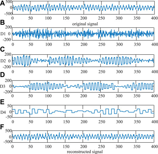
FIGURE 6. Signal reconstruction. (A) original signal (B) detail coefficient D1 (C) detail coefficient D2 (D) detail coefficient D3 (E) detail coefficient D4 (F) reconstructed signal.

Grayscale Image and Image Preprocessing

CWT is applied to the reconstructed signal to generate a two-dimensional time-frequency image (grayscale image) for CNN classifier. In order to enhance the effect of image recognition, the image is preprocessed before the CNN training. Figure 7 is the grayscale image after image enhancement, and the fault features are more obvious. Meanwhile, the noise influence of the reconstructed signal of the selected frequency band is eliminated in this step, and the accuracy of positioning is further improved.

FIGURE 7

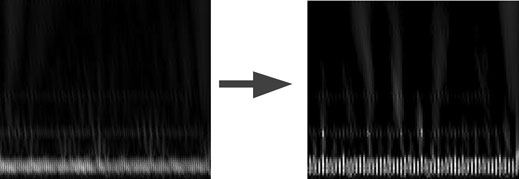
FIGURE 7. Grayscale image and image preprocessing.

Simulation Results

FDCDS Model

A typical FDCDS of 10 kV voltage class (adapted from the demonstration project of flexible DC distribution system in Shenzhen) in Figure 8 is built in PSCAD/EMTDC to verify the reliability and accuracy of the proposed method. The selected topology in this paper is the loop structure, which has the highest power supply reliability and the highest requirements for protection. In addition, the adaptive feature extraction based on transient energy method according to different topologies is adopted in the paper, theoretically applicable to the relatively simple radial structure and other topologies. Cable #1 connects two AC grids (10 kV) through two MMCs (5MVA) that are operated at the constant DC voltage mode and the constant active/reactive power mode to carry out rectifier and inverter. Generally, the length of the distribution line is no more than 2 km, so Cable #1 with 0.71 $\text{Ω}$ /km resistance and 8.9 mH/km inductance is set as 1.5 km. In addition, Cable #2 and Cable #3 connect photovoltaic (PV) arrays, energy storge system, DC loads (5 MW), and AC loads, respectively.

FIGURE 8

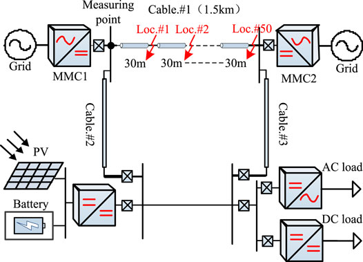
FIGURE 8. The structure of FDCDS.

Considering the limitations of simulation time-step and resolution for finding the fault location (Li et al., 2018), a frequency dependent $\pi$ cable model is adopted under small time-step simulation speed (50 $\mu \text{s}$), which is a lumped $\pi$ model with frequency dependent resistance and inductance.

In Figure 8, Cable #1 is divided into 50 sections equally (each section is 30 m), and Loc. #1 to Loc. #50 denote the end point of each section, respectively. Segments between every two Loc. # are marked as Sec. #1 to Sec. #50. Because the minimum distance is 30 m in each section, the resolution for fault location using the proposed method is 30 m.

Sample Data

DC loads fluctuation has a pretty big impact on power flow of FDCDS, so five types of DC loads are set to simulate the fluctuation (the rated power of DC loads is S_N, the actual power is S_real, and k represents the proportion of actual power in rated power, i.e., k = S_real/S_N): k is 80, 90, 100, 105, 110%, respectively. In order to make the fault location more accurate and give full play to learning and generalization ability of CNN, it is necessary to traverse the faults in various cases. In the training process of CNN, the following factors that may affect the location results need to be traversed: fault distance, fault pole, transient resistance, DC loads fluctuation, and distributed capacitance are considered during the training process of CNN. The traversal table of sample parameters is shown in Table 1, it can be worked out that the total sample number is 9000.The sampling frequency is 20 kHz, and the fault data is the fundamental frequency period after the fault is taken, therefore, the number of sampling points is 400. To sum up, the sample set from the measured voltage is 9000 × 400, and the output set is a matrix with dimension of 9000 × 50 after CNN to produce the results of the fault location.

TABLE 1

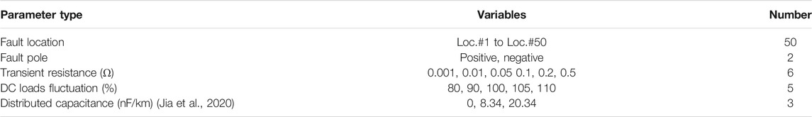
TABLE 1. The traversal table of sample parameters

Verification of the Proposed Method

Verification of Signal Analysis

The signal processing and CNN classification are all carried out on MATLAB 2020b. The PC used in the test platform with RAM of 12 GB has a CPU model of Inter (R) Core (TM) i7-10510U and a GPU model of NVIDIA GeForce MX250.

The correctness of the signal analysis is verified first. According to the signal processing procedure mentioned above, the voltage signals at 50 positions of Cable #1 in Figure 8 were extracted, respectively. After signal decomposition and transient energy calculation, the transient energy values of each signal decomposition frequency band as shown in Figure 9 were obtained. Most of the energy in the fault is concentrated in Level 1, 2, and 3, which is consistent with the previous analysis. Moreover, from the perspective of the transient energy of each frequency band from Loc. #1 to Loc. #50, the transient energy trend of Level 1, 2, and 3 are obvious and regular. Compared with other frequency bands, it is easier to form a mapping relationship between fault features and fault positions to complete high precision fault location.

FIGURE 9

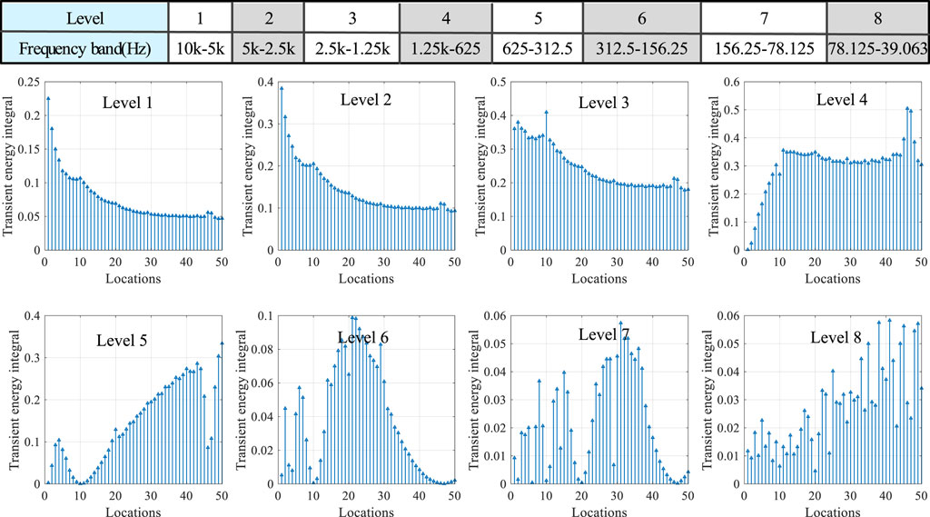
FIGURE 9. The transient energy of each signal decomposition level from Loc.#1 to Loc.#50.

Verification of CNN Classification

The structure, convolution kernel, and way of sub-sampling of CNN will have a big impact on the learning effect. In order to get the best parameters of CNN, many CNNs with different structure, convolution kernel, way of sub-sampling, and batch size are tested in this paper, and the most appropriate CNN structure was selected by comparing the training speed and accuracy. Finally, a typical structure of CNN is picked out after numerous experiments, in which its topology structure is 8C-2S-16C-2 S. The sub-sampling layer adopts mean-pooling, and the kernel size of convolution is 7 and 9, respectively. The gradient calculation method is stochastic gradient descent with momentum.

Figure 10 shows the changing trend of training accuracy and learning rate with epochs. In the early stage of training, the learning rate is relatively high, which ensures the training speed and accuracy. In the middle and late part of learning, when the training model tends to be stable, the learning rate is also significantly reduced, which ensures the effectiveness of the training model. The training process tends to be stable roughly at 2000 epochs, which is consistent with the change of learning rate. Finally, the accuracy of the fault location model obtained by training can reach more than 99%, almost close to 100%.

FIGURE 10

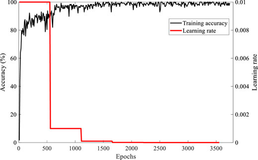
FIGURE 10. The curve changing of training accuracy and learning rate.

The output of softmax function is 50 values with a sum of one according to (1), and the category of the largest value is selected as the output result. Hence, when the fault occurs at the Loc. #1 to Loc. #50, the classification directly output the specific number of Loc. #, which is shown in Figure 11A. In addition, when there is a Sec. # fault, the output of the softmax function is two bigger values, which signifies that the fault is between these two locations, also known as Sec. # fault, just as shown in Figure 11B. Therefore, no matter which point on the line occurs the fault, the classifier will output the corresponding results (Loc. # fault or Sec. # fault).

FIGURE 11

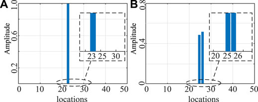
FIGURE 11. The location results. (A) Loc.# fault. (B) Sec.# fault.

To test the performance of trained CNN network in location accuracy, two fault types, Loc. # fault and Sec. # fault, with different transient resistances are tested, and the result is illustrated in Table 2. The fault positions on the line are random and do not always fall on the set fault points. Therefore, most of the fault points in the test fall randomly on the positions between the set fault points, i.e., Sec. # fault. Although the training data required in the process of model building is obtained by setting Loc. # fault, the test results show that the CNN model trained has a very high accuracy for Sec. # fault, which demonstrates the feasibility of softmax classifier in solving the fault location. When the location precision reaches 30 m, the final positioning can be carried out through manual inspection or UAV. Compared with the traditional line inspection method, the proposed method greatly reduces the time of fault location and improves the accuracy.

TABLE 2

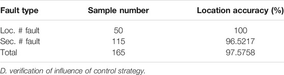
TABLE 2. The performance of the trained CNN

In the literature (Jia et al., 2020), the control strategy of MMC converter has an impact on the location accuracy, so the reliability of the proposed algorithm is tested by changing the control strategy of the MMC converter at both ends of Cable #1, when MMC1 is constant DC voltage control mode, MMC2 is constant power control mode and vice versa, and the test results are shown in Table 3.

TABLE 3

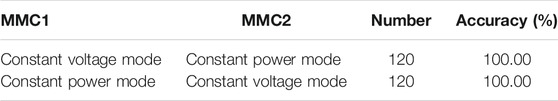
TABLE 3. Control strategy interference test results

As MMC adopts the modulation mode of step wave approaching the sinusoidal wave, the switching frequency of MMC is low, usually around 150 Hz. In the procedure of signal reconstruction, the frequency band range selected is from 1.25 to 10 kHz, which exceeds the switching frequency of the MMC converter. Therefore, the control strategy will not affect the location results. The input capacitor of the upper and lower bridge arm is unknown during the fault in the aforementioned analysis, which may cause the difficulty of the time-domain analysis. The frequency band range selected in this paper is 1.5–2 kHz, which belongs to the high frequency range. The SM’s capacitor impedance is -j/ωC₀, in which C₀ is the SM’s capacitor and ω = 2πf. In a high frequency domain, it is known that ωL_arm >> j/ωC₀. Therefore, the effect of the number of SM’s capacitor can be ignored at this stage.

Verification of the Fluctuation of PV’s Output Power

Most of the existing fault location methods in the flexible DC distribution network have poor application effects in practical projects, the main reason is that the location results are easily influenced by fluctuation of PV’s output power. In addition, the robustness of the proposed method is tested with the actual PV output power in a day. The output power of PV is mainly affected by illumination intensity. According to Equation (7), the per-unit value of PV’s output power in a day (assuming the maximum output power as the rated value) is calculated on the basis of the change of illumination intensity in a day. The accuracy of locating results is shown in Figure 12.

$P_{PV}=\{\begin{array}{cc}{P}_{pv}^r\frac{I}{I_r}& I\le I_r\\ P_{PV}^r& I>I_r\end{array}(7)$

where I is illumination intensity and Ir is rated intensity; and P_PV^r represents the rated value of PV’s output power and P_PV is the true output power of PV.

FIGURE 12

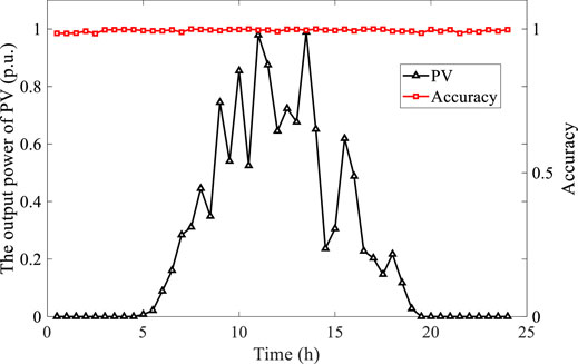
FIGURE 12. The influence of PV’s output power fluctuation on location accuracy.

The major influence of PV’s output fluctuation on the FDCDS is the change of power flow distribution in the system, so the changes of transient quantity in the fault are mainly concentrated in the low frequency band. In this paper, the frequency bands are selected by comparing the transient energy of each decomposition level, and the low frequency bands are filtered out because they contain only a small amount of feature information, already analyzed in the section on Fault Location Method. Therefore, PV’s output fluctuation has almost no effect on the accuracy of location, as shown in Figure 12. Furthermore, FDCDS has many branches connected to various types of loads and DGs, affecting the magnitude and distribution of the fault component. The boundary conditions of FDCDS at the line exit, composed of DC reactor and parallel filter, absorb and block the high frequency components of voltage and current, resulting in high frequency component of branches entered into the studied line being greatly reduced (Karmacharya and Gokaraju, 2018). Because the data used in the paper is the high frequency band of voltage, the influence of branches on positioning can be ignored. So, the fault location method proposed has a high robustness in the situation of massive branches access and is more valuable to the engineering application.

Comparisons With Existing Method

There are a lot of intelligent algorithms being applied to fault location of FDCDS, but few methods have solved the problems of long distribution lines and short resolution for located distance. In this paper, the resolution is set at 30 m, and the accurate location of 50 faults distances is realized. To verify the superiority of method in this paper, methods in literatures (Ye et al., 2020), (Chen et al., 2017), (Li et al., 2018), (Guifeng et al., 2014) are introduced to tested in FDCDS presented in article. Table 4. illustrates the comparing result of different methods when the noise’s SNR is 45dB. The evaluation criterions involve calculation time and iterations in the training phase, mean absolute error (MAE), root mean squared error (RMSE), and accuracy in the testing phase. The equation of MAE, RMSE, and accuracy is in (Equations 8–10):

$MAE=\frac{1}{N}{\displaystyle \sum _i^N\left|y_i-{\widehat{y}}_i\right|}(8)$

$RMSE=\sqrt{\frac{1}{N}{\displaystyle \sum _i^N{\left(y_i-{\widehat{y}}_i\right)}^2}}(9)$

$accuracy=\frac{n}{N}\times 100\%(10)$

here, N is the number of testing samples, y_i is the output value, ${\widehat{y}}_i$ is the true value, and n represents the number of samples whose output value is consistent with the true value in the testing process.

TABLE 4

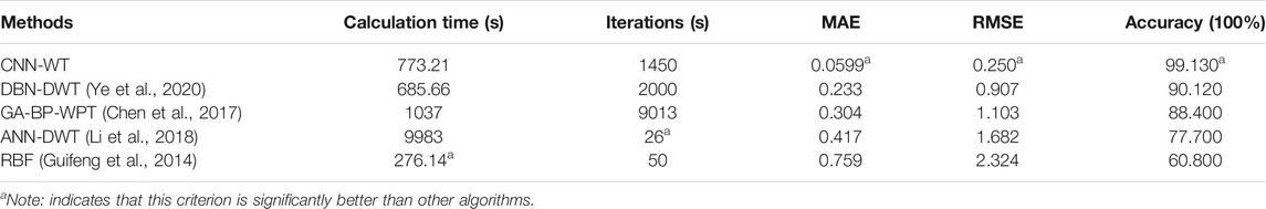
TABLE 4. Comparisons result of different methods when the SNR is 45 DB

The literature (Ye et al., 2020) develops a single pole-to-ground fault location method using wavelet decomposition and deep belief network (DBN), in which the low-frequency components and high-frequency components after three levels wavelet decomposition are used to characterize the fault’s overall trend. Although DBN with a stack of multiple RBMs is a strong classification, the feature extraction in frequency-domain is not sufficient to form a strong mapping relationship between fault distance and signal, so its performance is inferior to the proposed method in this paper.

Back-propagation (BP) optimized by genetic algorithm (GA) presented in the literature (Chen et al., 2017) utilizes wavelet packet decomposition to gather the signal energy of each frequency band and construct an energy feature vector. The test results show that the more detailed fault feature extracted, the more accurate the fault location. Aimed at ungrounded photovoltaic system, the literature (Li et al., 2018) proposes a location method that the high-frequency signal of fault information is extracted by DWT, and then the norm of different frequency bands’ detail coefficients is used as the input data vector for artificial neural network (ANN). Though this method ranging accuracy is accurate enough, the required sample frequency is quite high, which is up to 340 kHz. Therefore, at the sample frequency of 20 kHz, the method is difficult to identify 50 fault locations. To reflect the availability of signal analysis, the literature (Guifeng et al., 2014), which directly applies the radial basis function (RBF) neural network to use fault information to find fault distance, is regarded as a comparison to other smart algorithms with signal processing. The results in Table 4 show that the location method via RBF has the worst performance compared to the others though the training time is the shortest, so the signal analysis is necessary to extract fault characteristics when the location resolution is short, and the distribution line is quite long in FDCDS. It should be noted that the structures in the four classification methods are all optimized models based on the methods in the original literature under the environment created in this paper after vast tests, to guarantee the fairness and reliability of comparisons. From the comparison results, the MAE, RMSE, and accuracy criterions of the proposed method are significantly better than those of other methods under the same conditions.

In signal analysis and fault location, noise will affect the result, and Gaussian white noise following normal distribution is an important factor affecting fault location in the power system because of its strong randomness. In order to test the anti-interference ability of different methods aforementioned to noise, 9 groups of different signal-to-noise ratios (SNRs) from 5 dB to 45 dB are set for testing, and the SNRs reflect the ratio between normal signal and noise, which means that the higher the SNR, the closer the signal is to the normal signal.

Figure 13 gives the classification accuracy of different methods under different SNRs. When the signal interference is not large (more than 25dB), CNN with WT can have a better performance than other methods. Furthermore, when the SNRs are less than 20dB, the signal collected at this time contains a lot of interference, the proposed method still be much more accurate. But when the SNR comes to 5dB, the signal is already so distorted that any algorithms will lose accuracy. Due to the effective feature extracted in the signal processing and the elimination of noise interference, the proposed algorithm can achieve high precision fault location under noise interference comparing to four other methods.

FIGURE 13

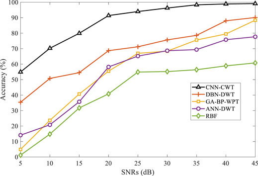
FIGURE 13. The classification accuracy of different methods under different SNRs.

Conclusion

In this paper, a fault location method with high precision is presented. DWT-based MRA is applied to decompose the voltage signal into 8 levels, and the signal bands with a large proportion of transient energy are selected for reconstruction. Then CWT is used to produce the grayscale images, which serve as the input of the CNN with the optimal structure and parameters under various tests after image enhancement.

A large number of simulation data show that the proposed method based on WT and CNN has a remarkable effect in the fault location of FDCDS, and eliminates the influence of the converter control strategy and the switching of SMs. Due to the effectiveness of the signal feature extraction, the method proposed in this paper still has high accuracy in the case of large-scale access of DGs with output fluctuation. Verification results of comparisons show that the proposed method has better performance and is more accurate and efficient than four other methods under various noises, thus it can be extended to complex FDCDS with little measuring points, which is of great significance to development of the DC system.

Data Availability Statement

The raw data supporting the conclusions of this article will be made available by the authors, without undue reservation.

Author Contributions

Idea and innovation of the paper: DW and BW; data collection: DW, WZ, and CZ; article writing: DW; revision of the paper: DW and JY.

Funding

This work was supported by the National Natural Science Foundation of China under Grant 51807092.

Conflict of Interest

The authors declare that the research was conducted in the absence of any commercial or financial relationships that could be construed as a potential conflict of interest.

Publisher’s Note

All claims expressed in this article are solely those of the authors and do not necessarily represent those of their affiliated organizations, or those of the publisher, the editors, and the reviewers. Any product that may be evaluated in this article, or claim that may be made by its manufacturer, is not guaranteed or endorsed by the publisher.

References

Chen, Y., Zhang, C., Zhang, Q., and Hu, X. (2017). “UAV Fault Detection Based on GA-BP Neural Network,” in Proceedings of 32nd Youth Academic Annual Conference of Chinese Association of Automation (YAC) (Hefei, China, 806–811. doi:10.1109/yac.2017.7967520

CrossRef Full Text | Google Scholar

Christopher, E., Sumner, M., Thomas, D., and de Wildt, F. (2011). “Fault Location for a DC Zonal Electrical Distribution Systems Using Active Impedance Estimation,” in Proceedings of 2011 IEEE Electric Ship Technologies Symposium (Alexandria, VA, USA, 310–314. doi:10.1109/ests.2011.5770888

CrossRef Full Text | Google Scholar

Dhar, S., Patnaik, R. K., and Dash, P. K. (2018). Fault Detection and Location of Photovoltaic Based DC Microgrid Using Differential Protection Strategy. IEEE Trans. Smart Grid 9 (5), 4303–4312. doi:10.1109/tsg.2017.2654267

CrossRef Full Text | Google Scholar

Gou, B., and Owusu, K. O. (2008). Linear Relation between Fault Location and the Damping Coefficient in Faulted Signals. IEEE Trans. Power Deliv. 23 (4), 2626–2627. doi:10.1109/tpwrd.2008.2002992

CrossRef Full Text | Google Scholar

Gu, J., Wang, Z., Ma, L., Kuen, J., Shahroudy, A., Shuai, B., et al. (2015). Recent Advances in Convolutional Neural Networks, Pattern Recognition, 77, 354–377. doi:10.1016/j.patcog.2017.10.013

CrossRef Full Text | Google Scholar

Guifeng, W., Hong, C., and Xuan, W. (2014). “Research of Small Current Grounding Fault Location Algorithm in Distribution Grid Based on RBF,” in Proceedings of 2014 International Conference on Information Science, Electronics and Electrical Engineering, 154–158. doi:10.1109/infoseee.2014.6948087Sapporo, Jpn. Nov.

CrossRef Full Text | Google Scholar

Guomin, L., Yingjie, T., Changyuan, Y., Yinglin, L., and Jinghan, H. (2018). Deep Learning‐based Fault Location of DC Distribution Networks. J. Eng. 2019, 3301–3305. doi:10.1049/joe.2018.8902

CrossRef Full Text | Google Scholar

Hao, Y., Wang, Q., Li, Y., and Song, W. (2018). An Intelligent Algorithm for Fault Location on VSC-HVDC System. Int. J. Electr. Power Energ. Syst. 94, 116–123. doi:10.1016/j.ijepes.2017.06.030

CrossRef Full Text | Google Scholar

He, Z.-y., Liao, K., Li, X.-p., Lin, S., Yang, J.-w., and Mai, R.-k. (2014). Natural Frequency-Based Line Fault Location in HVDC Lines. IEEE Trans. Power Deliv. 29 (2), 851–859. doi:10.1109/tpwrd.2013.2269769

CrossRef Full Text | Google Scholar

Huang, A. Q., Crow, M. L., Heydt, G. T., Zheng, J. P., and Dale, S. J. (2011). The Future Renewable Electric Energy Delivery and Management (FREEDM) System: The Energy Internet. Proc. IEEE 99 (1), 133–148. doi:10.1109/jproc.2010.2081330

CrossRef Full Text | Google Scholar

Huisheng Wang, Huisheng., and Keerthipala, W. W. L. (1998). Fuzzy-neuro Approach to Fault Classification for Transmission Line protection. IEEE Trans. Power Deliv. 13 (4), 1093–1104. doi:10.1109/61.714467

CrossRef Full Text | Google Scholar

Jia, K., Feng, T., Zhao, Q., Wang, C., and Bi, T. (2020). High Frequency Transient Sparse Measurement-Based Fault Location for Complex DC Distribution Networks. IEEE Trans. Smart Grid 11 (1), 312–322. doi:10.1109/tsg.2019.2921301

CrossRef Full Text | Google Scholar

Karmacharya, I. M., and Gokaraju, R. (2018). Fault Location in Ungrounded Photovoltaic System Using Wavelets and ANN. IEEE Trans. Power Deliv. 33 (2), 549–559. doi:10.1109/tpwrd.2017.2721903

CrossRef Full Text | Google Scholar

Kim, P. (2017). Training of Multi-Layer Neural Network, MATLAB Deep Learning : With Machine Learning, Neural Network and Artificial Intelligence. New York: Apress Media, 48–53. doi:10.1007/978-1-4842-2845-6_3

CrossRef Full Text | Google Scholar

Lee, H-J., Park, D-Y., Ahn, B-S., Deung-Yong Park, Y-M., Park, J-K., Bok-Shin Ahn, S. S., et al. (2000). A Fuzzy Expert System for the Integrated Fault Diagnosis. IEEE Trans. Power Deliv. 15 (2), 833–838. doi:10.1109/61.853027

CrossRef Full Text | Google Scholar

Li, J., Yang, Q., Mu, H., Le Blond, S., and He, H. (2018). A New Fault Detection and Fault Location Method for Multi-Terminal High Voltage Direct Current of Offshore Wind Farm. Appl. Energ. 220, 13–20. doi:10.1016/j.apenergy.2018.03.044

CrossRef Full Text | Google Scholar

Li, J., Li, Y., Xiong, L., Jia, K., and Song, G. (2020). DC Fault Analysis and Transient Average Current Based Fault Detection for Radial MTDC System. IEEE Trans. Power Deliv. 35 (3), 1310–1320. doi:10.1109/tpwrd.2019.2941054

CrossRef Full Text | Google Scholar

Li, Y., Zhang, S., Li, H., Zhai, Y., Zhang, W., and Nie, Y. (2012). A Fault Location Method Based on Genetic Algorithm for High-Voltage Direct Current Transmission Line. Euro. Trans. Electr. Power 22 (6), 866–878. doi:10.1002/etep.1659

CrossRef Full Text | Google Scholar

Liang, J., Jing, T., Niu, H., and Wang, J. (2020). Two-Terminal Fault Location Method of Distribution Network Based on Adaptive Convolution Neural Network. IEEE Access 8, 54035–54043. doi:10.1109/access.2020.2980573

CrossRef Full Text | Google Scholar

Lin, Q., Luo, G., and He, J. (20172017). Travelling‐wave‐based Method for Fault Location in Multi‐terminal DC Networks. J. Eng. 2017 (13), 2314–2318. doi:10.1049/joe.2017.0744

CrossRef Full Text | Google Scholar

Liu, H., Deng, Z., Li, X., Guo, L., Huang, D., Fu, S., et al. (2020). Oct.) the Averaged-Value Model of Flexible Power Electronics Substation in Hybrid AC/DC Distribution Systems. [Online]. Available: https://ieeexplore.ieee.org/document/9215150.

Google Scholar

Mallat, S. G. (1989). A Theory for Multiresolution Signal Decomposition: the Wavelet Representation. IEEE Trans. Pattern Anal. Machine Intelligence 11 (7), 674–693. doi:10.1109/34.192463

CrossRef Full Text | Google Scholar

Mohanty, R., Balaji, U. S. M., and Pradhan, A. K. (2016). “An Accurate Non-iterative Fault Location Technique for Low Voltage DC Microgrid,” “ in Proceedings of 2016 IEEE Power and Energy Society General Meeting (PESGM) (Boston, MA, USA, 1. doi:10.1109/pesgm.2016.7741136

CrossRef Full Text | Google Scholar

Mohsenian-Rad, H., and Davoudi, A. (2014). Towards Building an Optimal Demand Response Framework for DC Distribution Networks. IEEE Trans. Smart Grid 5 (5), 2626–2634. doi:10.1109/tsg.2014.2308514

CrossRef Full Text | Google Scholar

Tang, L., Dong, X., Shi, S., and Qiu, Y. (2019). A High-Speed protection Scheme for the DC Transmission Line of a MMC-HVDC Grid. Electric Power Syst. Res. 168, 81–91. doi:10.1016/j.epsr.2018.11.008

CrossRef Full Text | Google Scholar

Tawfik, M. M., and Morcos, M. M. (2005). On the Use of Prony Method to Locate Faults in Loop Systems by Utilizing Modal Parameters of Fault Current. IEEE Trans. Power Deliv. 20 (1), 532–534. doi:10.1109/tpwrd.2004.839739

CrossRef Full Text | Google Scholar

Wang, C., Jia, K., Bi, T., Xuan, Z., and Zhu, R. (2019). Transient Current Curvature Based protection for Multi‐terminal Flexible DC Distribution Systems. IET Generation, Transm. Distribution 13 (15), 3484–3492. doi:10.1049/iet-gtd.2018.5152

CrossRef Full Text | Google Scholar

Yan, X., CShu, C., and Yanjing, X. (2020). “Fault Location Method for DC Distribution Network Based on Impedance Parameters Identification,” in Proceedings of 2020 IEEE 3rd International Conference on Electronics Technology (ICET) (Chengdu, China, 378–381. doi:10.1109/icet49382.2020.9119551

CrossRef Full Text | Google Scholar

Ye, X., Lan, S., Xiao, S-J., and Yuan, Y. (2020). Single Pole-to-Ground Fault Location Method for MMC-HVDC System Using Wavelet Decomposition and DBN. IEEJ Trans. Electr. Electron. Eng. 16 (2), 238–247. doi:10.1002/tee.23290

CrossRef Full Text | Google Scholar

Yuan, Y., Kang, X., and Li, X. (2020). “A Fault Location Algorithm for DC Distribution Network Based on Transient Fault Components,” in Proceedings of 2020 5th Asia Conference on Power and Electrical Engineering (ACPEE) (Chengdu, China, 1316–1320. doi:10.1109/acpee48638.2020.9136507

CrossRef Full Text | Google Scholar

Zhao, S., Liu, Y., Han, Y., Hong, R., Hu, Q., and Tian, Q. (2018). Pooling the Convolutional Layers in Deep ConvNets for Video Action Recognition. IEEE Trans. Circuits Syst. Video Tech. 28 (8), 1839–1849. doi:10.1109/tcsvt.2017.2682196

CrossRef Full Text | Google Scholar

Zheng, X., Nadeem, M. H., Tai, N., Habib, S., Wang, B., Yu, M., et al. (2021). A Transient Current protection and Fault Location Scheme for MMC-HVDC Transmission Network. Int. J. Electr. Power Energ. Syst. 124, 1–9. doi:10.1016/j.ijepes.2020.106348

CrossRef Full Text | Google Scholar