 Helin Gong
 Zhang Chen
- Science and Technology on Reactor System Design Technology Laboratory, Nuclear Power Institute of China, Chengdu, China
The generalized empirical interpolation method (GEIM) can be used to estimate the physical field by combining observation data acquired from the physical system itself and a reduced model of the underlying physical system. In presence of observation noise, the estimation error of the GEIM is blurred even diverged. We propose to address this issue by imposing a smooth constraint, namely, to constrain the H1 semi-norm of the reconstructed field of the reduced model. The efficiency of the approach, which we will call the H1 regularization GEIM (R-GEIM), is illustrated by numerical experiments of a typical IAEA benchmark problem in nuclear reactor physics. A theoretical analysis of the proposed R-GEIM will be presented in future works.
1 Introduction and Preliminaries
In nuclear reactor simulations, data assimilation (DA) with reduced basis (RB) enables the reconstruction of the physical field, e.g., for constructing a fast/thermal flux and power field within a nuclear core in an optimal way based on neutronic transport/diffusion model and observations (Gong et al., 2016; Argaud et al., 2017a; Gong et al., 2017; Argaud et al., 2018; Gong, 2018). In practice, the existing methods are based on a reduced basis, however, this approach is not robust with respect to observation noise and there are some additional constraints or regularization on the low-dimensional subspaces, i.e., the related coefficients, have been proposed as possible remedies in several recent works (Argaud et al., 2017b; Gong et al., 2020; Gong et al., 2021). The idea of introducing box constraints was originally introduced in Argaud et al. (2017a) to stabilize the generalized empirical interpolation method in the presence of noise (Maday and Mula, 2013). The same idea has been applied to the POD basis and the background space (Gong et al., 2019) of the so-called parametrized-background data-weak (PBDW) data assimilation (Maday et al., 2015a). Recently, the regularization of the GEIM/POD coefficients has been studied in Gong et al. (2021). The corresponding theoretical analysis can be found in Gong (2018), Herzet et al. (2018), and Gong et al. (2019). This article introduces H1 regularization schemes for the approximation, and numerical experiments in nuclear reactor physics indicate its potential to address this obstruction.
Our goal is to approximate the physical state u from a given compact set
The algorithms used to build the reduced subspace
For reading convenience, let us first introduce some notations used throughout this article. We first introduces the standard L2(Ω) or
Let us denote by u (r; μ) the solution of a parameter-dependent partial differential equation (PDE) set on Ω and on a closed parametric domain
2 Field Reconstruction With Regularization
Our goal in this work is to infer any state
where
2.1 H1 Regularization
The goal of regularization is to prevent overfitting or to denoise in mathematics and particularly in the fields of inverse problems (Ivanov, 1976; Andreui et al., 1977; Balas, 1995; Arnold, 1998; Vladimir, 2012; Benning and Burger, 2018), by introducing additional information in order to solve ill-posed problems. From a Bayesian (James Press, 1989) point of view, regularization techniques correspond to introduce some prior distributions on model parameters. The general choice of R (u) is a norm-like form
If one would like to impose a smooth control, the H1 semi-norm can be used:
Examples can be found in the context of parameter estimation problems (Keung and Zou, 1998; Cai et al., 2008; Wilson et al., 2009; Barker et al., 2016), image-deblurring (Chan et al., 1997; Li et al., 2010; Cimrák and Melicher, 2012), image reconstruction (Ng et al., 2000), and flow control (Heinkenschloss, 1998; Collis et al., 2001). The work in Van Den Doel et al. (2012) shows that the proposed H1 semi-norm regularization performs better than L1 regularization cousin, total variation, for problems with very noisy data due to the smooth nature of controlled variables. The authors in Srikant did a comparison of H1 and TV regularization methods and also studied the shortcomings and limitations of some of the implementations schemes, such as a Gaussian filter. H1 regularization would perform well over uniform regions in the domain but would perform poorly over edges. Furthermore, to solve the PDE-constrained optimization problem as reported in Haber and Hanson (2007), the authors suggested a synthetic regularization functional of the form:
where the parameter γ can be adapted. Note that this synthetic regularization is now commonly used to solve the ill-posed inverse problems.
2.2 Generalized Empirical Interpolation Method
Recall that our goal is to estimate the state
The first step is to choose a sequence of n-dimensional subspaces
for an acceptable tolerance
In other words, we choose the subspaces such that the most dominant physical system is well represented for a relatively small n. In particular, these subspaces may be constructed through the application of model reduction methods to a parameterized PDE.
The second step is to model the data acquisition procedure. Given a system in of a parameter
where
where
We assume that em is independent and identically distributed (IID), and with a density of pm on
By running the greedy algorithm of the so-called generalized empirical interpolation method [GEIM (Maday and Mula, 2013)], a set of basis
With noisy observations, GEIM is, however, not robust with respect to observation noise (Argaud et al., 2017b), and in that work, a so-called constrained stabilized GEIM (CS-GEIM) by using a constrained least squares approximation was proposed to address this obstruction, where numerical experiments indicate its potential.
3 H1 Regularization Formulation of GEIM
Now, we state the H1 regularization scheme for GEIM (R-GEIM). Given a reduced space
where
• The basis and measurements of the chosen scheme could be based on GEIM, POD, or any other approach.
• Later, we will show that l = 2 corresponds to the least squares method, and l = 1 corresponds to the least absolute deviations (LAD) (Bloomfield and Steiger, 1980). Compared to the traditional least squares method, the LAD is much robust and finds its applications in many areas.
• By using the H1 regularization for the reduced basis field reconstruction, the first assumption is that the field u is in H1 space; for the most regular physical problem, this condition is satisfied automatically, and the H1 regularization term is a kind of smooth control for the underlying field reconstruction problem.
If we have no prior information about noise, a commonly used way to formulize Eq. 3.1 is taking 2 norm for the loss function term, we have the following results:
R-GEIM: Given a reduced space
Let
the solution is
Proof Let
the solution to minimize J (α,y) is the α∗ that satisfies ∇J (α∗,y) = 0. Because,
and the solution is
Later, we will show this is also the algebraic formulation for Gaussian noise with covariance
Remark Let r(u) be the bias of the reduced model from the truth
• Uniform noise, when the noise term em is uniformly independent and identically distributed on ( − e0, e0), then the reconstruction problem is: find
If the noise bounds are different for different measurements, the constraint in Eq. 3.7 becomes
• Gaussian noise, when the noise em is Gaussian with the zero mean and covariance matrix
• Laplacian noise, when the noise em is Laplacian independent, identically distributed with density
We refer readers to Boyd and Vandenberghe (2004) for further theoretical analysis on this remark. Through this remark, the physical means of the term
4 Numerical Results and Analysis
In this section, we illustrate the performance of R-GEIM on a typical benchmark problem in nuclear reactor physics. The test example is adapted based on the classical 2D IAEA benchmark problem (Benchmark Problem Book, 1977; Gong et al., 2017); the geometry of the 2D core is shown in Figure 1. This problem represents the mid-plane z = 190 cm of the 3D IAEA benchmark problem, that is used by references (Theler et al., 2011). The reactor spacial domain is Ω = region (1, 2, 3, 4). The core and control regions are Ωcore = region (1, 2, 3) and Ωcontrol = region (3), respectively. We consider the value of
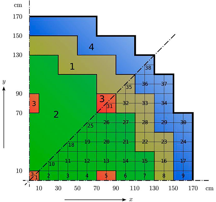
FIGURE 1. Geometry of a 2D IAEA benchmark. Upper octant: region assignments; lower octant: fuel assembly identification [from reference (Benchmark Problem Book, 1977; Theler et al., 2011)].
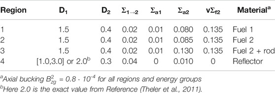
TABLE 1. Coefficient value: diffusion coefficients Di (in cm) and macroscopic cross sections (in cm-1).
The neutronic field (fast and thermal flux, power distribution) is derived by solving two group diffusion equations. The numerical algorithm is implemented by employing the free finite elements solver FreeFem++ (Hecht, 2012). The norm
The regularization factor ξ is essential for R-GEIM. It can significantly affect the reconstruction error of R-GEIM, and if they are incorrectly specified then the field reconstructed with R-GEIM is suboptimal. We show the variation of the errors in L∞, H1, and L2 norms for R-GEIM with respect to different regularization factors ξ in Figure 2. The dimension of reduced basis is fixed to n = 80, the number of measurements is set to m = 2n, and the observation noise is uniformly distributed, with a noise level σ = 10−2, 10−3. It can be observed that the optimal ξ is different for different error metrics. For the errors evaluated in L2 norm, the optimal ξop ∼ 0.1, and for L∞ norm or H1 norm, the optimal ξop ∼ 1. In the left of this work, we fix ξ to be the optimal value and evaluate the errors in L2 norm and H1 norm, which reflect the average error of the reconstructed field itself and its gradient.
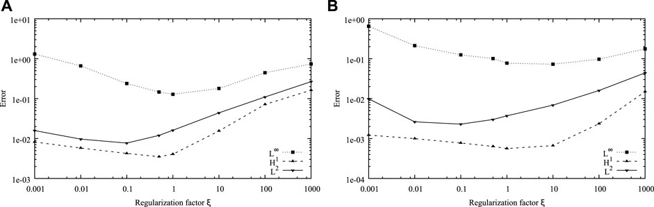
FIGURE 2. Variation of the errors in L∞, H1, and L2 norms for R-GEIM with respect to the different regularization factor ξ. The reduced dimension is n = 80, number of measurement is m = 2n, and the observation noise is uniformly distributed with noise levels 10−2 (A) and 10−3 (B).
This section illustrates the behavior of GEIM, CS-GEIM, and R-GEIM, in case of noisy observations. We first show the variation of the errors in L2 norm and H1 norm for GEIM, CS-GEIM, and R-GEIM with respect to different reduced dimensions n in Figure 3. The observation noise is assumed to be uniformly distributed, with a noise level σ = 10−2. The number of measurements is m = 2n. Figure 4 illustrates the case for the noise level σ = 10−3. The cases with Gaussian-distributed observation noise are shown in Figure 5 for the noise level σ = 10−2 and in Figure 6 for the noise level 10−3.
FIGURE 3. The variation of the errors in L2 norm (A) H1 norm (B) for GEIM, CS-GEIM, and R-GEIM with respect to different reduced dimension n. The number of measurement is m = 2n, and the observation noise is uniformly distributed with a noise level σ = 10−2.
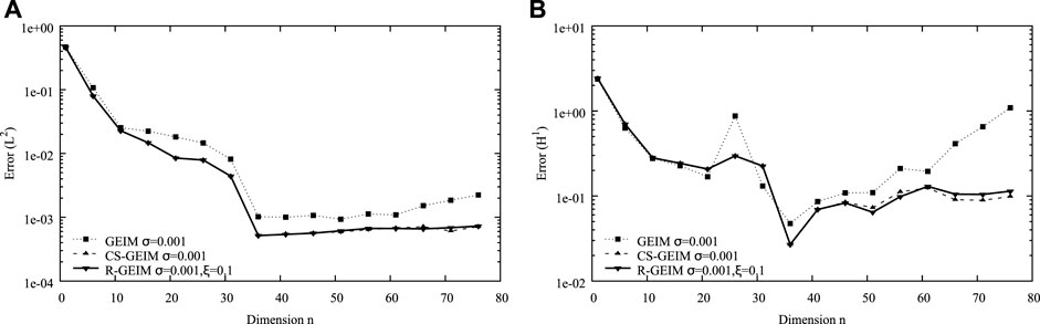
FIGURE 4. Variation of the errors in L2 norm (A) and H1 norm (B) for GEIM, CS-GEIM, and R-GEIM with respect to different reduced dimension n. The number of measurement is m = 2n, and the observation noise is uniformly distributed with a noise level σ = 10−3.
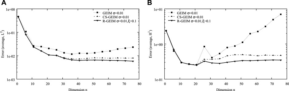
FIGURE 5. Variation of the errors in L2 norm (A) and H1 norm (B) for GEIM, CS-GEIM, and R-GEIM with respect to different reduced dimension n. The number of measurement is m = 2n, and the observation noise is Gaussian distributed with a noise level σ = 10−2.
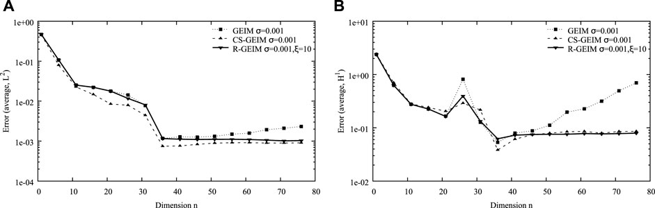
FIGURE 6. Variation of the errors in L2 norm (A) and H1 norm (B) for GEIM, CS-GEIM, and R-GEIM with respect to different reduced dimension n. The number of measurement is m = 2n, and the observation noise is Gaussian distributed with a noise level σ = 10−3.
From these figures, we can conclude that R-GEIM shows a better stability performance in the case of noisy measurement. The accuracy can be as good as CS-GEIM, but the R-GEIM algorithm is much simpler, with relatively low computational cost; the main cost for the online stage is to solve the matrix system Eq. 3.4. But for CS-GEIM, the relative complex constrained quadratic programming problem has to be solved.
5 Conclusion and Future Works
The traditional generalized empirical interpolation method is well studied for data assimilation in many domains. However, this reduced modeling-based data assimilation method is not robust with respect to observation noise. We propose addressing this issue by imposing a smooth constraint, namely, an H1 semi-norm of the reconstructed field to involve some prior knowledge of the noise. The efficiency of the approach, which we call R-GEIM, is illustrated by an IAEA benchmark numerical experiment, dealing with the reconstruction of the neutronic field derived from neutron diffusion equations in nuclear reactor physics. With H1 regularization, the behavior of the reconstruction is improved in the case of noisy observation. Further works are ongoing: i) mathematical analysis of the stable and accurate behavior of this regularization approach and ii) the regularization trade-off factor will be studied to give an outline on how to choose these factors for generic problems.
Data Availability Statement
The raw data supporting the conclusion of this article will be made available by the authors, without undue reservation.
Author Contributions
HG contributed to conceptualization, methodology, software, data curation, and writing—original draft and editing. ZC contributed to conceptualization. QL contributed to conceptualization, supervision, and review.
Funding
This work is supported by the National Natural Science Foundation of China (Grant No. 11905216 and Grant No. 12175220).
Conflict of Interest
The authors declare that the research was conducted in the absence of any commercial or financial relationships that could be construed as a potential conflict of interest.
Publisher’s Note
All claims expressed in this article are solely those of the authors and do not necessarily represent those of their affiliated organizations, or those of the publisher, the editors, and the reviewers. Any product that may be evaluated in this article, or claim that may be made by its manufacturer, is not guaranteed or endorsed by the publisher.
Acknowledgments
The authors are grateful to three reviewers for the useful remarks on the manuscript.
References
Andreui, N. T., Vasiliui, I. A., and Fritz, J. (1977). Solutions of Ill-Posed Problems, Volume 14. Washington, DC: Winston.
Argaud, J.-P., Bouriquet, B., Gong, H., Maday, Y., and Mula, O. (2017). “Stabilization of (G) EIM in Presence of Measurement Noise: Application to Nuclear Reactor Physics,” in Spectral and High Order Methods for Partial Differential Equations ICOSAHOM 2016 (Berlin, Germany: Springer), 133–145.
Argaud, J.-P., Bouriquet, B., de Caso, F., Gong, H., Maday, Y., and Mula, O. (2018). Sensor Placement in Nuclear Reactors Based on the Generalized Empirical Interpolation Method. J. Comput. Phys. 363, 354–370. doi:10.1016/j.jcp.2018.02.050
Argaud, J. P., Bouriquet, B., Gong, H., Maday, Y., and Mula, O. (2017). Stabilization of (G)EIM in Presence of Measurement Noise: Application to Nuclear Reactor Physics. Cham: Springer International Publishing, 133–145. doi:10.1007/978-3-319-65870-4_8
Arnold, N. (1998). Solving Ill-Conditioned and Singular Linear Systems: A Tutorial on Regularization. SIAM Rev. 40 (3), 636–666.
Balas, K. N. (1995). Sparse Approximate Solutions to Linear Systems. SIAM J. Comput. 24 (2), 227–234.
Barker, A. T., Rees, T., and Stoll, M. (2016). A Fast Solver for anH1Regularized PDE-Constrained Optimization Problem. Commun. Comput. Phys. 19 (1), 143–167. doi:10.4208/cicp.190914.080415a
Benchmark Problem Book (1977). Computational Benchmark Problem Comitee for the Mathematics and Computation Division of the American Nuclear Society. Argonne Code Center: Benchmark Problem Book.
Benning, M., and Burger, M. (2018). Modern Regularization Methods for Inverse Problems. Acta Numerica 27, 1–111. doi:10.1017/s0962492918000016
Bloomfield, P., and Steiger, W. (1980). Least Absolute Deviations Curve-Fitting. SIAM J. Sci. Stat. Comput. 1 (2), 290–301. doi:10.1137/0901019
Cai, X-C., Liu, S., and Zou, J. (2008). An Overlapping Domain Decomposition Method for Parameter Identification Problems. Domain Decomposition Methods Sci. Eng. XVII 2008, 451–458.
Chan, R. H., Chan, T. F., and Wan, W. L. (1997). Multigrid for Differential-Convolution Problems Arising from Image Processing. Proc. Workshop Scientific Comput. 1997, 58–72.
Chan, T. F., and Tai, X.-C. (2003). Identification of Discontinuous Coefficients in Elliptic Problems Using Total Variation Regularization. SIAM J. Sci. Comput. 25 (3), 881–904. doi:10.1137/s1064827599326020
Cimrák, I., and Melicher, V. (2012). Mixed Tikhonov Regularization in Banach Spaces Based on Domain Decomposition. Appl. Maths. Comput. 218 (23), 11583–11596.
Collis, S. S., Ghayour, K., Heinkenschloss, M., Ulbrich, M., and Ulbrich, S. (2001). Numerical Solution of Optimal Control Problems Governed by the Compressible Navier-Stokes Equations. Int. Ser. Numer. Math. 139, 43–55. doi:10.1007/978-3-0348-8148-7_4
De los Reyes, J-C., and Schönlieb, C-B. (2012). Image Denoising: Learning Noise Distribution via Pde-Constrained Optimization. arXiv preprint arXiv:1207.3425.
Gong, H., Argaud, J.-P., Bouriquet, B., and Maday., Y. (2016). “The Empirical Interpolation Method Applied to the Neutron Diffusion Equations with Parameter Dependence,” in Proceedings of PHYSOR.
Gong, H., Argaud, J. P., Bouriquet, B., Maday, Y., and Mula, O. (2017). “Monitoring Flux and Power in Nuclear Reactors with Data Assimilation and Reduced Models,” in International Conference on Mathematics and Computational Methods Applied to Nuclear Science and Engineering (M&C 2017), Jeju, Korea.
Gong, H. (2018). “Data Assimilation with Reduced Basis and Noisy Measurement: Applications to Nuclear Reactor Cores,” (Paris, France: Sorbonne University). PhD thesis.
Gong, H., Maday, Y., Mula, O., and Tommaso, T. (2019). Pbdw Method for State Estimation: Error Analysis for Noisy Data and Nonlinear Formulation. arXiv preprint arXiv:1906.00810.
Gong, H., Chen, Z., Maday, Y., and Li, Q. (2021). Optimal and Fast Field Reconstruction with Reduced Basis and Limited Observations: Application to Reactor Core Online Monitoring. Nucl. Eng. Des. 377, 111113. doi:10.1016/j.nucengdes.2021.111113
Gong, H., Yu, Y., and Li, Q. (2020). Reactor Power Distribution Detection and Estimation via a Stabilized Gappy Proper Orthogonal Decomposition Method. Nucl. Eng. Des. 370, 110833. doi:10.1016/j.nucengdes.2020.110833
Grepl, M. A., Maday, Y., Nguyen, N. C., and Patera, A. T. (2007). Efficient Reduced-Basis Treatment of Nonaffine and Nonlinear Partial Differential Equations. Esaim: M2an 41 (3), 575–605. doi:10.1051/m2an:2007031
Haber, E., and Hanson, L. (2007). Model Problems in PDE-Constrained Optimization. Report. Atlanta, GA, USA: Emory University.
Hecht, F. (2012). New Development in FreeFem++. J. Numer. Math. 20 (3-4), 251–265. doi:10.1515/jnum-2012-0013
Heinkenschloss, M. (1998). “Formulation and Analysis of a Sequential Quadratic Programming Method for the Optimal Dirichlet Boundary Control of Navier-Stokes Flow,” in Optimal Control, Theory, Algorithms, and Applications (Alphen aan den Rijn, Netherlands: Kluwer Academic Publishers BV). doi:10.1007/978-1-4757-6095-8_9
Herzet, C., Diallo, M., and Héas, P. (2018). An Instance Optimality Property for Approximation Problems with Multiple Approximation Subspaces. hal-01913339.
Ivanov, A. A. (1976). The Theory of Approximate Methods and Their Applications to the Numerical Solution of Singular Integral Equations, Volume 2. Berlin, Germany: Springer Science & Business Media.
James Press, S. (1989). Bayesian Statistics: Principles, Models, and Applications, Volume 210. Hoboken, NJ, USA: John Wiley & Sons.
Keung, Y. L., and Zou, J. (1998). Numerical Identifications of Parameters in Parabolic Systems. Inverse Probl. 14 (1), 83–100. doi:10.1088/0266-5611/14/1/009
Li, F., Shen, C., and Li, C. (2010). Multiphase Soft Segmentation with Total Variation and H 1 Regularization. J. Math. Imaging Vis. 37 (2), 98–111. doi:10.1007/s10851-010-0195-5
Maday, Y., and Mula, O. (2013). “A Generalized Empirical Interpolation Method: Application of Reduced Basis Techniques to Data Assimilation,” in Analysis and Numerics of Partial Differential Equations (Berlin, Germany: Springer), 221–235. doi:10.1007/978-88-470-2592-9_13
Maday, Y., Mula, O., and Turinici, G. (2016). Convergence Analysis of the Generalized Empirical Interpolation Method. SIAM J. Numer. Anal. 54 (3), 1713–1731. doi:10.1137/140978843
Maday, Y., Patera, A. T., Penn, J. D., and Yano, M. (2015). A Parameterized-Background Data-Weak Approach to Variational Data Assimilation: Formulation, Analysis, and Application to Acoustics. Int. J. Numer. Meth. Engng 102 (5), 933–965. doi:10.1002/nme.4747
Maday, Y., T, A., Penn, J. D., and Yano, M. (2015). PBDW State Estimation: Noisy Observations; Configuration-Adaptive Background Spaces; Physical Interpretations. Esaim: Proc. 50, 144–168. doi:10.1051/proc/201550008
Maday, Y., T, A., Penn, J. D., and Yano, M. (2015). Pbdw State Estimation: Noisy Observations; Configuration-Adaptive Background Spaces; Physical Interpretations. Esaim: Proc. 50, 144–168. doi:10.1051/proc/201550008
Ng, M. K., Chan, R. H., Chan, T. F., and Yip, A. M. (2000). Cosine Transform Preconditioners for High Resolution Image Reconstruction. Linear Algebra its Appl. 316 (1-3), 89–104. doi:10.1016/s0024-3795(99)00274-8
Rudin, L. I., Stanley, O., and Fatemi, E. (1992). Nonlinear Total Variation Based Noise Removal Algorithms. Physica D: Nonlinear Phenomena 60 (1-4), 259–268. doi:10.1016/0167-2789(92)90242-f
Theler, G., Bonetto, F. J., and Clausse, A. (2011). Solution of the 2D IAEA PWR Benchmark with the Neutronic Code Milonga. Actas de la Reunión Anual de la Asociación Argentina de Tecnología Nucl. XXXVIII.
Van Den Doel, K., Ascher, U., and Haber, E. (2012). The Lost Honour of L2-Based Regularization. Large Scale Inverse Problems, Radon Ser. Comput. Appl. Math. 13, 181–203.
Vladimir, A. M. (2012). Methods for Solving Incorrectly Posed Problems. Berlin, Germany: Springer Science & Business Media.
Wachsmuth, D., and Wachsmuth, G. (2011). “Necessary Conditions for Convergence Rates of Regularizations of Optimal Control Problems,” in System Modelling and Optimization (Berlin, Germany: Springer), 145–154.
Keywords: generalized empirical interpolation method, model order reduction, observations, regularization, nuclear reactor physics
Citation: Gong H, Chen Z and Li Q (2022) Generalized Empirical Interpolation Method With H1 Regularization: Application to Nuclear Reactor Physics. Front. Energy Res. 9:804018. doi: 10.3389/fenrg.2021.804018
Received: 28 October 2021; Accepted: 01 December 2021;
Published: 05 January 2022.
Edited by:
Qian Zhang, Harbin Engineering University, ChinaReviewed by:
Bertrand Bouriquet, Electricité de France, FranceZhang Chunyu, Sun Yat-Sen University, China
Jean-Philippe Argaud, Electricité de France, France
Copyright © 2022 Gong, Chen and Li. This is an open-access article distributed under the terms of the Creative Commons Attribution License (CC BY). The use, distribution or reproduction in other forums is permitted, provided the original author(s) and the copyright owner(s) are credited and that the original publication in this journal is cited, in accordance with accepted academic practice. No use, distribution or reproduction is permitted which does not comply with these terms.
*Correspondence: Helin Gong, Z29uZ2hlbGluMDZAcXEuY29t; Qing Li, bGlxaW5nX25waWNAMTYzLmNvbQ==