Two-Stage Energy Management for Energy Storage System by Using Stochastic Model Predictive Control Approach

There is a growing tendency for industrial consumers to invest in both photovoltaic (PV) and energy storage systems (ESSs) to meet their electricity requirements. However, the uncertainty of load demand and PV output brings great challenges for ESS operation. In this paper, a stochastic model predictive control (MPC) approach-based energy management strategy for ESSs is proposed. A non-parametric probabilistic prediction method embedded in time series correlation is adopted to describe the uncertainty of load demand and PV output. Then, a two-stage energy management model is proposed aiming at minimizing the total operation cost. The upper stage can generate an hourly operation strategy for ESSs, while the lower stage focuses on a more detailed minute-level operation strategy. The hourly operation strategy is also used as a basis to guide the ESS operation in the lower stage. Besides, a chance constraint was introduced to achieve a win–win solution between PV power consumption and electricity tariff, while the terminal value constraint of the capacity of ESSs to better cope with the uncertainty beyond the prediction time window. Finally, the numerical results showed that the proposed method can achieve an effective ESS energy management strategy.

Introduction

In recent years, photovoltaic (PV) panels and energy storage systems (ESSs) have been increasingly invested in to meet the requirements of developing renewable energy (Barchi et al., 2018; Liu et al., 2018, 2020). Distributed “PV+ESS” systems are helpful to energy consumption management and can reduce the operating costs of industrial companies. Moreover, distributed “PV+ESS” systems installed on the user side contribute to shaving the peak load, thereby delaying the expansion of distribution networks (Müller et al., 2018). However, the energy management of PV+ESS remain a challenging problem, especially on how to deal with uncertainty propagated by PV. Therefore, it is necessary to carry out energy management for PV+ESS to achieve maximal PV output consumption and reduce electricity costs.

In the energy management of PV+ESS, accurate PV output and consumer load demand predictions are of great importance (Nunna and Doolla, 2014; Sheikhi et al., 2015; Wang et al., 2017; Sharma et al., 2021). The probabilistic method is one of the most widely used approaches in the prediction of renewable generation output and demand (Wang et al., 2017; Wan et al., 2018; Huang et al., 2020). Studies (Nunna and Doolla, 2014; Sheikhi et al., 2015; Wang et al., 2017; Sharma et al., 2021) obtain the probability distributions of PV output and load demand from historical data and then employ the Monte Carlo method to generate a large number of scenarios to describe the uncertainty. The probabilistic methods can be divided into two main categories: parameterized (Reddy et al., 2015) and non-parametric probabilistic forecasting method (Zhou et al., 2019; Wan et al., 2020). Parameterized probabilistic forecasting method can explicitly express the functional relationship among the probability predictor variables. However, the accuracy of this type of method is strongly related to the accuracy of parameter calibration. The error of the prediction result may be large when the parameter accuracy is low. Among the non-parametric probabilistic forecasting methods, the quantile prediction method is currently the most popular (Dumas et al., 2021), which does not assume a specific distribution and can obtain more accurate and flexible forecast results of consumers’ energy consumption and PV output. Thus, it was adopted in this paper to make the prediction of PV output and demand.

Considering the future state of charge (SOC) is important for ESSs to make decisions, especially after being integrated with devices that introduce uncertainties (Tang et al., 2020, 2021; Li et al., 2021). The length of the prediction time window and the time granularity could respectively affect the prediction accuracy (Shangguan et al., 2021) and the corresponding computational burden. A longer prediction time window can cover the uncertainty for a longer period, but takes more time to solve. On the contrary, a shorter one takes less time to solve, but may be unable to avoid the problem caused by uncertainty (Małkowski et al., 2021). Therefore, it is necessary to choose a reasonable length of prediction time window and prediction granularity according to the demands of real-world applications.

Several existing works (Atzeni et al., 2013; Spiliopoulos et al., 2017; Xu et al., 2018; Bakeer et al., 2021) have made contributions to ESS management. Atzeni et al. (2013). proposed an optimal operation strategy for a smart grid in which users reduce their electricity expenses by managing owned energy storage devices. Spiliopoulos et al. (2017) focused on maximizing the economic benefits of users who had ESSs installed. Atzeni et al. (2013) and Spiliopoulos et al. (2017) explored the commercial value of ESSs to the user side and proposed their benefit functions. Compared with those of the day-ahead prediction of renewable energy output and load demand, the prediction data obtained during intraday operation were more accurate. Hence, Xu et al. (2018) chose to formulate an optimal intraday rolling operation model of energy storage with the prediction data during the intraday. Yin et al., (2018) adopted model predictive control (MPC) to realize the intraday rolling optimal scheduling of ESSs. However, the guidance of day-ahead schedules to the intraday operation was ignored in the above works. To this end, we leveraged the SOC schedules from the long-term operation scheduling to guide the short-term scheduling in the intraday operation, leading to a better consideration of the uncertainty beyond the prediction time window in the short-term operation model. Moreover, to better integrate renewable energy, chance constraints were introduced to restrict the integration risk, which can make a better trade-off between the economic benefit and integration capacity.

To sum up, focusing on minimizing electricity costs, this paper proposes a two-stage rolling energy management scheme that is driven by stochastic MPC. It combines time intervals with coarse and fine time granularity and can achieve precise optimal control of ESSs. Chance constraints were introduced to restrict the integrated capacity of renewable energy, and terminal SOC constraints were added to better deal with the uncertainty from the prediction time window. Probabilistic forecasting methods were used to describe the uncertainty of PV output and demand, providing data support to energy management. The effectiveness of the method proposed in this paper was verified through the analysis of numerical case studies. The main contributions of this paper are as follows:

1) A stochastic MPC-based energy management strategy for ESSs is proposed. It is helpful to energy consumption management and can reduce the operating costs of industrial companies.

2) A scenario generation method based on the non-parametric probabilistic prediction method embedded in time series correlation is adopted to describe the uncertainty of demand and PV output.

3) The terminal value constraint of the capacity of ESSs is introduced to cope with the uncertainty beyond the prediction time window. It can better cover the space requirements of energy storage in the near future.

This paper is organized as follows: Introduction presents the framework of the proposed model. The Framework of the Proposed Model gives the details of the probabilistic prediction-based scenario generation method. The energy management scheme based on stochastic MPC is detailed in Scenario Generation Method Based on the Probabilistic Prediction Method. Several cases are tested in The Energy Management Strategy Based on Stochastic MPC to validate the effectiveness of the proposed method. Conclusion summarizes this paper.

The Framework of the Proposed Model

ESSs may fail to endure charging or discharging for a long period due to the limited stored energy and storage capacity. Therefore, it is necessary to consider future energy requirements of ESSs when scheduling charging and discharging. The scheduling time horizon of the rolling optimization problem is designed to have two timescales. The coarse time granularity scheduling of ESSs is formulated based on an hourly timescale. The longer the forecast time window of the hourly timescale, the more adequate is the consideration of future requirements. The fine time granularity scheduling of ESSs is formulated based on a minute timescale, and its prediction time window is shorter compared with that of hourly scheduling. In the minute timescale, the step size of the control is usually set as 5–15 min to better adapt the power fluctuation, ensuring a good tracking effect of ESSs. In this paper, the step size of the control for the fine granularity scheduling is set as 5 min. The framework for the two-stage operation model is shown in Figure 1.

FIGURE 1

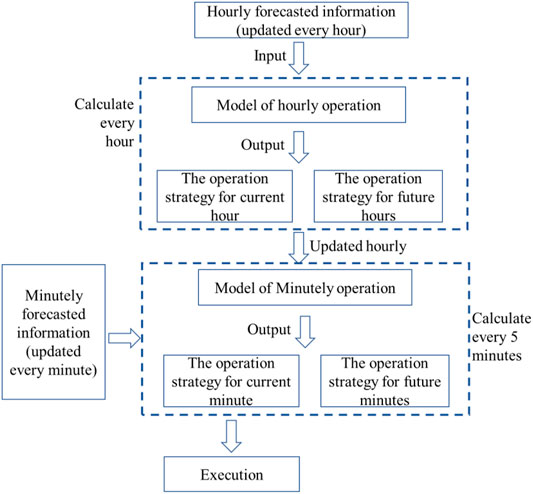
FIGURE 1. Flowchart of the two-stage operation model.

Both the hourly and the 5-min timescale operation models were based on the stochastic MPC approach. Thus, they share the same framework, which is shown in Figure 2, and include the following steps:

Step 1: Initialize or update information. The information includes the current SOC of the ESS, real-time demand and output of renewable generation, and the most recently updated load and renewable generation output forecasts. These pieces of information are used to conduct the control strategy.

Step 2: Calculate the optimal control strategy. The control strategy can be calculated by solving the finite-time control problem with the above-mentioned information.

Step 3: Execute the strategy. The control strategy for the binding time interval will be executed; then, go back to step 1.

FIGURE 2

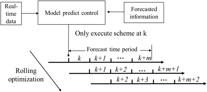
FIGURE 2. Illustration of model predictive control (MPC).

Scenario Generation Method Based on the Probabilistic Prediction Method

Compared with the deterministic prediction method, the probabilistic prediction method can provide more comprehensive prediction information and is more conducive to accurate prediction of user demand and PV output. Because the procedures to predict load and PV output are the same, we used the demand prediction as an example to introduce the prediction procedure.

Probability Distribution

The quantile regression is used to obtain the estimates of the quantiles of the load distribution. The specific quantile model of the load can be written as Eqs. 1 and 2.

$\mathrm{Pr}\left(D_t\le k_t^{\alpha }\right)=\alpha (1)$

$k_t^{\alpha }=F_t^{-1}\left(\alpha \right)(2)$

${\widehat{F}}_t=\left\{{\widehat{k}}_t^{{\alpha }_i}|0\le {\alpha }_1\le \dots \le {\alpha }_N\le 1\right\}(3)$

where $\mathrm{Pr}\left(\right)$ is the probability operator; $D_t$ is the load at time t; $\alpha$ represents the level of $k_t^{\alpha }$$k_t^{\alpha }$; and $F_t\left(\right)$ is the cumulative distribution function of the load; ${\widehat{F}}_t$ represents the predicted quantile sequence at time t spanning from 0 to 1, which is used to represent the cumulative distribution function curve of load forecasting. For each moment, there is a set of predicted quantile sequences. $k_t^{\alpha }$ is the actual quantile and ${\widehat{k}}_t^{{\alpha }_i}$ represents the estimated value. $N$ represents the number of quantiles.

There are four steps to obtain the probability distribution:

a) Obtain the quantile sequence via Eqs. 1–3.

b) Use the linear interpolation method to process the quantile sequence to obtain the cumulative distribution function curve $F_t\left(\right)$$F_t\left(\right)$.

c) Use the uniform sampling method to generate a set of random variables, $\mathit{y}={\left[y_1,y_2,\dots ,y_T\right]}^T$.

d) By solving the inverse function $D_t=F_t^{-1}\left(\alpha \right)$, the cumulative probability of the load $\mathit{D}=D_1,D_2,\dots ,D_T$ is obtained.

Scenario Generation Method Embedded Time Series Correlation

With the obtained probability distribution, a series of forecasted scenarios of the load can be generated by the random sampling method. These generated scenarios that retain the probability characteristics and time series correlation of the load can simulate the load change. On the basis of the probabilistic prediction model, the multivariate Gaussian Copula method can be used to define the correlation structure of the load and can realize the load prediction, which considers the time series correlation. This method comprises five steps to generate scenarios:

Step 1: Construct the multivariate cumulative distribution function. On the basis of the probability prediction model, the multivariate Gaussian Copula function is further introduced to construct a new multivariate cumulative distribution function, $F\left(D_1,D_2,\dots ,D_T\right)$, that fits the time series correlation of the load.

$F\left(D_1,D_2,\dots ,D_T\right)=C\left(F_1\left(D_1\right),F_2\left(D_2\right),\dots ,F_T\left(D_T\right)\right)=C\left(y_1,y_2,\dots ,y_T\right)(4)$

Step 2: Generate the quantile sequence. Generate uniformly distributed quantile sequences, $\mathit{a}=\left[a_1,a_2,\dots ,a_T\right]$, within [0,1].

Step 3: Obtain the value of the random variable $y_i$. Firstly, define $C\left(y_1,1,\dots ,1\right)=a$ to calculate the actual value $y_1^{\ast }$ of the first random variable $y_1$. Secondly, let the partial derivative of the second random variable $y_2$ be equal to $a_2$, which is the value of marginal cumulative distribution function.

${\frac{{\partial }^{T-1}C\left(y_1,y_2,1,\dots ,1\right)}{\partial y_1}|}_{y_1=y_1^{\ast }}=a_2(5)$

Then, the value of the second variable $y_2^{\ast }$ can be obtained via solving the partial derivative Eq. 5, and then let $y_2=y_2^{\ast }$. Thirdly, make the partial derivative of the third random variable $y_3$ equal to $a_3$ and obtain the value of the third random variable by solving the partial derivative Eq. 6. Finally, repeat these steps until the last one is solved.

${\frac{\frac{{\partial }^{T-1}C\left(y_1,y_2,y_3,1,\dots ,1\right)}{\partial y_1\partial y_2}}{\frac{{\partial }^{T-1}C\left(y_1,y_2,1,\dots ,1\right)}{\partial y_1\partial y_2}}|}_{y_1=y_1^{\ast },y_2=y_2^{\ast }}=a_3(6)$

Step 4: Generate a quantile series. Repeat steps 2 and 3 for M times. Let the result ${\left[y_1^{\ast },y_2^{\ast },\dots ,y_T^{\ast }\right]}^T$ obtained in the ith iteration be vector $y_i^{\ast }$. Finally, M sampling values $y_i^{\ast },i=\mathrm{1,2},\dots ,M$, for the multivariate random variable y, can be obtained.

Step 5: Generate load scenarios. With the quantile sequence obtained in step 4, the time-dependent load sequences ${\mathit{D}}_i^w={\left[D_{i,1},D_{i,2},\dots ,D_{i,T}\right]}^T$ can be calculated via the inverse function $D_{i,t}=F_t^{-1}\left(y_{i,t}^{\ast }\right)$.

A series of time-dependent load scenarios of users can be generated via the above method. The generated scenarios can be used to convert the uncertain problem into a deterministic problem. It should be noted that a large-scale scenario set will result in a problem that is difficult to solve. Hence, in this paper, the k-means clustering algorithm is adopted to reduce the scale of scenarios for reducing the solution time while retaining the uncertain feature of the load. The occurrence probabilities of the centric scenarios in the clusters will be different, but their sum will always be equal to 1.

The Energy Management Strategy Based on Stochastic MPC

The General Form

The general form of the stochastic MPC-based optimal operation model is formulated as follows. The objective value is written as Eq. 7. The state function is formulated as Eq. 8. Equations 9 and 10 are respectively the chance constraints of the status and inputs. Equation 11 represents the terminal value constraints.

${\min }_{{\left\{{\pi }_{k+1}\right\}}_{j=0}^{N-1}}{E}_{x_k}\left[{\displaystyle {\sum }_{j=0}^{N-1}J\left(x_{k+j},{\pi }_{k+j}\right)+J_N\left(x_{k+N}\right)}\right](7)$

$x_{k+1}=A{x}_k+B{u}_k+G{\omega }_k(8)$

$\mathrm{Pr}\left(E_x{u}_{k+j}\le 1\right)\ge 1-\epsilon ,j\in N_{\left[0,N-1\right]}(9)$

$\mathrm{Pr}\left(E_u{u}_{k+j}\le 1\right)\ge 1-\epsilon ,j\in N_{\left[0,N-1\right]}(10)$

$T_f\left(\right)\le 0(11)$

where ${\left\{{\pi }_{k+1}\right\}}_{j=0}^{N-1}$ is the control rate, $x_k$ represents the system state variables, $u_k$ is the system input, and ${\omega }_k$ represents the noise. The value of noise ${\omega }_k$ at time k and the future are unknown. N is the time window of the forecasting time period and $\epsilon$ is the probabilistic value of chance constraints. Overall, the stochastic MPC problem can be considered as a stochastic programming problem.

To apply the above general stochastic MPC model to the proposed two-stage energy management of ESSs, the following three aspects need to be figured out: 1) input variables, including the current load $D_t$, the current PV output $P_t^{\mathrm{Solar},\mathrm{Max}}$, and the electricity price $C_t$; 2) state variables, including the ESS SOC $E_t$, the ESS charging power $P_t^{\mathrm{chr}}$, the ESS discharging power $P_t^{\mathrm{dis}}$, and the matching score of the ESS to the day-ahead schedule $G_t$; 3) noise information, including the uncertainty of the predicted PV output $P_{t+\Delta t}^{\mathrm{Solar},\mathrm{Max}}$ and the load value $D_{t+\Delta t}$.

The Two-Stage Energy Management Model

In this paper, the proposed energy management scheme of ESSs includes two parts: the upper stage (coarse time granularity scheduling) and the lower stage (fine time granularity scheduling). The time interval of the upper stage (hourly operation) is indexed by $H=\left\{\mathrm{0,1,2},\dots ,23\right\}$; the time interval of the lower stage (hourly operation) is represented by $\tau =\left\{0,\Delta t,2\Delta t,\dots ,11\Delta t\right\}$. A complete operation cycle can be represented by multiplying two vectors, $\left(h,t\right)\in H\times \tau$, where $\left(h,11\Delta t+\Delta t\right)=\left(h+\mathrm{1,0}\right)$. It is worth noting that, at different timescales, the model framework remains unchanged.

The Upper Stage

The coarse time granularity scheduling in the upper stage focuses on providing a reference to the underneath fine time granularity scheduling. Particularly, in the upper stage, the forecast step of renewable generation output and load is set as hourly, and the forecast time window is set as the whole day. The objective function of the hourly operation scheduling can be written as Eq. 12, minimizing user electricity expense. In this stage, the subscript of the lower stage t is omitted.

$\min {\displaystyle {\sum }_{s=1}^{S_c}{\pi }_s}{\displaystyle {\sum }_{h=h_0}^{23}\left[C\left(E_{h,s},{\mathit{p}}_{h,s}^{\mathrm{Ess}}\right)|E_{\mathrm{0,0}}\right]+c^{cap}\cdot p^{\mathrm{Grid},\mathrm{Max}}}(12)$

$C\left(E_{h,s},{\mathit{p}}_{h,s}^{\mathrm{Ess}}\right)=c_h\left(p_{h,s}^{\mathrm{chr}}-p_{h,s}^{\mathrm{dis}}\right)\cdot \Delta h(13)$

where ${\pi }_s$ represents the probability of scenario s; $C\left(E_{h,s},{\mathit{p}}_{h,s}^{\mathrm{Ess}}\right)$ represents the operation cost for hourly operation; $E_{\mathrm{0,0}}$ represents the initial energy status of the ESS; and $c^{\mathrm{cap}}$ represents the capacity price for electricity supply. $p^{Grid,Max}$ represents the upper bound of power from the grid during the whole operation period. $c_h$ is the energy price at hour h.

Energy Evolution Function

The energy evolution function of the hourly energy management model is written as follows:

$E_{h+1,s}=E_{h,s}+p_{h,s}^{\mathrm{chr}}\cdot {\eta }^{\mathrm{chr}}{1}_{\left\{\left(p_{h,s}^{\mathrm{chr}}-p_{h,s}^{\mathrm{dis}}\right)<0\right\}}-p_{h,s}^{\mathrm{dis}}\cdot 1_{\left\{\left(p_{h,s}^{\mathrm{chr}}-p_{h,s}^{\mathrm{dis}}\right)<0\right\}}/{\eta }^{dis}(14)$

where ${\eta }^{\mathrm{chr}}$ and ${\eta }^{\mathrm{dis}}$ respectively represent the charging efficiency and discharging efficiency. $1_{\{\ast \}}$ is an indicator function, which returns 1 if the function in {} is true; otherwise, it returns 0.

State Variables

State variables include energy, $E_{h,s}$$E_{h,s}$; charging power, $p_{h,s}^{\mathrm{chr}}$; discharging power, $p_{h,s}^{\mathrm{dis}}$$p_{h,s}^{\mathrm{dis}}$; charging indicator, $y_{h,s}$; and discharging indicator, $z_{h,s}$. Constraints include four different sets, namely, power balance constraints as in Eq. 15, energy limits as in Eq. 16, and the charging and discharging power limits as in Eqs. 17 and 18. Constraint 19 forces the charging and discharging of ESSs to be exclusive.

$D_{h,s}+\left(p_{h,s}^{\mathrm{chr}}-p_{h,s}^{\mathrm{dis}}\right)=p_{h,s}^{\mathrm{Grid}}+p_{h,s}^{\mathrm{solar}}(15)$

$E^{min}\le E_{h,s}\le E^{\max }(16)$

$0\le p_{h,s}^{\mathrm{chr}}\le y_{h,s}\cdot p^{\mathrm{Ess},\max }(17)$

$0\le p_{h,s}^{\mathrm{dis}}\le z_{h,s}\cdot p^{\mathrm{Ess},max}(18)$

$y_{h,s}+z_{h,s}\le 1(19)$

In Eqs. 15–19, $p_{h,s}^{\mathrm{Grid}}$ represents the power obtained from the grid; $p_{h,s}^{\mathrm{solar}}$ is the dispatch of PV; and $E^{\max }$ and $E^{\min }$ are the upper and lower energy bounds of ESS, respectively. $y_{h,s}$ is the charging status and $z_{h,s}$ is the discharging status. $p_{h,s}^{\mathrm{solar}}$ is the forecast value of the PV output.

Input Variables

The load and PV output are defined as the input variables. In this paper, the proposed model needs to fully supply the load, and the load forecast will be updated as in Eq. 15. In addition, the PV output constraints are formulated as

$0\le p_{h,s}^{\mathrm{solar}}\le p_{h,s}^{\mathrm{solar},Max}(20)$

Chance Constraints

To better integrate PV, chance constraints were introduced. The widely used chance constraint for renewable energy integration is shown in Eq. 21. It represents that the actual use of PV power is higher than its predicted value by 90%, and the probability of PV power usage should be higher than $\beta$.

$\mathrm{Pr}\left(90\%\cdot p_{h,s}^{\mathrm{solar},Max}\le p_{h,s}^{\mathrm{solar}}\le p_{h,s}^{\mathrm{solar},Max}\right)\ge \beta (21)$

Tang et al. (2019) proposed an improved chance constraint model where the expected value of the integrated renewable energy output is higher than 90% of its predicted scenarios. The improved model can be formulated as

$E\left[{\displaystyle {\sum }_{s=1}^S{\displaystyle {\sum }_{h=1}^T{p}_{h,s}^{\mathrm{solar}}}}\right]\ge 90\%{\displaystyle {\sum }_{s=1}^S{\displaystyle {\sum }_{h=1}^T{p}_{h,s}^{\mathrm{solar},Max}}}(22)$

With the introduction of scenario weights, constraint 22 can be rewritten as Eq. 23. Compared with the original chance constraints, the modified model can be solved via a commercial solver, such as Cplex and Gurobi.

${\displaystyle {\sum }_{s=1}^S{\pi }_s}{\displaystyle {\sum }_{h=1}^T{p}_{h,s}^{\mathrm{solar}}}\ge 90\%E\left[{\displaystyle {\sum }_{s=1}^S{\pi }_s}{\displaystyle {\sum }_{h=1}^T{p}_{h,s}^{\mathrm{solar},Max}}\right](23)$

Terminal Energy Constraints

As an energy-limited device, we introduce the energy constraint of ESSs to force the terminal energy back to the initial value to ensure their effective periodic operation. This constraint can be written as:

$E_{H,s}=E_{0,s}(24)$

where $E_{0,s}$ and $E_{H,s}$ represent the initial and terminal energy, respectively.

The Lower Stage

The lower stage gives the details of the minute-level operation, which focuses on maintaining the power balance in a short period and is conducive to smoothing the output of integrated PV. The objective function of the minute-level energy management model is written as Eq. 25.

$\min {\displaystyle {\sum }_{s=1}^{S^{EB}}{\pi }_s}{\displaystyle {\sum }_{t=t_0}^{T^{\mathrm{EB}}}\left[C^{EB}\left(E_{t,s}^{\mathrm{EB}}{E}_{h,s},\Delta {\mathit{p}}_{t,s}^{\mathrm{Ess}}\right)|E_0^{\mathrm{EB}}\right]+c^{\mathrm{cap}}\cdot p^{Grid,Max}}(25)$

$C^{EB}\left(E_{t,s}^{\mathrm{EB}}{E}_{h,s},\Delta {\mathit{p}}_{t,s}^{\mathrm{Ess}}\right)=c_t\left(\Delta p_{h,s}^{\mathrm{chr}}-\Delta p_{h,s}^{\mathrm{dis}}\right)\cdot \Delta t(26)$

where $\Delta {\mathit{p}}_{t,s}^{\mathrm{Ess}}$ includes two parts, namely, the deviation of charging power $\Delta p_{h,s}^{\mathrm{chr}}$ and the discharge power $\Delta p_{h,s}^{\mathrm{dis}}$$\Delta p_{h,s}^{\mathrm{dis}}$. $S^{\mathrm{EB}}$ represents the scenario number of the minute-level operation; $T^{\mathrm{EB}}$ represents the time interval for the minute-level operation; $C^{EB}\left(E_{t,s}^{\mathrm{EB}}{E}_{h,s},\Delta {\mathit{p}}_{t,s}^{\mathrm{Ess}}\right)$ is the operation cost of the deviation operation of energy storage; $E_0^{\mathrm{EB}}$ is the initial operation status of energy storage for the minute-level operation; and $c_t$ represents the electricity price.

Energy Evaluation Function

The minute-level energy evaluation function is similar to that of the hour-level model and further considers the change in the charging and discharging power. Hence, this energy evaluation function can be written as:

$\begin{array}{l}{E}_{h,t+\Delta t,s}=E_{h,t,s}+p_{h,s}^{\mathrm{chr}}\cdot {\eta }^{\mathrm{chr}}{1}_{\left\{\left(p_{h,s}^{\mathrm{chr}}-p_{h,s}^{\mathrm{dis}}\right)<0\right\}}-p_{h,s}^{\mathrm{dis}}\cdot \frac{1_{\left\{\left(p_{h,s}^{\mathrm{chr}}-p_{h,s}^{\mathrm{dis}}\right)<0\right\}}}{{\eta }^{\mathrm{dis}}}\\ +\Delta p_{h,s}^{\mathrm{chr}}\cdot {\eta }^{\mathrm{chr}}{1}_{\left\{\left(p_{h,s}^{\mathrm{chr}}-p_{h,s}^{\mathrm{dis}}\right)<0\right\}}-\Delta p_{h,s}^{\mathrm{dis}}\cdot \frac{1_{\left\{\left(p_{h,s}^{\mathrm{chr}}-p_{h,s}^{\mathrm{dis}}\right)<0\right\}}}{{\eta }^{\mathrm{dis}}}\end{array}(27)$

State Constraints

Similarly, the state constraints of the minute-level operation model are also made up of four different parts: 1) the power balance in Eq. 28; b) the capacity constraints of energy storage in Eq. 29; c) the charging and discharging power constraints of energy storage shown Eqs. 30 and 31; and d) the status constraints of energy storage in Eq. 32. Based on the state constraints of the hour-level operation model, all the following formulations further consider adjusting the charging and discharging power of the energy storage during the minute-level operation period.

$D_{h,t,s}+\left(p_{h,t,s}^{\mathrm{chr}}-p_{h,t,s}^{\mathrm{dis}}\right)+\left(\Delta p_{h,t,s}^{\mathrm{chr}}-\Delta p_{h,t,s}^{\mathrm{dis}}\right)=p_{h,t,s}^{\mathrm{Grid}}+p_{h,t,s}^{\mathrm{solar}}(28)$

$E^{\min }\le E_{h,t,s}\le E^{\max }(29)$

$0\le p_{h,t,s}^{\mathrm{chr}}+\Delta p_{h,t,s}^{\mathrm{chr}}\le y_{h,t,s}\cdot p^{\mathrm{Ess},max}(30)$

$0\le p_{h,t,s}^{\mathrm{dis}}+\Delta p_{h,t,s}^{\mathrm{dis}}\le z_{h,t,s}\cdot p^{\mathrm{Ess},max}(31)$

$y_{h,t,s}+z_{h,t,s}\le 1(32)$

Input Variables

In this stage, the predicted PV output will be updated by the 5-min forecasted one. Thus, the constraints can be rewritten as.

$0\le p_{h,t,s}^{\mathrm{solar}}\le p_{h,t,s}^{\mathrm{solar},5-min}(33)$

where $p_{h,t,s}^{\mathrm{solar}}$ is the predicted value of the PV output for the 5-min ahead operation.

Chance Constraints

In the same way, the chance constraints for renewable generation consumption can be rewritten as Eq. 34 for the minute-level operation.

${\displaystyle {\sum }_{s=1}^S{\pi }_s}{\displaystyle {\sum }_{h=1}^T{p}_{h,s}^{\mathrm{solar}}}\ge 90\%E\left[{\displaystyle {\sum }_{s=1}^S{\pi }_s}{\displaystyle {\sum }_{h=1}^T{p}_{h,s}^{\mathrm{solar},5-Min}}\right](34)$

Terminal Value Constraints

Compared with the minute-level operation, the hourly operation strategy can better reflect the future requirement of the energy storage space in a longer prediction time window. To cover the space requirement of energy storage in the future, the energy state of energy storage in the lower stage at terminal point should be around that calculated by the upper stage. To constrain this, the matching degree at the terminal point is introduced. Thus, the terminal value constraint can be formulated as.

$\Delta e_{h,t}=\frac{\left|E_{h+n-1,t+12\Delta t}-{\widehat{E}}_{h+n,t}\right|}{E^{max}}\le \gamma (35)$

The deviation ratio value $\Delta e_{h,t}$ is used to measure the deviation ratio of the capacity of ESSs at the terminal point between the minute-level operation $E_{h+n-1,t+12\Delta t}$ and the hourly operation ${\widehat{E}}_{h+n,t}$. The deviation ratio should be less than that of the given maximum deviation ratio $\gamma$.

Case Study

Parameters

The proposed two-stage energy management is expected to be validated in a test system. The test system includes the user, PV panel, and energy storage. The load historical data were obtained from an industrial user in Sichuan Province, China, and its baseload is 3.25 MW. The rated power of PV is 1 MW. The direct quantile regression method was used to obtain the day-ahead load probability prediction results. The interval and the prediction time window for hourly scheduling are 1 and 24 h, respectively, while those for minute-level scheduling are 5 and 180 min, respectively. In this paper, a sodium–sulfur (NaS) battery was used to test the effect of the proposed model. The maximum charging and discharging powers are both 300 kW, and the maximum capacity is 900 kWh. The charging and discharging efficiencies of energy storage are both 90%. The time of use price information are as follows: 1) $0.07/kWh from 5:00 p.m. to 7:00 a.m.; 2) $0.134/kWh from 7:00 a.m. to 9:00 a.m. and from 2:00 p.m. to 5:00 p.m.; and 3) $0.198/kWh for the rest.

Analysis of the Prediction Results

The PV output had a strong correlation with seasons, while load had a strong correlation with working hours. Hence, to verify the accuracy of the adopted prediction method, 1,000 forecasted scenarios for load and PV output for a summer working day were generated via the proposed prediction method, which considers the time series correlation. The k-means clustering method was used to obtain the typical scenarios of PV and load. The clustering results are shown in Figure 3. The shadow areas in Figure 3 represent the range of forecasted PV output and load at the 80% confidence level.

FIGURE 3

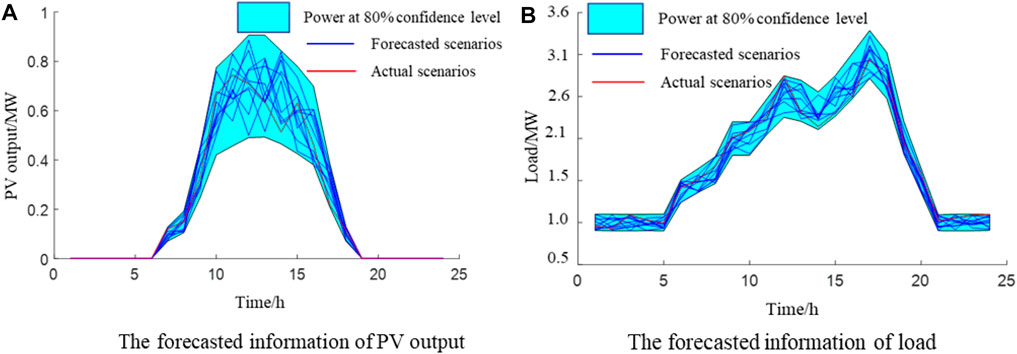
FIGURE 3. Typical scenario for photovoltaic (PV) output and load.

The probability prediction method presented in this paper further considers the time series correlation, which showed better performance in load and PV output prediction. Therefore, to discuss the effectiveness of the prediction method that considers a time series correlation, control experiments were carried out in this section. Another 1,000 sets of typical daily load and PV output forecasted scenarios without considering time series correlation were generated. The performance of the two forecasting methods can be calculated by comparing the obtained results with the actual values. The performance metrics of the two prediction methods are listed in Table 1. The performance metrics of the proposed forecasting method were 4.1e−2 for variance, 2.778% for kurtosis, and 0.456 for skewness. However, the performance metrics for the comparison method were 3e−3, 1.454%, and 0.242, respectively. It can be learned that the proposed prediction method, which takes into account the time series correlation, can forecast the load data more precisely.

TABLE 1

TABLE 1. Load prediction results of the different prediction methods

Analysis of the Energy Management Strategy

Hourly Energy Management Strategy

With the predicted daily load and PV output as inputs, the optimal operation results for the hourly operation model can be calculated and are shown in Figure 4. The ESS keeps charging from 1:00 a.m. to 8:00 a.m. There are two reasons for this phenomenon: 1) the smaller fluctuations of the load and PV and 2) the charging prices were lower. Next, the operation strategies from 10:00 am to 2:00 p.m. are discussed. The energy state of the ESS can fully reflect its charging and discharging behaviors. Therefore, in this paper, the energy state of ESS was selected to present the ESS operation plan. Figure 4 shows the results of the predicted operation plans and the actual ones from 9:00 a.m. to 1:00 p.m. Particularly, the operation plan for the previous moment will be overwritten by the latter moment. For example, the operation plan at 1:00 p.m. covers these plans at times 9:00 a.m.–12:00 p.m. The ESS keeps discharging with an amount of 0.3 MW from 9:00 a.m. to 10:00 a.m. The predicted data are updated at 10:00 a.m., and the newly obtained operation strategy from 10:00 a.m. to 11:00 a.m. orders the ESS to work at the idle status. The operation strategy obtained at 9:00 a.m. and 10:00 a.m. is consistent for 10:00–11:00 a.m. However, with the forecasting information updated, the operation strategy optimized at 10:00 a.m. is modified compared with that at 9:00 a.m. Besides, all the operational strategies for 2:00–5:00 p.m. calculated with the forecasted information from 9:00 a.m. to 11:00 a.m. are charging. This is because the electricity price is relatively low during this period and ESS can store electricity for peak hour usage to reduce the electricity expense.

FIGURE 4

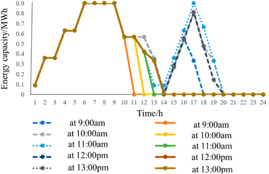
FIGURE 4. Real operation strategies (with line and dot) and predicted strategies (with dash and dot) for energy storage from 9:00 a.m. to 1:00 p.m.

Minute-Level Energy Management Strategy

Furthermore, it can also be learned that the deviation of the energy storage capacity did not exceed 10% of its rated capacity. Hence, in this paper, the given maximum deviation ratio value was set as 10%. This value can be used to guide the degree of matching for the minute-level operation; the time window length for an MPC-based model is an important parameter. In this section, the step size is set as 5 min and three different lengths for the time window are discussed. The time window lengths for three different cases were 3, 6, and 24 h. The minute-level operation results of energy storage for the three different models are presented in Figure 5. The operation results, which set 24 h as the time window length, are the global optimal solution. Compared with the 24-h look-ahead model, the 6-h look-ahead model also contained two charging/discharging cycles, while the 3-h look-ahead model had three charging/discharging cycles. It can be concluded that the model with a 6-h look-ahead is closer to the global operation solution. Thus, in this paper, setting 6 h as the time window length of the look-ahead model is better than that set at 3 h.

FIGURE 5

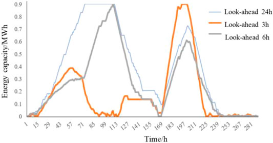
FIGURE 5. Minute-level operation results of the energy storage system for three different models.

We further compared the electrical tariff and objective value in Eq. 20 of the three different hours set and their results are shown in Table 2. The electrical tariff is the first part of Eq. 20. The model with a 24-h look-ahead can obtain the optimal solution. However, in real time, it is difficult to achieve precise prediction of data for 24 h. Hence, it is unrealistic to use the 24-h look-ahead for operation. In this case, with an energy power ratio of 3, the results obtained via the 6-h look-ahead model showed better performance compared with the model set at 3 h.

TABLE 2

TABLE 2. Operating costs and objective for three strategies

Conclusion

In this paper, a two-stage energy management strategy based on stochastic MPC was proposed. The non-parametric probabilistic prediction method embedded in time series correlation was used to generate scenarios of demand and PV output. A two-stage model, which incorporated an hourly operation model and a minute-level one, was presented to refine the energy management of energy storage. From the numerical results, we can conclude that:

1) The proposed probabilistic prediction method embedded in time series correlation has better performance in forecasting the demand and PV output.

2) The deviation ratio of the capacity of ESSs at the terminal point between the hour-level and minute-level operations can be set as 10%.

3) When the energy power ratio is 3, the model looking ahead 6 h has better performance in both run time and solution compared with the model looking ahead 3 h.

Data Availability Statement

The original contributions presented in the study are included in the article/Supplementary Material. Further inquiries can be directed to the corresponding author.

Author Contributions

ZT, JZ, and HZ conceptualized the study. ZT and HZ performed the methodology. ZT and HZ were responsible for software. ZT and JZ validated the results. ZT prepared the original draft. HZ, JZ, and ZT reviewed and edited the manuscript. ZT supervised the study. All authors have read and agreed to the published version of the manuscript.

Funding

This research is supported in part by the Sichuan Science and Technology Program (no. 2021YFG0215 and no. 2021YFSY0052).

Conflict of Interest

The authors declare that the research was conducted in the absence of any commercial or financial relationships that could be construed as a potential conflict of interest.

Publisher’s Note

All claims expressed in this article are solely those of the authors and do not necessarily represent those of their affiliated organizations, or those of the publisher, the editors, and the reviewers. Any product that may be evaluated in this article, or claim that may be made by its manufacturer, is not guaranteed or endorsed by the publisher.

References

Atzeni, I., Ordonez, L. G., Scutari, G., Palomar, D. P., and Fonollosa, J. R. (2013). Demand-Side Management via Distributed Energy Generation and Storage Optimization. IEEE Trans. Smart Grid 4, 866–876. doi:10.1109/TSG.2012.2206060

CrossRef Full Text | Google Scholar

Bakeer, A., Salama, H. S., and Vokony, I. (2021). Integration of PV System with SMES Based on Model Predictive Control for Utility Grid Reliability Improvement. Prot. Control. Mod. Power Syst. 6, 14. doi:10.1186/s41601-021-00191-1

CrossRef Full Text | Google Scholar

Barchi, G., Miori, G., Moser, D., and Papantoniou, S. (2018). “A Small-Scale Prototype for the Optimization of PV Generation and Battery Storage through the Use of a Building Energy Management System,” in 2018 IEEE International Conference on Environment and Electrical Engineering and 2018 IEEE Industrial and Commercial Power Systems Europe (EEEIC/I CPS Europe), Palermo, Italy, June 12–15, 2018 (IEEE), 1–5. doi:10.1109/EEEIC.2018.8494012

CrossRef Full Text | Google Scholar

Dumas, J., Cointe, C., Fettweis, X., and Cornelusse, B. (2021). “Deep Learning-Based Multi-Output Quantile Forecasting of PV Generation,” in 2021 IEEE Madrid PowerTech, Madrid, Spain, June 28–July 2, 2021 (IEEE), 1–6. doi:10.1109/PowerTech46648.2021.9494976

CrossRef Full Text | Google Scholar

Huang, H., Wang, H., and Peng, J. (2020). “Optimal Prediction Intervals of Wind Power Generation Based on FA-ELM,” in 2020 IEEE Sustainable Power and Energy Conference (iSPEC), Chengdu, China, November 23–25, 2020 (IEEE), 98–103. doi:10.1109/iSPEC50848.2020.9350964

CrossRef Full Text | Google Scholar

Li, Z., Wu, L., Xu, Y., Moazeni, S., and Tang, Z. (2021). Multi-Stage Real-Time Operation of A Multi-Energy Microgrid with Electrical and Thermal Energy Storage Assets: A Data-Driven MPC-ADP Approach. IEEE Trans. Smart Grid 1, 1. doi:10.1109/TSG.2021.3119972

CrossRef Full Text | Google Scholar

Liu, J., Cheng, H., Zeng, P., Yao, L., Shang, C., and Tian, Y. (2018). Decentralized Stochastic Optimization Based Planning of Integrated Transmission and Distribution Networks with Distributed Generation Penetration. Appl. Energ. 220, 800–813. doi:10.1016/j.apenergy.2018.03.016

CrossRef Full Text | Google Scholar

Liu, J., Zeng, P. P., Xing, H., Li, Y., and Wu, Q. (2020). Hierarchical Duality-Based Planning of Transmission Networks Coordinating Active Distribution Network Operation. Energy 213, 118488. doi:10.1016/j.energy.2020.118488

CrossRef Full Text | Google Scholar

Małkowski, P., Niedbalski, Z., and Sojka, W. (2021). The Assessment of the Optimal Time Window for Prediction of Seismic hazard for Longwall Coal Mining: the Case Study. Acta Geophys. 69, 691–699. doi:10.1007/s11600-021-00541-5

CrossRef Full Text | Google Scholar

Muller, N., Kouro, S., Zanchetta, P., and Wheeler, P. (2018). “Bidirectional Partial Power Converter Interface for Energy Storage Systems to Provide Peak Shaving in Grid-Tied PV Plants,” in 2018 IEEE International Conference on Industrial Technology (ICIT), Lyon, France, February 20–22, 2018 (IEEE), 892–897. doi:10.1109/ICIT.2018.8352296

CrossRef Full Text | Google Scholar

Nunna, K. H. S. V. S., and Doolla, S. (2014). Responsive End-User-Based Demand Side Management in Multimicrogrid Environment. IEEE Trans. Ind. Inf. 10, 1262–1272. doi:10.1109/TII.2014.2307761

CrossRef Full Text | Google Scholar

Reddy, S. S., Bijwe, P. R., and Abhyankar, A. R. (2015). Joint Energy and Spinning Reserve Market Clearing Incorporating Wind Power and Load Forecast Uncertainties. IEEE Syst. J. 9, 152–164. doi:10.1109/JSYST.2013.2272236

CrossRef Full Text | Google Scholar

Shangguan, Q., Fu, T., Wang, J., Luo, T., and Fang, S. e. (2021). An Integrated Methodology for Real-Time Driving Risk Status Prediction Using Naturalistic Driving Data. Accid. Anal. Prev. 156, 106122. doi:10.1016/j.aap.2021.106122

PubMed Abstract | CrossRef Full Text | Google Scholar

Sharma, S., Verma, A., Xu, Y., and Panigrahi, B. K. (2021). Robustly Coordinated Bi-level Energy Management of a Multi-Energy Building under Multiple Uncertainties. IEEE Trans. Sustain. Energ. 12, 3–13. doi:10.1109/TSTE.2019.2962826

CrossRef Full Text | Google Scholar

Sheikhi, A., Rayati, M., Bahrami, S., and Mohammad Ranjbar, A. (2015). Integrated Demand Side Management Game in Smart Energy Hubs. IEEE Trans. Smart Grid 6, 675–683. doi:10.1109/TSG.2014.2377020

CrossRef Full Text | Google Scholar

Spiliopoulos, N., Wade, N., Giaouris, D., Taylor, P., and Rajarathnam, U. (2017). “Benefits of Lithium-Ion Batteries for Domestic Users under TOU Tariffs,” in 2017 52nd International Universities Power Engineering Conference (UPEC), Heraklion, Greece, August 28–31, 2017 (IEEE), 1–6. doi:10.1109/UPEC.2017.8231966

CrossRef Full Text | Google Scholar

Tang, Z., Liu, J., Liu, Y., Huang, Y., and Jawad, S. (2019). Risk Awareness Enabled Sizing Approach for Hybrid Energy Storage System in Distribution Network. IET Generation, Transm. Distribution 13, 3814–3822. doi:10.1049/iet-gtd.2018.6949

CrossRef Full Text | Google Scholar

Tang, Z., Liu, J., Liu, Y., and Xu, L. (2020). Stochastic reserve Scheduling of Energy Storage System in Energy and reserve Markets. Int. J. Electr. Power Energ. Syst. 123, 106279. doi:10.1016/j.ijepes.2020.106279

CrossRef Full Text | Google Scholar

Tang, Z., Liu, Y., Wu, L., Liu, J., and Gao, H. (2021). Reserve Model of Energy Storage in Day-Ahead Joint Energy and Reserve Markets: A Stochastic UC Solution. IEEE Trans. Smart Grid 12, 372–382. doi:10.1109/TSG.2020.3009114

CrossRef Full Text | Google Scholar

Wan, C., Wang, J., Lin, J., Song, Y., and Dong, Z. Y. (2018). Nonparametric Prediction Intervals of Wind Power via Linear Programming. IEEE Trans. Power Syst. 33, 1074–1076. doi:10.1109/TPWRS.2017.2716658

CrossRef Full Text | Google Scholar

Wan, C., Zhao, C., and Song, Y. (2020). Chance Constrained Extreme Learning Machine for Nonparametric Prediction Intervals of Wind Power Generation. IEEE Trans. Power Syst. 35, 3869–3884. doi:10.1109/TPWRS.2020.2986282

CrossRef Full Text | Google Scholar

Wang, J., Zhong, H., Xia, Q., Kang, C., and Du, E. (2017). Optimal Joint‐dispatch of Energy and reserve for CCHP‐based Microgrids. IET Generation, Transm. Distribution 11, 785–794. doi:10.1049/iet-gtd.2016.0656

CrossRef Full Text | Google Scholar

Xu, J., Chen, Z., Hao, T., Zhu, S., Tang, Y., and Liu, H. (2018). “Optimal Intraday Rolling Operation Strategy of Integrated Energy System with Multi-Storage,” in 2018 2nd IEEE Conference on Energy Internet and Energy System Integration (EI2), Beijing, China, October 20–22, 2018 (IEEE), 1–5. doi:10.1109/EI2.2018.8581926

CrossRef Full Text | Google Scholar

Yin, W., Liu, H., Ni, X., Zhou, H., and Hou, Y. (2018). “A Two-Stage Rolling Scheduling Strategy for Battery Energy Storage in Multi-Periods Electricity Market,” in 2018 IEEE Power Energy Society General Meeting (PESGM), Portland, OR, August 5–10, 2018 (IEEE), 1–5. doi:10.1109/PESGM.2018.8586254

CrossRef Full Text | Google Scholar

Zhou, B., Ma, X., Luo, Y., and Yang, D. (2019). Wind Power Prediction Based on LSTM Networks and Nonparametric Kernel Density Estimation. IEEE Access 7, 165279–165292. doi:10.1109/ACCESS.2019.2952555

CrossRef Full Text | Google Scholar